A Genetic Algorithm-Based Feature Selection
Babatunde Oluleye
eAgriculture Research Group, School of Computer and Security Science, Edith Cowan University, Mt Lawley, Perth, WA, 6050,
Western Australia, Australia Email: [email protected]
Armstrong Leisa
eAgriculture Research Group, School of Computer and Security Science, Edith Cowan University, Mt Lawley, Perth, WA, 6050,
Western Australia, Australia
Jinsong Leng
eAgriculture Research Group, School of Computer and Security Science, Edith Cowan University, Mt Lawley, Perth, WA, 6050,
Western Australia, Australia
Diepeveen Dean
Department of Agriculture and Food,South Perth, 6067, WA, Australia
Abstract – This article details the exploration and application of Genetic Algorithm (GA) for feature selection. Particularly a binary GA was used for dimensionality reduction to enhance the performance of the concerned classifiers. In this work, hundred (100) features were extracted from set of images found in the Flavia dataset (a publicly available dataset). The extracted features are Zernike Moments (ZM), Fourier Descriptors (FD), Lengendre Moments (LM), Hu 7 Moments (Hu7M), Texture Properties (TP) and Geometrical Properties (GP). The main contributions of this article are (1) detailed documentation of the GA Toolbox in MATLAB and (2) the development of a GA-based feature selector using a novel fitness function (kNN-based classification error) which enabled the GA to obtain a combinatorial set of feature giving rise to optimal accuracy. The results obtained were compared with various feature selectors from WEKA software and obtained better results in many ways than WEKA feature selectors in terms of classification accuracy.
Keywords–Feature Extraction, Binary Genetic Algorithm, Feature Selection, Pattern Classification.
I. I
NTRODUCTIONHigh dimensional feature set can negatively affect the performance of pattern or image recognition systems. In other words, too many features sometimes reduce the classification accuracy of the recognition system since some of the features may be redundant and non-informative [1]. Different combinatorial set of features should be obtained in order to keep the best combination to achieve optimal accuracy. In machine learning and statistics, feature selection, which is also called variable selection, attribute selection or variable subset selection, is the process of obtaining a subset of relevant features (probably optimal) for use in machine model construction. There are lots of techniques available for obtaining such subsets. Some of these techniques include Principal Component Analysis (PCA), Particle Swarm Optimization (PSO), Genetic Algorithm (GA) ([9], [10], [11]). More often, lots of researchers in recent times have employed WEKA (Weka (Waikato Environment for Knowledge Analysis) software for dimensionality reduction. However, WEKA software is static in its feature selection approach as the users cannot change the configuration of the concerned feature selectors [25]. GA has been known to be a very adaptive and efficient method of feature selection as reported by ([18],[19],[20]) since the users or
writers can change the functional configuration of GA to further improve their results. As such, a GA-based feature selection (a subspace or manifold projection technique) will be used to reduce the number of features needed by the WEKA Classifiers used in this work. We employed MATLAB GA Toolbox and provided detailed walk-through of its operation. A Feature Subset Selection (FSS) is an operator Fs or a map from an m-dimensional eature space (input space) to n-dimensional feature space (output) given in mapping
rxn rxm
R R
Fs: (1)
where mn and m,nZ, Rrxm is any database or matrix containing the original feature set having r instances or observation,
R
rxn is the reduced feature set containing r observations in the subset selection. This is further illustrated in Figure 1. It is to be noted that Feature selection is inherently a multi-objective problem with two main objectives of minimizing both the number of features and classification error.Fig.1. Illustrative diagram on feature selection
II. C
OMPLETED
ATASETA. Features Generated from the Flavia Dataset
(Dataset1)
The complete dataset for this work comprises of Zernike Moment (ZM), FDs, Lengendre Moments (LM), Hu 7 Moments (Hu7M), Texture Properties (TP) and Geometrical properties (GP) ([22], [23], [24]).The variablesFi,i=1(1)100 , in Table 1 and Table 2 represent the features needed for this work. Thus the feature space of this work is a rxm
R matrix, where r, (number of observations) = 1907 and m, (number of attributes or futures required)= 100.
B. Ionosphere dataset (Dataset2
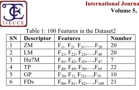
)Copyright © 2014 IJECCE, All right reserved Table 1: 100 Features in the Dataset2
SN Descriptor Features Number
1 ZM F1, F2, F3,...…F20 20
2 LM F21, F22, F23,…,F40 20
3 Hu7M F41, F42, F43,…,F47 7
4 TP F48, F49, F50,…,F69 22
5 GP F70, F71,F72,…,F79 10
6 FDs F80, F81, F82,…,F100 21
Table 2: Hundred (100) features derived from the Flavia Dataset ([27])
Observation F1 F2 F3 F4…….F100
Image 1 X1,1 X1,2 X1,3 X1,4……X1,100
Image 2 X1,1 X1,2 X1,3 X1,4……X1,100
Image 3 X1,1 X1,2 X1,3 X1,4……X1,100
Image 4 X1,1 X1,2 X1,3 X1,4……X1,100
…. ……….
…. ……….
…. ……….
Image 1907 X1907,1 X1907,2 X1907,3…X1907,100
C. Problem Statement
Based on the dataset described in Table 2 the following optimization problem was solved.
Problem:
Given thatnZ, 1n100 and R0100 where:
(i) n = number of features in the reduced feature set. (ii) = Classification error.
Find a subset of features i
F in Table 2 such that the
objective and n are minimized.
III. G
ENETICA
LGORITHM(GA)
Genetic Algorithms (GA) is an optimization technique, a population-based and algorithmic search heuristic methods that mimic natural evolution process of man ([2], [3],[19], [20], [21], [26]). The operations in a GA are iterative procedures manipulating one population of chromosomes (solution candidates) to produce a new population through genetic functionals such as crossover and mutation (in a similar way to Charles Darwin evolution principle of reproduction, genetic recombination, and the survival of the fittest). As documented in [4], the terminology between human genetic and GA can be summarised as shown in Table 3.
Table 3: Comparative Terminology between human genetic and GA
SN Human Genetic GA Terminology 1 chromosomes bit strings
2 genes Features
3 allele feature value
4 locus bit position
5 genotype encoded string
6 phenotype decoded genotype
The fitnesses of the solution candidates (chromosomes) are evaluated using a function commonly referred to as objective or fitness function. In other words, the fitness function (objective function) gives numerical values which are used in ranking the given chromosomes in the population. The formulation of the fitness function depends on the problem being solved. A good example to illustrate a fitness function is the parabola h(x): x→ax2+ bx + c which is used in optimising quadratic functions over admissible real or complex range of values. The symbols {a, b, c} in this expression are constants. The GA in the MATLAB Toolbox is tailored to be a minimiser of objective function as opposed to many other commercially available GA which maximizes. However the maximization problem can be seen as dual form of a minimization problem depending on the user-defined fitness function. To illustrate this, suppose the function h(x) = x2is to be minimized viz min [h(x)], then the dual formulation of this problem is to maximize the negative of h(x), written as max[-h(x)]. Thus maximizing the negative of a function is equivalent to minimizing its positive. In relation to this article, maximizing classification accuracy is equivalent to minimizing the classification error rate.
IV. GA-B
ASEDF
EATURES
ELECTIONA. Generation of Initial Population
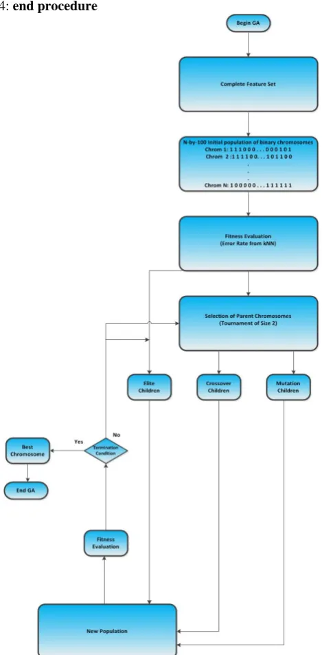
The initial population for this work is a matrix of dimension Population Size x Chromosome Length containing only random binary digits. The Population Size is the number of chromosomes (individuals) in the population, while Chromosome Length (Genome Length) is the number of bits (genes) in each chromosome. It is a good idea to make the population size to be at least the value of the chromosome length so that the chromosomes in each population span the search space [5]. The pseudocode (same as [26]) for initial population is given in Algorithm 1.
Algorithm 1.
Creation of Initial Population (see [26]) 1: procedure POPFUNCTION()2: pop
Binary Matrix of size PopulationSize * GenomeLength 3: Return pop4: end procedure
Fig.2. GA-Based feature Selection (modified from [26])
Table 4: parameters used in GA
GA Parameter Value
Population size 100
Genomelength 100
Population type Bitstrings
Fitness Function kNN-Based Classification Error Number of generations 300
Crossover Arithmetic Crossover Crossover Probability 0.8
Mutation Uniform Mutation
Mutation Probability 0.1
Selection scheme Tournament of size 2
EliteCount 2
B. Fitness Evaluation
For GA to select a subset of features, a fitness function (a driver for the GA) must be defined to evaluate the discriminative capability of each subset of features. The fitness of each chromosome in the population are evaluated using kNN-based fitness function (see Algorithm 1). The Dataset1 is shown in Table 2 comprising of 100 features. The second dataset (Dataset2) contains 34 features. The kNN algorithm solves classification problem by looking for the shortest distance between the test data and training sets in the feature space. Suppose the training set, using Dataset1 and Dataset2,is defined as
} ,..., , ,
{x1 x2 x3 xM
x (2)
where M {1907,34} for the Dataset1 and Ionosphere Dataset (Dataset2) respectively. The M is the number of observations in these dataset. Each xi,i=1(1)100 is a vector containing 100 features as shown in Table 2. The kNN algorithm computes Euclidean distance between test data xtest and the training sets and then find the nearest point (shortest distance) from the training set to the test set. This distance is expressed in Equation 3.
M
m
i test i
test x x x x
D
1
2
) (
) ,
( (3)
The kNN count each categorymin the class information (accumulated as count(xm) using 3 Nearest Neighbors and then report classification results and errors based on the expression:
)) ( max(
arg count xm (4)
subject to:
M
i
m class x
count 1
)
( (5)
Copyright © 2014 IJECCE, All right reserved next generation or mating pool. The iterations involved in
running the GA ensures that the GA reduce the error rate and picks the individual with the least (best) fitness value since error rate is reported for each chromosomes involved and the smallest of error rate is finally picked up by the GA.
ff N
N
fit
exp
1 (6)
= kNN-Based classification error.f
N
= Cardinality of the selected features.The algebraic structure of this equation ensures the learning of the GA, error minimization and reduced number of features selected.
Algorithm 2.
Fitness Function Evaluation ( see [26]) 1: procedure fit()2: FeatIndex Indices of ones from BinaryChromosome 3: NewDataSet DataSet indexed by FeatIndex
4: NumFeat Number of elements in FeatIndex 5: 3 NumNeighborskNN
6: kNNError ClassifierKNN(DataSet,ClassInformation ,NumNeighborskNN) 7: Return kNNError
8: end procedure
C. Generation of children for new population
After fitness evaluation, new population is created using Elitism and Genetic Operators (Crossover and Mutation). In this GA (MATLAB GA Toolbox), three types of children are created to form the new population [5]. They are:
(a) Elite children:
These children are given pushed automatically into the next generation (being those with the best fitness values). Elitism in the GA Toolbox is specified by the identifier "EliteCount" with default value of 2. It is obviously bounded by the population size. This implies "EliteCount"
PopulationSize. With size 2, GA picks the top two best chromosomes and push them automatically to the next generation.(b) Crossover Children:
This is explained in section D below.(c) Mutation Children:
This is explained in section D below.D. Proportion of Elite, Crossover, and Mutation
Children in the New Population
Table 4 shows the configuration of the GA in this work. From Table 4, the length of each chromosome for experimental Dataset2 is 100 since we have a total number of 100 features extracted from the Flavia dataset. The maximum number of generation was set to 300 to avoid the GA been trapped in local optimal. To create new population, the GA performs Elitism, Crossover and Mutation in sequential order.
(1) Elite Children:
The number of elitism as shown in Table 4 is 2. Therefore, the top two kids with the lowest fitness values are automatically pushed in the next generation. Thus, Number (Elite kids) = C1 = 2. This means there are 98 (i.e100-C1) individuals in the population apart from elite kids. From the remaining 98 chromosomes, crossover and mutation kids are then produced.(2) Crossover Children:
The proportion/fraction of the next generation, apart from the left over kids, that are produced by crossover is called Crossover fraction. Crossover fraction used in this work is 0.8. If this fraction is set to one, then there is no mutation kids in the GA, otherwise, there will be mutation kids. With the fraction taken as 0.8, then the number of crossover children will be C2 = round (98 *0.8) = 78(3) Mutation Children:
Finally, number of mutation children is: C3 = 100- C1 - C2 = 100-78-2 = 20.This implies C1 + C2 + C3 = 100
E. Selection Mechanism Used: Tournament
The aim of selection mechanism in GA is to make sure the population (solution candidates) is being constantly improved over all fitness values. The selection mechanism helps the GA in discarding bad designs and keeping only the best individuals. There are many selection mechanism in the GA Toolbox, the default of this being stochastic uniform (with default size 4) but Tournament Selection of size 2 was used in this work due to its simplicity, speed and efficiency ([6], [17], [18]). Also, tournament selection enforces higher selection pressures on the GA (resulting in higher rate of convergence) and makes sure the worst individual does not get into the next generation ([4], [9], [10], [11], [12], [13], [14]). In the GA, two functions are needed to perform tournement selection. The first function generates the players (parents) needed in the actual tournament function, while the second function which outputs the winner of the tournament. The fitnesses of the selected chromosomes are ranked and the best of this becomes the winner. In tournament selection of size 2, two chromosomes are selected from the population after the Elite kids are taken out and the best of the two chromosomes,(using fitness ranking), is selected. Tournament selection is performed iteratively until the new population is filled up.
F. Crossover function
The crossover operator in the GA genetically combines two individuals (parents) to form children for the next generation. Two parents chromosomes are needed to carry out crossover operation. The two chromosomes are taken from tournament selection. The GA uses crossover fraction, say, XoverFrac to specify the number of kids produced by the crossover functional after Elite kids are removed from the current population being evaluated.. The variable XoverFrac, as discussed in the preceding section, is bounded by the inequality 0
XoverFrac
1. The value used for XoverFrac in this work is 0.8 and the crossover function chosen is arithmetic type. In this case, XOR operation is performed on the two parent chromosomes since they are binary ([5], [7], [8], [15], [16]). This is illustrated in Equation 7.CrossOverkids (ii) =
p
1
p
2 (7)where
ii is an index that runs from 1 to the number of kids needed for crossover;The XOR operator
works as follows: 1
1 = 01
0 = 1 0
1 = 1 0
0 = 0So for two binary operands (parent chromosomes) viz; p1 = 1 0 0 0 0 0 0 0 0 0 1 0 0 0 0 1 1 1 0 1
p2 = 0 1 1 1 1 0 1 1 1 1 0 0 0 1 1 1 1 0 1 1 CrossOverKid = p1
p2CrossOverKid = 1 1 1 1 1 0 1 1 1 1 1 0 0 1 1 0 0 1 1 0
G. Mutation function
Mutation is a genetic pertubation of individuals in the population. Mutation ensures genetic diversity and searching of broader solution space. We used uniform mutation as our choice. For uniform mutation, the GA generates GenomeLength set of random numbers (RDs) from uniform distribution. The value of each random number is associated with the position of each gene (bit) in the chromosome. The chromosome is scanned from left to right and for each associated bit, the value of each RD is compared with the mutation probability (denoted as
m p )
and if the RD at position i is less than pm, then gene (bit) at position i is flipped. Otherwise, the gene is left unflipped. This is repeated from the Least Significant Bit (LSB) to the Most Significant Bit (MSB) of each chromosome in the mutation children. As an example, given a parent chromosome
p = 1 1 0 1 1 1 0 1 1 0 0 0 1 0 0 1 0 1 1 0;
The number of bits in this p is 20. Therefore, a set of 20 uniform random numbers are generated, say,
RD20 = [0.5159 0.4161 0.5830 0.5138 0.2839 0.3934 0.2659 0.3776 0.9710 0.2595 0.1807 0.2244 0.5224 0.3166 0.4452 0.4138 0.3362 0.4145 0.5863 0.6220] If the mutation probability is
m
p = 0.3, then m p is compared with each vector entry in RD20 and the following binary vector
int mpo
p is obtained.
int mpo
p = 0 0 0 0 1 0 1 0 0 1 1 1 0 0 0 0 0 0 0 0. The positional index of 1s in
int mpo
p are5, 7, 10, 11, 12. Finally, all the genes in p at locus 5, 7, 10, 11, 12 are flipped, which will then produce a mutation kid as: MutKid = 1 1 0 1 0 1 1 1 1 1 1 0 1 0 0 1 0 1 1 0.
H. New Population (Member of next generation)
The GA keeps evolving until the new population is filled up. The new population is filled by adding individuals from Elite kids, crossover kids, and mutation kids. This is illustrated by Equation 8
NewGeneration = Number(Elitkids) +
Number (Crossover kids) + Number (Mutation kids) (8) This is then evaluated again and the selection-reproduction steps are repeated until the stopping condition is met.
NewGenerationScore = Fitness (NewGeneration) (9)
I. Repeat Until GA termination conditions occur
Once the GA reaches optimum solution, it stops. The code condition at which the GA stops is called stopping
conditions. The two stopping conditions applicable to this work are:
(a) Maximum Number of Generations (Generations
Z+).(b) Stall Generation Limit (StallGenLimit
Z+).The GA can terminate prematurely if the ’Generations’ is not properly set. The value of 'Generations' for this work was set to be 300 while the value 100 was used for StallGenLimit. The GA terminates if the average change in the fitness values among the chromosomes over StallGenLimit generations is less than or equal to Tolfun which is valued as 0.000001. Specifically, the GA examines the difference in values of fitnessess of all generations and if the average of these differences for 100 generations is less than or equal to 0.000001, the GA terminates. This implies genetic homogeneity (similarity in fitness values) among the chromsomes of the generation containing the best chromosome and consequently, the convergence of the GA.
V. S
IMULATION ANDE
XPERIMENTALR
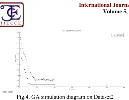
ESULTSBased on the GA configuration in Table 4, the following results were obtained. The carefully chosen fitness function enabled the GA to minimize classification error from kNN. As a proof (from MATLAB documentation [5]), the best fitness and mean fitness should be close in value as the GA reaches the termination condition. The stall generation is number of generations produced by the GA since the last upgrade of the fitness value. The GA terminates at generation 101. This is also evidenced by the GA simulation diagrams in Figures (4 and 5) where the value of the fitness function remains constant from generation 58 to 101 and generation 38 to 101 for the Dataset1 and Dataset2 respectively. The features selected by the GA from both datasets are:
(a) Selected Feature 1 (Dataset1) =1, 6, 12, 15, 18, 56, 64, 71, 72, 75, 78i.e (11% of the original dataset).
(b) Selected Feature 2 (Dataset2) = 2, 3, 5, 7, 8, 34 i.e (17.65% of the original dataset).
The best and mean fitness value, using the kNN classification error for Dataset1 were 0.1746 and 0.181 while that of Dataset2 were 0.06268 and 0.07151. These results are validated in section below.
Copyright © 2014 IJECCE, All right reserved Fig.4. GA simulation diagram on Dataset2
VI. V
ALIDATION OFE
XPERIMENTALR
ESULTSTo validate the GA-FS in this work, the resuts of the GA-based features were compared with a number of WEKA-Based features and test were also made using the selected features on a number of WEKA classifers such as Multi-Layer Perceptron (MLP), Random Forest (RF), J48, Naive Bayes (NB), and classification using regression (RC). The two WEKA feature evaluators used are WEKA Correlation Feature Selection Subset Evaluator (WEKA CFS-SE) and WEKA ranker (Information Gain). The GA was evaluated using fitness function as shown in Equations (4.5). The simulation diagram (Figures 4 and 5) based on the chosen fitness function shows convergence of the GA. The feature indexed by 6 in the Dataset1 cuts across all the selectors. This proves a point that this feature will be useful for building image-based classification systems . This feature is Zernike Moment of order 6 and iteration 0 (i.e ZMI(6,0)). When the Dataset1 was fed into WEKA CFS which is a wrapper-based feature selector, 20 features were reported and this includes the feature indexed by 6 also. Interestingly, the GA selected 11 features ([1, 6, 12, 15, 18, 56, 64, 71, 72, 75, 78]) that were also selected by the WEKA ranker and CFS. The features common to both methods are Zernike moments, Hu moments, Texture properties, and Geometric properties. The GA approach has high level of controllability as the parameters in the GA configuration table can still be fine-tuned to obtain better results. Geometric properties of the Flavia dataset index by the vectors [70, 71, 72, 73, 74, 75, 76, 77, 78, 79] were also selected at rate more than any other features. The third features prefentially selected by all the selectors is Hu 7 moments (indexed by vectors [41, 42, 43, 44, 45, 46, 47]).
Table 7: Classification accuracy using GA and WEKA-Based features on first dataset (Dataset1). SN Selector+WEKA Classifier Accuracy
(%)
RMSE
1 GA+MLP 72.88 0.1105
2 GA+RF 72.37 0.1037
3 GA+J48 67.97 0.1300
4 GA+NB 56.72 0.1222
5 GA+RC 69.70 0.1012
6 WEKA(IG)+MLP 73.52 0.1135
7 WEKA(IG)+RF 74.00 0.1065
8 WEKA(IG)+J48 70.84 0.1267
9 WEKA(IG)+NB 61.25 0.1483
10 WEKA(IG)+RC 74.62 0.1092
11 WEKA(CFS SE)+MLP 76.25 0.1084
12 WEKA(CFS SE)+RF 81.48 0.0961
13 WEKA(CFS SE)+J48 73.36 0.1223
14 WEKA(CFS SE)+NB 71.26 0.1268
15 WEKA(CFS SE)+RC 78.81 0.1017
Table 8: Comparison GA-FS with WEKA feature selectors using Dataset1
SN Feature Selector Selected Features 1 GA 1, 6, 12, 15, 18, 56, 64,
71, 72, 75, 78 2 WEKA (Information
Gain Ranking Filter)
70, 77, 74, 73, 8, 50, 51, 66, 2, 9, 71, 48, 21, 61, 60, 62, 31, 79, 72, 6 3 WEKA (CFS Subset
Evaluator)
1, 2, 6, 7, 12, 15, 16, 41, 43, 45, 51, 65, 66, 70, 71, 73, 74, 75 ,76 , 77
Table 9: Comparison GA-FS with WEKA feature selectors using Dataset2.
SN Feature Selector Selected Features
1 GA 2, 3, 5, 7, 8, 34
2 WEKA (Information Gain Ranking Filter)
5, 6, 33, 29, 3, 21, 34, 8, 13, 7, 31, 22
3 WEKA (CFS Subset
Evaluator)
1, 3, 4, 5, 6, 7, 8, 14, 18, 21, 27, 28, 29, 34
Table 10: Classification accuracy using GA and WEKA-Based features on second dataset (Dataset2).
SN Selector+WEKA
Classifier
Accuracy(%) RMSE
1 GA+MLP 93.02 0.2339
2 GA+RF 94.35 0.1045
3 GA+J48 91.70 .2462
4 GA+NB 90.55 0.2989
5 GA+RC 91.89 0.1988
6 WEKA(IG)+MLP 93.73 0.2388
7 WEKA(IG)+RF 92.59 0.2414
8 WEKA(IG)+J48 91.74 0.2780
9 WEKA(IG)+NB 86.32 0.3387
10 WEKA(IG)+RC 89.74 0.2801
11 WEKA(CFS SE)+MLP 92.31 0.2499
12 WEKA(CFS SE)+RF 92.88 0.2427
13 WEKA(CFS SE)+J48 90.60 0.2982
14 WEKA(CFS SE)+NB 92.02 0.2682
15 WEKA(CFS SE)+RC 90.88 0.2666
VII. C
ONCLUSIONtwo approaches are very small. The features selected by both method on the first and second dataset respectively, are shown in Table 5 & 6. In overall, both the GA method and WEKA-CFS which are wrapper-based feature selectors produced better classification accuracy than WEKA ranker (IG) which is filter-based. The main advatange of the method herein lies in the area of controllability as the GA can be fine-tuned to produce better results all the time by changing the fitness functions. Of all the features selected, ZM had the highest frequency followed by geometric features. The approaches in this work is much more promising than those from previous works such as [27] & [28] as more features are extracted from the images used. With the application of GA for dimensionality reduction, more disciminating features were obtained.
A
CKNOWLEDGMENTThis work was supported by Edith Cowan University, Western Australia under the scholarship scheme ECUIPRS (Edith Cowan University International Postgraduate Research Scholarship.
R
EFERENCES[1] Bruzzone L. Persello C. A novel approach to the selection of robust and invariant features for classification of hyperspectral images. Department of Information Engineering and Computer Science, University of Trento, 2010.
[2] Tian J. Hu Q. Ma X. Ha M. An Improved KPCA/GA-SVM Classication Model for Plant Leaf Disease Recognition Journal of Computational Information Systems , 2012, 18, 7737-7745. [3] Melanie M. An Introduction to Genetic Algorithms A Bradford
Book The MIT Press, 1999.
[4] Sivanandam S. N. Deepa S. N. Introduction to Genetic Algorithms Springer-Verlag , Berlin, Heidelberg, 2008 [5] Mathworks T. Statistics Toolbox User’s Guide The MathWorks,
Inc. 3 Apple Hill Drive Natick, MA 01760-2098, 2013. [6] Eiben A. E. Smith J. E. Rozenberg G. (Ed.) Introduction to
Evolutionary Computing Springer-Verlag Berlin Heidelberg, 2010
[7] Marek O. Introduction to Genetic Algorithms Czech Technical University (http://www.obitko.com/tutorials/genetic-algorithms/ about.php), 1998
[8] Siddique N. Adeli H. Computational Intelligence: Synergies of Fuzzy Logic, Neural Networks, and Evolutionary Computing John Wiley and Sons Ltd, The Atrium, Southern Gate, ChiChester, West Sussex, PO19 8SQ, United Kingdom, 2013. [9] Taherdangkoo Mohammad. Paziresh Mahsa. Yazdi Mehran.
Bagheri Mohammad. An efficient algorithm for function optimization: modified stem cells algorithm. Central European Journal of Engineering. 2012; 3 (1): 3650
[10] Fogel David B. Evolutionary Computation: The Fossil Record. New York: IEEE Press. ISBN 0-7803-3481-7; 1998.
[11] Zhang J. Chung H. Lo W. L. Clustering-Based Adaptive Crossover and Mutation Probabilities for Genetic Algorithms. IEEE Transactions on Evolutionary Computation vol.11, no.3, pp. 326335, 2007.
[12] Goldberg D.E. Korb B. Deb K. Messy genetic algorithms: Motivation, analysis, and first results. Complex Systems, 5(3):493530;1989.
[13] Falkenauer Emanuel. Genetic Algorithms and Grouping Problems. Chichester, England: John Wiley & Sons Ltd. ISBN 978-0-471-97150-4; 1997.
[14] Srinivas M. Patnaik L. ”Adaptive probabilities of crossover and mutation in genetic algorithms,” IEEE Transactions on System, Man and Cybernetics, vol.24, no.4, pp.656667, 1994.
[15] Kjellstrom G. On the Efficiency of Gaussian Adaptation. Journal of Optimization Theory and Applications 71 (3): 589597. doi:10.1007/BF00941405; 1991.
[16] Rania Hassan. Babak Cohanim. Olivier de Weck. Gerhard Vente r . A comparison of particle swarm optimization and the genetic algorithm. 2005.
[17] Civicioglu P. Transforming Geocentric Cartesian Coordinates to Geodetic Coordinates by Using Differential Search Algorithm. Computers &Geosciences 46: 2012; 229247. doi:10.1016/ j.cageo.2011.12.011
[18] Baudry Benoit. Franck Fleurey.Jean-Marc Jezequel.Yves Le Traon. Automatic Test Case Optimization: A Bacteriologic Algorithm. IEEE Software (IEEE Computer Society) 22 (2): 2005: 7682. doi:10.1109/MS.2005.30.
[19] Crosby Jack L. Computer Simulation in Genetics. London: John Wiley & Sons. ISBN 0-471-18880-8; 1973.
[20] Akbari Ziarati. A multilevel evolutionary algorithm for optimizing numericalfunctions” IJIEC 2 ; 419430 ; 2011 [21] Holland John. Adaptation in Natural and Artificial Systems.
Cambridge, MA: MIT Press. ISBN 978-0262581110; 1992. [22] Hu M K. Visual Pattern Recognition by Moment Invariants, IRE
Trans. Info. Theory, vol. IT-8, pp.179187, 1962.
[23] Zernike F. Beugungstheorie des Schneidenverfahrens und Seiner Verbesserten Form, der Phasenkontrastmethode. Physica 1 (8): 689704; 1934.
[24] Fourier J. B. Joseph. The Analytical Theory of Heat, The University Press; 1878.
[25] Mark Hall. Eibe Frank. Geoffrey Holmes. Bernhard Pfahringer. Peter Reutemann . Ian H. Witten. The WEKA Data Mining Software: An Update; SIGKDD Explorations, Volume 11, Issue 1; 2009
[26] BABATUNDE Oluleye. ARMSTRONG Leisa. LENG Jinsong. DIEPEVEEN Dean. Zernike Moments and Genetic Algorithm: Tutorial and Application. British Journal of Mathematics and Computer Science. 4(15): 2217-2236.
[27] Wu Stephen Gang. Bao Forrest Sheng. Xu Eric You. Wang Yu-Xuan. Chang Yi-Fan. Xiang Qiao-Liang. A Leaf Recognition Algorithm for plant Classification Using Probabilistic Neural Network. In Signal Processing and Information Technology, 2007 IEEE International Symposium on (pp. 11-16). IEEE; 2007.