Improving Water Level Forecast of an Oceanographic Model in Malacca Strait Based on Data-Driven Open Boundary Correction

Improving water level forecast of an

oceanographic model in Malacca Strait based on

data-driven open boundary correction

Xuan Wang

_{, Serene Hui Xin Tay}

_{, and Vladan Babovic}

[email protected], [email protected], [email protected]

Abstract

Numerical model is an indispensable tool for understanding oceanographic phenomena and resolving associated physical processes. However, model error cannot be avoided due to limitations such as underlying assumption, insufficient information of bathymetry or boundary condition and so on. Data assimilation technique thus becomes an effective and essential tool to improve prediction accuracy. Updating of output is an efficient way to correct the model, but it is often carried out locally at specific locations in the model domain where measurement is available. In this study, instead of correcting output of numerical model locally, we propose to combine local correction and input correction to update open boundary of numerical model. The open boundary condition is corrected through spatial interpolation algorithm based on nearby observation in the hindcast period. Then the local forecast at measured location is distributed using the same interpolation scheme to update the boundary in the forecast period. Such boundary correction not only explores the variation in the future time step from the input updating but also allows the backbone physics embedded in numerical model to resolve the hydrodynamics in the entire computational domain.

1

Introduction

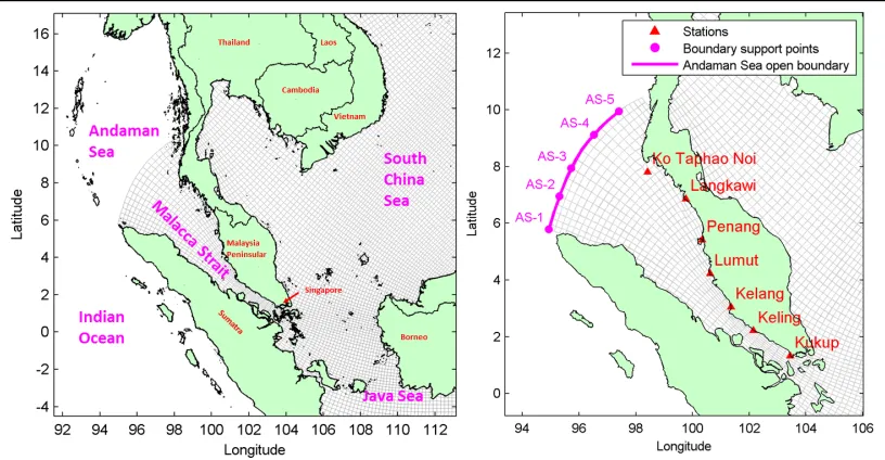
Geographically located between Andaman Sea and South China Sea, water levels in Malacca Strait are indirectly driven by tide and hydrodynamic components from the two oceans: Indian Ocean and Pacific Ocean (Figure 1). Numerical models such as (Kurniawan et al., 2011, 2015, Tay et al., 2013, 2016) have represented tidal and non-tidal flows well in the strait. As the demand of real-time forecasting is getting higher, data assimilation techniques have been attempted in earlier studies to

* _{Created the first draft of this document}

† _{Masterminded EasyChair and created the first stable version of this document} ‡ _{Created the first draft of this document}

Volume 3, 2018, Pages 2301–2309

improve water level forecast from numerical model (Babovic and Keijzer, 2000; Sannasiraj et al., 2004; Babovic, 2009; Wang and Babovic, 2014; Wang, Babovic and Li, 2017). However, due to limited current velocity data, these studies are mainly focusing on water level prediction. Thus the corresponding flow pattern based on this updated water level could not be described using this forecast method. The flow pattern has to be simulated by a physics-based numerical model. Tay et al. (Tay et al., 2016) have shown that superimposing satellite altimetry derived Sea Level Anomalies (SLA) on tidally prescribed open boundary of model have significantly improved the water level representation in Malacca Strait. The simulated hydrodynamic also showed a seasonal volume transport through Malacca Strait and Singapore Strait. However, this approach of modelling is only feasible in the hindcast mode where historical water level observation is already made available. In order to apply the same modelling approach in an operational forecast, this paper proposes to use data assimilation technique to predict the open boundary condition of the numerical model. In this paper, the observed water level located near boundary are first forecasted and then distributed to the open boundary based on the estimation spatial structure. It can utilize the information from both observation and numerical model and thus provide a better driven force to the numerical model to improve its forecasting ability. The objective of this paper is to develop an efficient method to predict the hydrodynamics in Malacca Strait accurately using numerical model with data-driven open boundary correction.

Figure 1 Extent of simulation area, Open boundary, boundary support point and observation station

2

Material and methods

2.1

Data

Hourly observed water level data from University of Hawaii Sea Level Center (UHSLC) (http://uhslc.soest.hawaii.edu/) are used to derive sea level anomalies (SLA) observed in Malacca Strait at seven stations: Ko Taphao Noi, Langkawi, Penang, Lumut, Kelang, Keling and Kukup (Figure 1). SLA are derived by predicting tide using 65 tidal constituents and subtract it from observed water level (Rao and Babovic, 2009).

2.2

Physics-based numerical model

The physics-based numerical model used in this study is built by (Tay et al., 2013) and is set up in Delft3D modelling environment. Figure 2 shows domain extent, open boundaries and bathymetry of model. Spatially varying curvilinear grid (total 12335 grid cells) of the model is schematized in a way whereby the areas close to the open boundaries are of lower resolution of 30 to 50 km while the area of main interest, Singapore and Malacca Straits, are of higher resolution of 5 to 10 km.

Open boundary tidal forcing is prescribed as water level variations by means of amplitudes and phases of the eight main tidal constituents; O1, K1, M2, S2, Q1, P1, N2 and K2. Bathymetry data is based on ETOPO1 dataset (Amante and Eakins, 2009) and bathymetry of other numerical models covering the same domain such as (Gerritsen, Schrama and van den Boogaard, 2003; Kurniawan et al., 2011). Bed roughness represented by Manning friction coefficient spatially varies from 0.015 to 0.400 m1/3_{/s over the model domain. Time step of model is 5 minutes, and it takes about 1.3 hour} computational time for 1 year simulation on an Intel Core i7-2600 (quad core) 3.4 GHz CPU PC. Details of tidal calibration and representation of model is described by (Tay et al., 2013). 6-hourly 0.75 degree horizontal resolution surface wind and pressure fields obtained from ECMWF ERA-Interim database (www.ecmwf.int) are applied to the model to generate non-tidal barotropic flow in the model domain (Kurniawan et al., 2015; Tay et al., 2016).

Figure 2 Domain extent, bathymetry and open boundaries of the physics-based numerical model

2.3

Modified Local Model

The MLM proposed by (Wang, Babovic and Li, 2017) is applied to predict SLA at station Ko Taphao Noi, Langkawi and Penang with long time forecasting accuracy. These three stations are chosen because they are located closest to the Andaman Sea open boundary where the tilt is to be imposed. Three forecast horizons (1 day, 5 days and 10 days) are selected in this study. The MLM updated from Local Model (LM) predicts the time series 𝑥"_#by involving the chaos theory. Given a chaotic time series correlated with 𝑥"#, 𝑥"# can be estimated through some correlated non-linear

function from , i.e.

(1) Based on Taken’s embedding theory (Takens, 1981), given a time series e.g. at reference time

point , a proper embedding , could be created to present

underlying order of corresponding dynamic system to predict the scalar value of this time series in the future, i.e.

(2) So

tn

y

tn

y

)

(

n t

t

g

y

x

=

tn

y

n

t ( )

{

}

n n n e

n t t t d

Y t = y y -t y - - t

ˆ ( )

n

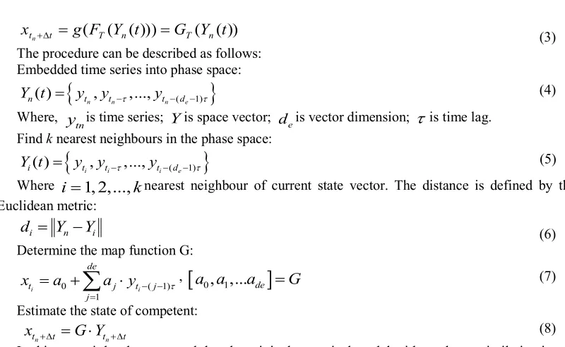
(3) The procedure can be described as follows:

Embedded time series into phase space:

(4)

Where, is time series; is space vector; is vector dimension; is time lag. Find k nearest neighbours in the phase space:

(5) Where nearest neighbour of current state vector. The distance is defined by the Euclidean metric:

(6)

Determine the map function G:

, (7)

Estimate the state of competent:

(8)

In this paper it has been proved that the original numerical model without data assimilation is still able to capture the hydrodynamic movement. It can be believed that the water level from model simulation is correlated to their observation value. Therefore, 𝑥"# is the measured SLA at three

observed location and is water level from numerical model. The three optimal embedding parameters , , are determined by Genetic Algorithm (Goldberg, 1989). In this paper, the parameters for the three observed stations are tabulated in Table 1.

Stations

Ko Taphao Noi 15 4 1

Langkawi 23 2 1

Penang 20 4 1

Table 1 Optimal embedding parameters at forecasted locations

2.4

Approximated Ordinary Kriging

The predicted SLA using MLM at the three stations are then distributed using Approximate Ordinary Kriging (AOK) method (Wang and Babovic, 2014) to the Andaman Sea open boundary to estimate the SLA (or tilt) at boundary points AS-1, AS-2, AS-3, AS-4 and AS-5 (Figure 1). The AOK derived from Ordinary Kriging (OK) is one technique for spatial interpolation. It expresses the spatial dependence structure through an approximate variogram. The fundamental difference between AOK and other Kriging methods is to it approximates the variogram of variable of interest with variogram of another variable having similar spatial characteristics. For instance, given observations of variable at different stations, the variogram derived from should be able to capture the underlying spatial relationship of these stations. If there is another variable having similar spatial characteristics, the variogram derived from ( ) should reflect a spatial relationship similar to . Thereby, this derived variogram can be used as the approximated variogram to calculate the weight function of . It has been clarified in previous section that the numerical model can reasonable simulate the hydrodynamic condition, so it is assumed that the numerical simulated water level can

)) ( ( ))) ( (

(F Y t G Y t

g

xtn+Dt = T n = T n

{

}

( ) , ,...,

n n n e

n t t t d

Y t = y y -t y - - t

tn

y Y d_e

t

{

}

( ) , ,...,

i i i e

i t t t d

Y t = y y _-t y _{- - t}

1, 2,...,

i

=

k

i n i

d = Y -Y

0 ( 1)

1

i i

de

t j t j

j

x a a y _{- - t}

=

= +

å

[

]

n n

t t t t

x _+D =G Y× _+D

tn

y

t

e

d

t

x

_g

_x

y

y

_g

_x

access the similar spatial dynamics of the actual water level spatial structure. The proposed AOK scheme is executed in several steps as follows.

Calculate the approximated variogram

By assuming the variogram is only dependent on the length of spatial lag (also called distance lag), it can be calculated from Equation (4) (Bogaert, 1996):

(9)

where, is the approximated variogram of SLA (its subscript indicates points index and the superscript indicates corresponding variable); and the starting and ending point, respectively;

the distance between starting and ending point; the model simulated water level at point

; the variance of data series .

Since the variable can be obtained at non-measured point , its variograms at this point can also be calculated through Equation (9).

Estimate the weights

The weights are then computed from the Kriging linear equations:

(10)

where, is the approximated variogram between measured point and non-measured point ; the Lagrange multiplier.

Perform optimal interpolation

The variable at target non-measured stations at each time instance can be estimated through Equation (11) based on the nearby measurements.

(11)

Where, is interpolated value at non-measured point at time instance .

3

Results

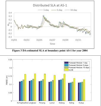
Three forecast horizons 1 day, 5 days and 10 days are selected for the tilt prediction using MLM and AOK as described earlier and the predicted SLA at boundary point AS-1 is shown in Figure 3. The forecasted results from 1-day to 10-day show to be of similar temporal trend, but as the forecast horizon increases, the forecasted results deviate further from the 1-day SLA forecast. The numerical model is simulated with the predicted tilt imposed at the Andaman Sea open boundary. Figure 4 and Figure 5 present the root mean squared error (RMSE) and correlation coefficient of the water level at

mn

g

ˆ

1

ˆ

( )

(

, )

( ( )

( ))

2

mn

h

s

h s

Var y s

y s

g

=

g

=

g

+

=

-g

ˆ

x

m

s

s

h

y s

( )

m

s

Var

y s

( )

-

y s

( )

y

s

g

pm

w

w

ï

ï

î

ïï

í

ì

=

=

=

+

å

å

n pn mn

w

N

m

w

1

)

,...,

1

(

ˆ

ˆ

µ

g

g

mp

g

ˆ

s

s

µ

x

1

ˆ( ,

)

( ,

)

N

p n pm m n

m

x s t

t

w x s t

t

=

+

D

=

å

+

D

ˆ( ,

)

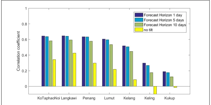
the seven stations in Malacca Strait compared to observation, respectively. Compared to the model result without tilt application, application of predicted tilts at Andaman Sea open boundaries gives significant water level prediction improvement in Malacca Strait with RMSE reduction of up to 0.05 m and correlation improvement of more than 0.5. Among three forecast horizons, the tilt with 1-day horizon gives the best water level prediction. It is noted that the forecast accuracy does not deteriorate significant with increasing forecast horizon as the maximum difference in RMSE between 1-day and 10-day forecast horizons is less than 0.02 m. One reason is due to the forecasted results deviation at open boundary. Another reason could be that the tilt imposed in the numerical model at Andaman Sea open boundary represents water level variation induced by the large-scale ocean circulation in Indian Ocean which is of a longer time scale of weeks or months as compared to tide. It is noted that the correlation of water level prediction in the southern Malacca Strait i.e. Station Kukup and Keling is relatively poor, even after the application of tilt. This is because the hydrodynamics in southern Malacca Strait is highly complex. (Kurniawan et al., 2011, 2015, 2017, Tay et al., 2016, 2017) have pointed out that this area is a major tidal mixing zone between Indian Ocean and South China Sea. (Tay et al., 2016) have also shown that the local non-tidal hydrodynamics are heavily influenced by both Indian Ocean and South China Sea and their degree of influence is seasonally varying.

Figure 3 DA-estimated SLA at boundary point AS-1 for year 2004

Figure 5 Correlation coefficient of water level at seven stations in Malacca Strait

4

Conclusion

This paper has presented an efficient approach of integrating data and physics-based model to improve water level prediction in Malacca Strait. This approach targets at providing an improved open boundary condition and then allows the numerical model to compute the water level by resolving the physics and improves the prediction everywhere in the model domain. The authors believe that this is one of the most physically realistic and efficient data-model integration approaches to predict the hydrodynamics over the entire model domain. In this paper, the SLA is first forecasted using MLM method station Ko Taphao Noi, Langkawi and Penang and spatially distributed based on AOK method to generate the SLA forecast at the numerical open boundary in Andaman Sea known as ‘tilt’. The numerical model is then simulated with its deterministic tidal forcing and the forecasted tilt at the Andaman Sea open boundary with surface forcing of wind and pressure. Three forecast horizons 1, 5 and 10 days are tested in this paper. Results show improvement of up to 5 cm in RMSE and more than 50 percent improvement in correlation. The value of this data and model integration approach is the long time forecast accuracy whereby the reduction of RMSE from a 1-day to a 10-day forecast is less than 2 cm. In conclusion, this data and model integration approach proposed in this paper shows high potential in operational hydrodynamic forecast in Malacca Strait, and possible applications in other parts of the world.

References

Amante, C. and Eakins, B. W. (2009) ‘ETOPO1 1 Arc-Minute Global Relief Model: Procedures, Data Sources and Analysis’, NOAA Technical Memorandum NESDIS NGDC-24, p. 19 pp.

Babovic, V. (2009) ‘Introducing knowledge into learning based on genetic programming’, Journal of Hydroinformatics, 11(3–4), pp. 181–193.

Babovic, V. and Keijzer, M. (2000) ‘Forecasting of river discharges in the presence of chaos and noise’, in Flood issues in contemporary water management. Springer, pp. 405–419.

Bogaert, P. (1996) ‘Comparison of kriging techniques in a space-time context’, Mathematical Geology. Springer, 28(1), pp. 73–86.

the seas of South-East Asia using altimeter data and adjoint modelling’, in XXX IAHR Congress. Thessaloniki, pp. 239–246.

Goldberg, D. E. (1989) Genetic Algorithms in Search, Optimization and Machine Learning. Addison-Wesley Longman Publishing Co., Inc.

Kurniawan, A. et al. (2011) ‘Sensitivity analysis of the tidal representation in Singapore Regional Waters in a data assimilation environment’, Ocean Dynamics, 61(8), pp. 1121–1136. Available at:

http://www.scopus.com/inward/record.url?eid=2-s2.0-81255134078&partnerID=40&md5=2efecd1d86769b6839c6ec20a940c215.

Kurniawan, A. et al. (2015) ‘Analyzing the physics of non-tidal barotropic sea level anomaly events using multi-scale numerical modelling in Singapore regional waters’, Journal of Hydro-Environment Research, 9, pp. 404–419.

Kurniawan, A. et al. (2017) ‘Determining tidal mixing zone using data driven model in Malacca Strait’, in IAHR 2017 World Congress. Kuala Lumpur.

Rao, R. and Babovic, V. (2009) ‘Establishing Sea Level Anomaly patterns using Mutual Information theory’, in 33rd IAHR Congress. Vancouver, Canada.

Sannasiraj, S. A. et al. (2004) ‘Enhancing tidal prediction accuracy in a deterministic model using chaos theory’, Advances in Water Resources, 27(7), pp. 761–772. Available at:

http://www.scopus.com/inward/record.url?eid=2-s2.0-3042563456&partnerID=40&md5=a4dc7aeecd32bc0e5e5ebf74d55ec843.

Takens, F. (1981) ‘Detecting strange attractors in turbulence’, in Rand, D. and Young, L.-S. (eds)

Dynamical Systems and Turbulence, Warwick 1980. Springer Berlin / Heidelberg, pp. 366–381. doi: 10.1007/BFb0091924.

Tay, S. H. X. et al. (2013) ‘Further improvement of tidal representation in the South China Sea and the Southeast Asian waters’, in 2013 IAHR Congress. Chengdu.

Tay, S. H. X. et al. (2016) ‘Sea level anomalies in straits of Malacca and Singapore’, Applied Ocean Research, 58, pp. 104–117. doi: 10.1016/j.apor.2016.04.003.

Tay, S. H. X. et al. (2017) ‘Hydrodynamic modelling of Singapore and Malaccas straits for operational forecast and management’, in IAHR 2017 World Congress. Kuala Lumpur, p. 7.

Wang, X. and Babovic, V. (2014) ‘Enhancing water level prediction through model residual correction based on Chaos theory and Kriging’, International Journal for Numerical Methods in Fluids, 75(1), pp. 42–62. Available at: http://www.scopus.com/inward/record.url?eid=2-s2.0-84897526647&partnerID=40&md5=6c834cec7dec91a0ea4089be4517582a.