Solid Phase Equation of State Application for Wax Formation Prediction in Petroleum Mixtures

23

Solid Phase Equation of State Application for Wax Formation

Prediction in Petroleum Mixtures

S. A. Mousavi Dehghani1∗, M. Vafaie Sefti2, H. Mehdizadeh2 and H. Shirkhanloo1

1- RIPI, West End Entrance Blvd, Olympic Village Blvd, Tehran, Iran.

2- Chemical Engineering Department, Tarbiat Modarres University, Tehran, Iran.

Abstract

Precipitation of solid paraffins is one of the most common problems in the oil industry, imposing high operating costs. There have been a great many efforts for the prediction of solid paraffins precipitation up to now. Most of them were based on activity coefficient models accounting to solid phase non-ideality or the multi-solid model to calculate the number of precipitated solid phases. In this work, solid phase behavior is predicted by a solid equation of state. At first, by using the thermodynamic method (subcoled liquid) for pure solid phase fugacity from pure liquid fugacity, the solid EOS parameters are tuned.

The tuned solid EOS can then be directly applied for the prediction of the amount of precipitated solid paraffins (waxes) in the oil samples. The proposed equations system in this work is solved by a proper mathematical method. The obtained results of wax precipitation in this work are in good agreement with the experimental data.

Keywords: Solid Paraffin, Solid Phase Equation of State, Wax Precipitation, Multi-solid model

∗ Corresponding author: E-mail: [email protected]

Introduction

Wax deposition from gas and oil production facilities and pipelines is undesirable. The flow-lines and process equipment may be plugged by wax deposition. Different physical and chemical methods have been proposed to remove deposited solids, which increase operating costs. A reliable model for wax precipitation calculation is highly valued for the design and operation of flowlines.

Since the 1990s, many efforts have been made to predict conditions under which the

24 Iranian Journal of Chemical Engineering, Vol. 5, No. 2 were proposed based on the activity

coefficient model assuming the non-ideality of liquid and solid phases [3, 4]. Solid phase transition and vapor phase were then considered in other works [5-7]. The non-ideality was defined using Wilson or UNIQUAC equations. Lira-Galeana et al. [8] developed the multi-solid approach in 1996. In this model, it is assumed that the solid wax consists of several pure solid phases, where the number and nature of these phases will be obtained from phase stability analysis. Coutinho showed that the solid phase is a multi-solid solution in nature and this is supported by the experimental data [9]. In this work, the wax-precipitation model based on solid phase equation of state will be presented. The multi-solid approach is used because of its wide acceptability and limitation in using solid phase equation of state. The parameters of the equation of state are obtained in the case that vapor, liquid and solid phases are presented in the system.

Solid Phase Equation of State

There are a few EOS's which can be applied to predict solid, liquid and vapor phase behavior simultaneously [10,11]. One of these EOS types is the TST1 equation of state that is used in this work [11]. The general form of the equation is:

) )(

(v ub v wb a b

v RT P

+ +

− −

= (1)

where, u and w are 3 and -0.5 respectively. Also,

c c

c R T P

a =0.470507 2 2/ (2)

c c

c RT P

b =0.0740740 / (3)

296296 .

0

=

c

Z (4)

1- Twu – Sim - Tassone

c a

a =α (5)

Alpha function for liquid and vapor phases could be used in conventional polynomial form or in exponential form. In this equation, a new alpha function is introduced for the solid phase, which will be discussed later. In order to calculate fugacity of each component in pure solid state, the following equation is used [12].

dP RT

v dT RT

H f

dln =− ∆ ₂ + ∆ (6)

Where f is fugacity, ∆His enthalpy change as result of the change in system temperature, and ∆vis partial molar volume change by pressure.

By integrating the above equation from the triple point pressure to the system pressure for liquid and solid phases and dividing the two equations, the following relation will be obtained. In this equation, ∆Hf and ∆v are supposed to be independent of pressure and temperature.

RT vP T

T RT

H f

f

f f

L

S ∆

−    

  − ∆

−

= 1

ln (7)

Where ∆H f and Tf are melting enthalpy and melting point respectively. These parameters can be calculated as follows:

i i

f

MW MW

T =374.5+0.02617 −2.0172×104/

or

(

)

421 63 1936112 63 7 8945 1 .

f

T = . − . exp − . ( N− )

(8)

Where N and MW_i are carbon number and molecular weight respectively.

f i f

T MW

H =0.1426

∆

or

f i f

T MW H =0.05276

Iranian Journal of Chemical Engineering, Vol. 5, No. 2 25

Other correlation may be used for both parameters [1, 2, 8 16].

At very low pressures (to zero pressures), eq. 7 change to:

      − ∆ −

= f _f

L S T T RT H f f 1 ln (10)

This equation is similar to the equation that was proposed by Prausnitz et al. [13] for the calculation of solid phase fugacity. If the fugacity is calculated at zero pressure,

1 1

1

S

* * S

* S * S

* * S

f

ln ln b ln( v )

P

a v w

ln

( w u ) b v u

  = − − − −        ₊  − ₋ _ _ +   (11) Where, 1 2 2 1 4 2 /

* S * S * S

* S

* * *

a a a

v u w u w uw

b b b

_{     }   _{ }  = _ − − _−_ + − _ − _ + _    _   _    (12) * 2 2 Pa a R T = (13) * Pb b RT = (14)

Where u and w are the parameters of the equation of state. Combining equations 7 to 10 results in:

1

1 1

1

* S *S

* * S

* * S

L f

f

a v w

ln b ln( v ) ln

( w u ) b v u

f H T

ln

P RT T

∆  ₊  − − − − − _ _ − _ + _   _{ } = _ _− _ − _   (15)

The only unknown variable in the above equation is S

a*

. Therefore, the equation is solved to obtaina*Sfor different tempera-tures. The parameters of predefined solid alpha function are calculated by correlating the data to the following equation

) 7 . 0 ( ) 1 ( ) 1 ( 1 )

( 0.5 r

n r S r s S T T m T l

T = + − + − S −

α

(16)

In which αScan be calculated using

/

S S

c

a a

α = (17)

P T R a a S S 2 2 * = (18)

In order to calculate the optimum parameters, the following function was used to minimize the difference between the experimental data and the calculated values from eq. 11.

0 5

2

1 1 1

0 7

s n .

s r ,i s r ,i

s

r ,i i

F ( l ( T ) m ( T )

( . T ) α )

= + − + −

− −

∑

(19)

The simplex-Nelder-Mead algorithm was utilized to obtain the optimum parameters, which minimizes the objecting function. Due to the nonlinearity of the function, the results will drastically depend on the initial guess for the optimal parameters. To avoid this problem, the optimization problem is run for different starting points.

Wax Precipitating Model

The vapor-liquid-solid equilibrium states are defined as follows:

Mass balance for precipitating components:

0 = − + +

∑

i n x n n z n

y

P

26 Iranian Journal of Chemical Engineering, Vol. 5, No. 2 Where,

1,..., _c , 1,..., _P

i = N j = N

NP: Number of precipitated solid phases

NC: Number of components

Mass balance for non-precipitating components:

0

i

v V L L f F

i i

y n +x n −z n =

(21)

Equality of fugacities in the liquid and vapor phases for all components gives:

0

V L

i i

f −f = ₍₂₂₎

And for the liquid and solid phases for precipitating components:

0

i S L i

f −f = ₍₂₃₎

Summation of mole fractions in liquid and gas phases are equal to unity

1

1 0

Nc

i i

x

=

− =

∑

1

1 0

Nc

i i

y

=

− =

∑

All the equations above constitute a system of equations, which can be solved to define the equilibrium system completely. An error function is introduced to check the convergence of the system of equations.

2 2

1

( )

C P

N N

i i

f δ δ

+ +

=

=

∑

Whereδi's are the right hand expressions in

equations 20 to 25.

Results and Discussions

The composition of oil samples and some synthetic mixtures which are used in this research, are given in Tables 1-4.

Table 1. Mole fractions for two synthetic mixtures [7]

Mixture B Mixture C

Component

0.5101 0.5876

n-C10

0.0819 0.0513

n-C18

0.0694 0.0486

n-C19

0.0590 0.0463

n-C20

0.0506 0.0440

n-C21

0.0433 0.0418

n-C22

0.0373 0.0397

n-C23

0.0319 0.0378

n-C24

0.0274 0.0359

n-C25

0.0236 0.0342

n-C26

0.0202 0.0327

n-C27

0.0176 0

n-C28

0.0148 0

n-C29

0.0127 0

n-C30

Table 2. Mole fractions for a synthetic mixture [14]

Bim 13

Component

Bim 13

Component

0.61

C34

80.01

C10

0.53

C35

7.09

C18

0.45

C36

6.09

C19

5.220

Iranian Journal of Chemical Engineering, Vol. 5, No. 2 27

Table 3. Heavy oil fractions analysis [5]

Oil 5

MW Mole percent

Pseudocomponent

167.0 4.4627

P-C10+

160.0 6.4827

N-C10+

160.0 15.126

A-C10+

237.0 2.9096

P-C15+

233.0 3.8627

N-C15+

233.0 8.9664

A-C15+

307.0 1.5426

P-C20+

302.0 2.1514

N-C20+

302.0 5.0199

A-C20+

375.0 0.7856

P-C25+

372.0 1.389

N-C25+

372.0 3.2409

A-C25+

449.0 0.3528

P-C30+

440.0 1.4348

N-C30+

440.0 1.4348

A-C30+

511.0 0.1377

P-C35+

512.0 1.5694

N-C35+

512.0 0.0174

A-C35+

590.0 0.0648

P-C40+

587.0 1.1964

N-C40+

587.0 0.0491

A-C40+

713.0 0.0259

P-C46+

724.0 0.3143

N-CP1+

724.0 1.8285

A-CP1+

901.0 0.2257

N-CP2+

901.0 1.3396

A-CP2+

Table 4. Heavy oil fractions analysis [5]

Oil 6

MW Mole percent

Pseudocomponent

157.0 3.5922

P-CP1

157.0 4.7712

N-CP1

157.0 4.7712

A-CP1

201.0 2.7858

P-CP2

201.0 4.5495

N-CP2

201.0 4.5495

A-CP2

252.0 1.8055

P-CP3

252.0 2.9829

N-CP3

252.0 4.4744

A-CP3

300.0 1.2238

P-CP4

300.0 2.9018

N-CP4

300.0 4.3527

A-CP4

563.0 0.3674

P-CP5

563.0 2.5116

N-CP5

563.0 5.1937

A-CP5

654.0 0.0581

P-CP6

654.0 1.0319

N-CP6

654.0 1.6277

A-CP6

666.0 0.0736

P-CP7

666.0 1.0099

N-CP7

666.0 2.8634

A-CP7

744.0 0.8611

N-CP8

744.0 2.1707

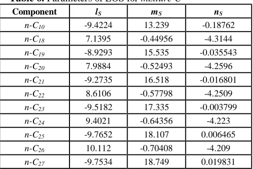
28 Iranian Journal of Chemical Engineering, Vol. 5, No. 2 The parameters of the equation of state (ls,

ms, ns) are evaluated as discussed in the previous section. The optimal values for the mentioned parameters for the oil samples are shown in Tables 5-9. The initial guess for the system of equilibrium equations is given from the results of a two-phase flash calculation. Then, the dogleg method [15] is applied to check the convergence criteria, i.e. the value of the right-hand side expression in equation 19 should be less than 1e-7. If the criterion is not met, the program will shift to simplex

algorithm which uses the results of the previous step as the initial points. There is a normalizing step which filters the incoming physically unacceptable data. The physical properties data can be obtained from the concerned reference data-books and/or they can be estimated from the published correlations for thermodynamic properties. Having two parameters of the true boiling point, molecular weight and specific gravity one can estimate the thermo-physical properties of the components.

Table 5. Parameters of EOS for mixture B

nS

mS

lS Component

-0.18762 13.239

-9.4224

n-C10

-4.3144 -0.44956

7.1395

n-C18

-0.035543 15.535

-8.9293

n-C19

-4.2596 -0.52493

7.9884

n-C20

-0.016801 16.518

-9.2735

n-C21

-4.2509 -0.57798

8.6106

n-C22

-0.0037988 17.335

-9.5182

n-C23

-4.223 -0.64356

9.4021

n-C24

0.006465 18.107

-9.7652

n-C25

-4.209 -0.70408

10.112

n-C26

0.019831 18.749

-9.7534

n-C27

-4.198 -0.76167

10.816

n-C28

0.020441 19.304

-9.9905

n-C29

-4.1968 -0.81451

11.444

n-C30

Table 6. Parameters of EOS for mixture C

nS

mS

lS Component

-0.18762 13.239

-9.4224

n-C10

-4.3144 -0.44956

7.1395

n-C18

-0.035543 15.535

-8.9293

n-C19

-4.2596 -0.52493

7.9884

n-C20

-0.016801 16.518

-9.2735

n-C21

-4.2509 -0.57798

8.6106

n-C22

-0.003799 17.335

-9.5182

n-C23

-4.223 -0.64356

9.4021

n-C24

0.006465 18.107

-9.7652

n-C25

-4.209 -0.70408

10.112

n-C26

0.019831 18.749

-9.7534

Iranian Journal of Chemical Engineering, Vol. 5, No. 2 29

Table 7. Parameters of EOS for bim13

nS

mS

lS Component

-0.20581 14.648

-10.833

C10

-4.2847 -0.47341

7.3255

C18

-4.5263 -0.29946

6.4639

C19

-4.2522 -0.53895

8.0223

C20

-4.151 -1.0438

12.906

C34

0.10221 28.979

-16.406

C35

-4.1423 -1.1167

13.603

C36

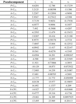
Table 8. Parameters of EOS forOil 5

nS mS

lS

Pseudocomponent

-0.17239 12.786

-8.6201

P-C10+

-5.1386 -0.08398

3.2125 N-C10+

-4.9696 -0.12094

3.2267 A-C10+

-4.5308 -0.27612

5.9567

P-C15+

-0.17938 9.9654

-5.7139 N-C15+

-0.1857 9.9896

-6.0577 A-C15+

-4.4207 -0.3908

7.492

P-C20+

-0.15433 11.679

-6.3593 N-C20+

-0.21188 10.416

-5.8307 A-C20+

-4.3724 -0.50176

8.9575

P-C25+

-0.12532 13.844

-7.4047 N-C25+

-0.22147 11.417

-6.0942 A-C25+

-4.3345 -0.6278

10.561

P-C30+

-0.098267 16.201

-8.6504 N-C30+

-0.21949 12.693

-6.588 A-C30+

-4.3053 -0.73866

11.921

P-C35+

-0.072922 18.873

-10.129 N-C35+

-0.21087 14.239

-7.2483 A-C35+

-4.2681 -0.88703

13.681

P-C40+

-0.050509 21.772

-11.777 N-C40+

-0.19855 15.977

-8.0138 A-C40+

-4.209 -1.1337

16.492

P-C46+

-0.01868 27.217

-14.927 N-CP1+

-0.1736 19.316

-9.4777 A-CP1+

0.0097925 34.309

-19.061 N-CP2+

-0.20113 23.969

30 Iranian Journal of Chemical Engineering, Vol. 5, No. 2

Table 9. Parameters of EOS for Oil 6

nS

mS

lS Pseudocomponent

-0.1522 11.668

-7.6701 P-CP1

-0.16432 7.8714

-4.7492 N-CP1

-4.7521 -0.13346

3.1885 A-CP1

-0.047253 13.428

-7.9844 P-CP2

-4.8242 -0.10604

3.8369 N-CP2

-4.8232 -0.11553

3.6483 A-CP2

-4.2186 -0.37657

6.4993 P-CP3

-0.094925 9.1252

-4.3969 N-CP3

-0.11886 8.6468

-4.3753 A-CP3

-4.1055 -0.49264

7.6419 P-CP4

-0.064131 10.188

-4.6555 N-CP4

-0.12237 8.8143

-4.0311 A-CP4

-3.8195 -1.2069

13.934 P-CP5

0.063654 17.942

-7.8951 N-CP5

-0.078385 12.168

-4.135 A-CP5

-3.754 -1.4885

16.199 P-CP6

0.090889 20.954

-9.3345 N-CP6

-0.055752 13.697

-4.4112 A-CP6

-3.7459 -1.5269

16.502 P-CP7

0.094017 21.355

-9.5289 N-CP7

-0.052763 13.904

-4.4491 A-CP7

0.1122 23.979

-10.807 N-CP8

-0.033513 15.265

-4.6938 A-CP8

S

α is independent of pressure and it can be used for the solid volume prediction [11]. It seems that the prediction errors for the lighter

components, like C10, are greater than those

for the heavy fractions.

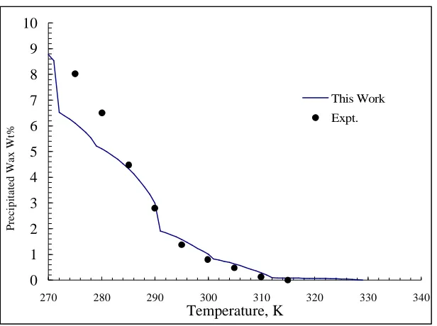
0 1 2 3 4 5 6 7 8 9 10

270 280 290 300 310 320 330 340

Temperature, K

P

re

c

ip

it

a

te

d

W

a

x

W

t%

This Work

Expt.

Iranian Journal of Chemical Engineering, Vol. 5, No. 2 31

0 2 4 6 8 10 12 14 16

270 280 290 300 310 320

Temperature (K)

P

re

ci

p

it

at

ed

W

ax

W

t%

This Work

Expt.

Figure 2. Experimental and calculated amount of precipitated wax for Oil 6

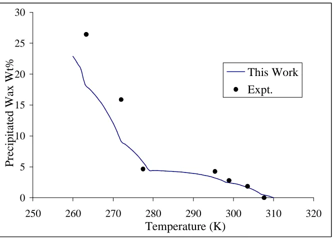
0 5 10 15 20 25 30

250 260 270 280 290 300 310 320

Temperature (K)

P

re

ci

p

it

at

ed

W

ax

W

t% _{This Work}

Expt.

32 Iranian Journal of Chemical Engineering, Vol. 5, No. 2

0 10 20 30 40 50 60

265 275 285 295 305 315

Temperature (K)

P

re

ci

p

it

at

ed

W

ax

W

t%

This Work

Expt.

Figure 4. Experimental and calculated amount of precipitated wax formixture B

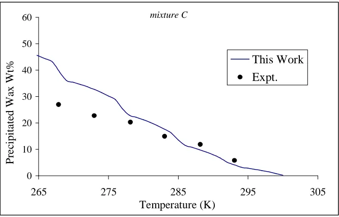
mixture C

0 10 20 30 40 50 60

265 275 285 295 305

Temperature (K)

P

re

ci

p

it

a

te

d

W

ax

W

t% This Work

Expt.

Iranian Journal of Chemical Engineering, Vol. 5, No. 2 33

Conclusion

Complex behavior of a solid phase in an oil mixture and the wide range of its application in solid precipitation and deposition petroleum fluids (wax, asphaltene, …) need to be modeled via applicable and efficient methods. Here, the application of a solid EOS for the description of solid phase was tested for wax precipitation in petroleum mixtures. In this work, TST solid equation of state is used for describing wax precipitation phenomena in some synthetic and real oil mixtures. This solid equation of state is based on an alpha function. Using thermodynamic method for pure solid fugacity from pure liquid fugacity, the TST EOS parameters were tuned before its application for wax precipitation prediction. The multisolid phase approach is used for determination of the nature and number of solid phases. As can be seen in the previous sections, the obtained results in this work are in good agreement with the experimental data.

References

1. Won, K. V. "Thermodynamics Calculation of Cloud Point Temperatures and Wax Phase Composition of Refined Hydrocarbon Mixtures," Fluid Phase Equilibria, 53, 377 (1989).

2. Won, K. V. "Thermodynamics for Solid Solition-Liquid-Vapor Equilibria: Wax Formation From Heavy Hydrocarbon Mixtures," Fluid Phase Equilibria, 30, 265, (1986).

3. Daridon, J. L., Pauly, J., Coutinho, J. A. P. and Montel, F. "Solid-Liquid-Vapor Phase Boundary of a North Sea Waxy Crude: Measurement and Modeling," Energy and

Fuels, 15, 730, (2001).

4. Coutinho, J. A. P. and Daridon, J. L. "Low-Pressure Modeling of Wax Formation in Crude Oils," Energy and Fuels, 15, 1454 (2001).

5. Vafaei-Sefti, M., Mousavi-Dehghani, S. A. and Mohammad-Zadeh Bahar, M. "Modi-fication of multi solid phase model for prediction of wax precipitation: a new and effective solution method," Fluid Phase

Equilibria, 173, 65, (2000).

6. Nichita, D. V., Gousl, L. and Firoozabadi, A. "Wax Precipitation in Gas Condensate Mixtures," SPE 74686, (2001).

7. Dalirsefat, R. and Feyzi, F. "A thermo-dynamic model for wax deposition phenomena," Fuel, 86, 1402 (2007).

8. Lira-Galeana, C., Firoozabadi, A. and Prausnitz, J. M. "Thermodynamics of Wax Precipitation in Petroleum Mixtures," AIChE,

42, 239 (1996).

9. Coutinho, J. A. P., Edmonds, B., Moorwood, T., Szczepanski, R. and Zhang, X. "Reliable Wax Predictions for Flow Assurance," SPE 78324, (2002).

10.Yokozeki, A. "Analytical Equation of State for Solid -Liquid-Vapor Phases,"

Inter-national Journal of Thermophysics, 24, 589

(2003).

11.Twu, C. H., Tassone, V. and Sim, W. D. "New Solid Equation of State Combining Excess Energy Mixing Rule for Solid Liquid Equilibria," AIChEJ, 49, 2957 (2003).

12.Ness, H. C. V. and Abbott, M. H., "Classical Thermodynamics of Non-Electrolyte Solu-tions with Application tp Phase Equilibria," New York: Mc-Graw Hill, (1982).

13.Prausnitz, J., Lichtenthaler, M. R. N. and de Azevedo, E.G., "Molecular Thermodynamics of Fluid-Phase Equilibria," Upper Saddle River, New Jersey: Printice Hall, (1999). 14.Escobar-Remolina, J. C. M. "Prediction of

characteristics of wax precipitation in synthetic mixtures and fluids of petroleum: A new model," Fluid Phase Equilibria, 240, 197 (2006).

15.Powell, M. J. D. "A Fortran Subroutine for Solving Systems of Nonlinear Algebraic Equations," Numerical Methods for Nonl-inear Algebraic Equations, P. Rabinowitz, Ch.7, (1970)