A View of Margin Losses as Regularizers of Probability Estimates

A View of Margin Losses as Regularizers of Probability

Estimates

Hamed Masnadi-Shirazi [email protected]

School of Electrical and Computer Engineering, Shiraz University,

Shiraz, Iran

Nuno Vasconcelos [email protected]

Statistical Visual Computing Laboratory, University of California, San Diego La Jolla, CA 92039, USA

Editor:Saharon Rosset

Abstract

Regularization is commonly used in classifier design, to assure good generalization. Clas-sical regularization enforces a cost on classifier complexity, by constraining parameters. This is usually combined with a margin loss, which favors large-margin decision rules. A novel and unified view of this architecture is proposed, by showing that margin losses act as regularizers of posterior class probabilities, in a way that amplifies classical parameter regularization. The problem of controlling the regularization strength of a margin loss is considered, using a decomposition of the loss in terms of a link and a binding function. The link function is shown to be responsible for the regularization strength of the loss, while the binding function determines its outlier robustness. A large class of losses is then categorized into equivalence classes of identical regularization strength or outlier robust-ness. It is shown that losses in the same regularization class can be parameterized so as to have tunable regularization strength. This parameterization is finally used to derive boost-ing algorithms with loss regularization (BoostLR). Three classes of tunable regularization losses are considered in detail. Canonical losses can implement all regularization behav-iors but have no flexibility in terms of outlier modeling. Shrinkage losses support equally parameterized link and binding functions, leading to boosting algorithms that implement the popular shrinkage procedure. This offers a new explanation for shrinkage as a special case of loss-based regularization. Finally,α-tunable losses enable the independent parame-terization of link and binding functions, leading to boosting algorithms of great flexibility. This is illustrated by the derivation of an algorithm that generalizes both AdaBoost and LogitBoost, behaving as either one when that best suits the data to classify. Various exper-iments provide evidence of the benefits of probability regularization for both classification and estimation of posterior class probabilities.

1. Introduction

The ability to generalize beyond the training set is a central challenge for classifier design. A binary classifier is usually implemented by thresholding a continuous function, the classifier predictor, of a high-dimensional feature vector. Predictors are frequently affine functions, whose level sets (decision boundaries) are hyperplanes in feature space. Optimal predictors minimize the empirical expectation of a loss function, or risk, on a training set. Modern risks guarantee good generalization by enforcing large margins and parameter regularization. Large margins follow from the use of margin losses, such as the hinge loss of the support vector machine (SVM), the exponential loss of AdaBoost, or the logistic loss of logistic regression and LogitBoost. These are all upper-bounds on the zero-one classification loss of classical Bayes decision theory. Unlike the latter, margin losses assign a penalty to examples correctly classified but close to the boundary. This guarantees a classification margin and improved generalization (Vapnik, 1998). Regularization is implemented by penalizing predictors with many degrees of freedom. This is usually done by augmenting the risk with a penalty on the norm of the parameter vector. Under a Bayesian interpretation of risk minimization, different norms correspond to different priors on predictor parameters, which enforce different requirements on the sparseness of the optimal solution.

While for some popular classifiers, e.g. the SVM, regularization is a natural side-product of risk minimization under a margin loss (Moguerza and Munoz, 2006; Chapelle, 2007; Huang et al., 2014), the relation between the two is not always as clear for other learning methods, e.g. boosting. Regularization can be added to boosting (Buhlmann and Hothorn, 2007; Lugosi and Vayatis, 2004; Blanchard et al., 2003) in a number of ways, including re-stricting the number of boosting iterations (Raskutti et al., 2014; Natekin and Knoll, 2013; Zhang and Yu, 2005; Rosset et al., 2004; Jiang, 2004; Buhlmann and Yu, 2003), adding a regularization term (Saha et al., 2013; Culp et al., 2011; Xiang et al., 2009; Bickel et al., 2006; Xi et al., 2009), restricting the weight update rule (Lozano et al., 2014, 2006; Lugosi and Vayatis, 2004; Jin et al., 2003) or using divergence measures (Liu and Vemuri, 2011) and has been implemented for both the supervised and semi-supervised settings (Chen and Wang, 2008, 2011). However, many boosting algorithms lack explicit parameter regular-ization. Although boosting could eventually overfit (Friedman et al., 2000; Rosset et al., 2004), and there is an implicit regularization when the number of boosting iterations is limited (Raskutti et al., 2014; Natekin and Knoll, 2013; Zhang and Yu, 2005; Rosset et al., 2004; Jiang, 2004; Buhlmann and Yu, 2003), there are several examples of successful boost-ing on very high dimensional spaces, usboost-ing complicated ensembles of thousands of weak learners, and no explicit regularization (Viola and Jones, 2004; Schapire and Singer, 2000; Viola et al., 2003; Wu and Nevatia, 2007; Avidan, 2007). This suggests that regularization is somehow implicit in large margins, and additional parameter regularization may not always be critical, or even necessary. In fact, in domains like computer vision, large margin classi-fiers are more popular than classiclassi-fiers that enforce regularization but not large margins, e.g. generative models with regularizing priors. This suggests that the regularization implicit in large margins is complementary to parameter regularization. However, this connection has not been thoroughly studied in the literature.

mini-mization: the loss φ, the minimum risk C_φ∗, and a link function f_φ∗ that maps posterior class probabilities to classifier predictions (Friedman et al., 2000; Zhang, 2004; Buja et al., 2006; Masnadi-Shirazi and Vasconcelos, 2008; Reid and Williamson, 2010). We consider the subset of losses of invertible link, since this enables the recovery of class posteriors from predictor outputs. Losses with this property are known as proper losses and important for applications that require estimates of classification confidence, e.g. multiclass decision rules based on binary classifiers (Zadrozny, 2001; Rifkin and Klautau, 2004; Gonen et al., 2008; Shiraishi and Fukumizu, 2011). We provide a new interpretation of these losses as regularizers of finite sample probability estimates and show that this regularization has at least two important properties for classifier design. First, it combines multiplicatively with classical parameter regularization, amplifying it in a way that tightens classification error bounds. Second, probability regularization strength is proportional to loss margin for a large class of link functions, denoted generalized logit links. This enables the introduction of tunable regularization losses φσ, parameterized by a probability regularization gain σ.

A procedure to derive boosting algorithms of tunable loss regularization (BoostLR) from these losses is also provided. BoostLR algorithms generalize the GradientBoost procedure (Friedman, 2001), differing only in the example weighting mechanism, which is determined by the lossφσ.

To characterize the behavior of these algorithms, we study the spaceRof proper lossesφ

of generalized logit link. It is shown that any suchφis uniquely defined by two components: the link f_φ∗ and a binding function βφ that maps f_φ∗ into the minimum risk C_φ∗. This

decomposition has at least two interesting properties. First, the two components have a functional interpretation: whilef_φ∗ determines the probability regularization strength of φ, βφ determines its robustness to outliers. Second, bothβφand f_φ∗ define equivalence classes

inR. It follows that Rcan be partitioned into subsets of losses that have either the same outlier robustness or probability regularization properties. It is shown that the former are isomorphic to a set of symmetric scale probability density functions and the latter to the set of monotonically decreasing odd functions. Three loss classes, with three different binding functions, are then studied in greater detail. The first, the class of canonical losses, consists of losses of linear binding function. This includes some of the most popular losses in the literature, e.g. the logistic. While they can implement all possible regularization behaviors, these losses have no additional degrees of freedom. In this sense, they are the simplest tunable regularization losses. This simplicity enables a detailed analytical characterization of their shape and how this shape is affected by the regularization gain. The second, the class of shrinkage losses, is a superset of the class of canonical losses. Unlike their canonical counterparts, shrinkage losses support nonlinear binding functions, and thus more sophisticated handling of outliers. However, they require an identical parameterization of the link and binding function. It is shown that, under this constraint, BoostLR implements the popular shrinkage regularization procedure (Hastie et al., 2001). Finally, the class of

The paper is organized as follows. Section 2 briefly reviews classifier design by risk mini-mization. The view of margin losses as regularizers of probability estimates is introduced in Section 3. Section 4 characterizes the regularization strength of proper losses of generalized logit link. Tunable regularization losses and binding functions are introduced in Section 5, which also introduces the BoostLR algorithm. The structure of R is then characterized in Section 6, which introduces canonical, shrinkage, and α-tunable losses. An extensive set of experiments on various aspects of probability regularization is reported in Section 7. Finally, some conclusions are drawn in Section 8.

2. Loss Functions and Risk Minimization

We start by reviewing the principles of classifier design by risk minimization (Friedman et al., 2000; Zhang, 2004; Buja et al., 2006; Masnadi-Shirazi and Vasconcelos, 2008) .

2.1 The Classification Problem

A classifierh maps a feature vector x∈ X to a class label y∈ {−1,1}, according to

h(x) =sign[p(x)], (1)

where p : X → _R is the classifier predictor. Feature vectors and class labels are drawn from probability distributionsPX(x) andPY|X(y|x) respectively. Given a non-negative loss

functionL(x, y), the optimal predictor p∗(x) minimizes the risk

R(p) =EX,Y[L(p(x), y)]. (2)

This is equivalent to minimizing the conditional risk

EY|X[L(p(x), y)|X=x]

for all x∈ X. It is frequently useful to expressp(x) as a composition of two functions,

p(x) =f(η(x)),

where η(x) = PY|X(1|x) is the posterior probability function, and f : [0,1] → R a link function. The problem of learning the optimal predictor can thus be decomposed into the problems of learning the optimal linkf∗(η) and estimating the posterior functionη(x). Since

f∗(η) can usually be determined analytically, this reduces to estimating η(x), whenever

f∗(η) is a one-to-one mapping.

In classical statistics, learning is usually based on the zero-one loss

L_0/1(y, p) = 1−sign(yp)

2 =

0, ify=sign(p); 1, ify6=sign(p),

where we omit the dependence on x for notational simplicity. The associated conditional risk

C0/1(η, p) =η

1−sign(p)

2 + (1−η)

1 +sign(p)

2 =

1−η, ifp=f(η)≥0;

is the probability of error of the classifier of (1), and is minimized by anyf∗ such that







f∗(η)>0 ifη > 1₂ f∗(η) = 0 ifη= 1₂

f∗(η)<0 ifη < 1₂.

(3)

The optimal classifier h∗(x) = sign[p∗(x)], where p∗ = f∗(η), is the well known Bayes decision rule, and has minimum conditional (zero-one) risk

C_0/1∗ (η) =η

1 2 −

1

2sign(2η−1)

+ (1−η)

1 2 +

1

2sign(2η−1)

= min{η,1−η}.

2.2 Learning from Finite Samples

Practical learning algorithms produce an estimate ˆp∗(x) of the optimal predictor by min-imizing an empirical estimate of (2), the empirical risk, from a training sample D = {(x1, y1), . . . ,(xn, yn)}

Remp(p) =

1

n

X

i

L(p(xi), yi). (4)

This can be formulated as fitting a model ˆη(x) = [f∗]−1(p(x;w)) to the sampleD, wheref∗

is an invertible link that satisfies (3) and p(x;w) a parametric predictor. Two commonly used links are

f∗= 2η−1 and f∗ = log η 1−η.

In this way, the learning problem is reduced to the estimation of the model parameterswof minimum empirical risk. Most modern learning techniques rely on a linear predictor, imple-mented on eitherX -p(x,w) =wT_{x- or some transformed space -p(x,w) =w}T_{Φ(x). For}

example, logistic regression (Hosmer and Lemeshow, 2000) uses the logit linkf∗ = log₁₋η_η, or equivalently the logistic inverse link [f∗]−1(v) = _1+eevv, and learns a linear predictor

p(x,w) = wTx. When a transformation Φ(x) is used, it is either implemented indi-rectly with recourse to a kernel function, e.g. kernelized logistic regression (Zhu and Hastie, 2001), or learned. For example, boosting algorithms rely on a transformation Φ(x) = (h1(x), . . . , hm(x)) wherehi(x) is a weak or base classifier selected during training.

In this case, the predictor has the form

p(x;w) =X

i

wihi(x). (5)

In all cases, given the optimal predictor estimate ˆp∗(x) = p(x,w∗), estimates of the posterior probability η(x) can be obtained with ˆη(x) = [f∗]−1_(ˆp∗_{(x)). However, when} learning is based on the empirical risk of (4), convergence to the true probabilities is only guaranteed asymptotically and for certain loss functionsL(., .). Even when this is the case, learning algorithms can easily overfit to the training set, for finite samples. The minimum of (4) is achieved for some empirical predictor

ˆ

−4 −3 −2 −1 0 1 2 3 4 0

1 2 3 4 5 6

v

µ

φ

φ(v)

−4 −3 −2 −1 0 1 2 3 4 0

0.1 0.2 0.3 0.4 0.5 0.6 0.7 0.8 0.9 1

v [f*

φ]

−1_(v)

{[f*

φ]

−1_}′(v)

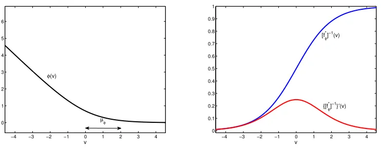
Figure 1: Left: A margin loss function (the logistic loss) of margin parameter µφ, defined

in (25). Right: corresponding inverse link (in blue) and its growth rate (in red).

wherep∗(x) is the optimal predictor andp(x) a prediction error, sampled from a zero mean

distribution of decreasing variance with sample size. For a given sample size, a predictor with error of smaller variance is said to generalize better. One popular mechanism to prevent overfitting is to regularize the parameter vector w, by imposing a penalty on its norm, i.e. minimizing

Remp(p) =

1

n

X

i

L(p(xi), yi) +λ||w||l

instead of (4). We refer to this as parameter regularization.

2.3 Margin Losses

Another possibility is to change the loss function, e.g. by replacing the 0-1 loss with a margin loss Lφ(y, p(x)) = φ(yp(x)). As illustrated in Figure 1 (left), these losses assign a

non-zero penalty to small positive values of the marginyp, i.e. in the range 0 < yp < µφ,

where µφ is a parameter, denoted the loss margin. Commonly used margin losses include

the exponential loss of AdaBoost, the logistic loss (shown in the figure) of logistic regression, and the hinge loss of SVMs. The resulting large-margin classifiers have better finite sample performance (generalization) than those produced by the 0-1 loss (Vapnik, 1998). The associated conditional risk

Cφ(η, p) =Cφ(η, f(η)) =ηφ(f(η)) + (1−η)φ(−f(η)) (7)

is minimized by the link

f_φ∗(η) = arg min

f Cφ(η, f) (8)

leading to the minimum conditional risk function

Algorithm φ(v) f_φ∗(η) [f_φ∗]−1(v) C_φ∗(η)

SVM max(1−v,0) sign(2η−1) NA 1− |2η−1|

Boosting exp(−v) 1₂log₁₋η_{η 1+e}e2v2v 2

p

η(1−η)

Logistic Regression log(1 +e−v) log₁₋η_{η 1+e}evv -ηlogη−(1−η) log(1−η)

Table 1: Loss φ, optimal link f_φ∗(η), optimal inverse link [f_φ∗]−1(v) , and minimum condi-tional risk C_φ∗(η) of popular learning algorithms.

Unlike the 0-1 loss, the optimal link is usually unique for margin losses and computable in closed-form, by solvingηφ0(f_φ∗(η)) = (1−η)φ0(−f_φ∗(η)) forf_φ∗. Table 1 lists the loss, optimal link, and minimum risk of popular margin losses.

The adoption of a margin loss can be equivalent to the addition of parameter reg-ularization. For example, a critical step of the SVM derivation is a normalization that makes the margin identical to 1/||w||, where w is the normal of the SVM hyperplane

p(x;w) =wTx (Moguerza and Munoz, 2006; Chapelle, 2007). This renders margin maxi-mization identical to the minimaxi-mization of hyperplane norm, leading to the interpretation of the SVM as minimizing the hinge loss under a regularization constraint on w (Moguerza and Munoz, 2006; Chapelle, 2007), i.e.

RSV M(w) =

1

n

X

i

max[0,1−yp(xi;w)] +λ||w||2. (10)

In this case, larger margins translate directly into the regularization of classifier parameters. This does not, however, hold for all large margin learning algorithms. For example, boosting does not use explicit parameter regularization, although regularization is implicit in early stopping (Raskutti et al., 2014; Natekin and Knoll, 2013; Zhang and Yu, 2005; Rosset et al., 2004; Jiang, 2004; Buhlmann and Yu, 2003). This consists of terminating the algorithm after a small number of iterations. While many bounds have been derived to characterize the generalization performance of large margin classifiers, it is not always clear how much of the generalization ability is due to the loss vs. parameter regularization. In what follows, we show that margin losses can themselves be interpreted as regularizers. However, instead of regularizing predictor parameters, they directly regularize posterior probability estimates, by acting on the predictor output. This suggests a complementary role for loss-based and parameter regularization. We will see that the two types of regularization in fact have a multiplicative effect.

3. Proper Losses and Probability Regularization

3.1 Regularization Losses

For any margin loss whose link of (8) is invertible, posterior probabilities can be recovered from

η(x) = [f_φ∗]−1(p∗(x)). (11) Whenever this is the case, the loss is said to be proper1 and the predictor calibrated (De-Groot and Fienberg, 1983; Platt, 2000; Niculescu-Mizil and Caruana, 2005; Gneiting and Raftery, 2007). For finite samples, estimates of the probabilitiesη(x) are obtained from the empirical predictor ˆp∗ with

ˆ

η(x) = [f_φ∗]−1(ˆp∗(x)). (12) Parameter regularization improves estimates ˆp∗(x) by constraining predictor parameters. For example, a linear predictor estimate ˆp∗(x; ˆw) = ˆwTxcan be written in the form of (6), with p∗(x) = w∗Tx and p(x) = wTx, where w is a parameter estimation error. The

regularization of (10) reduces w and the prediction error p(x), improving probability

estimates in (12).

Loss-based regularization complements parameter regularization, by regularizing the probability estimates directly. To see this note that, whenever the loss is proper and the noise component p of (6) has small amplitude, (12) can be approximated by its Taylor

series expansion aroundp∗

ˆ

η(x) ≈ [f_φ∗]−1(p∗(x)) +{[f_φ∗]−1}0(p∗(x))p(x)

= η(x) +η(x)

with

η(x) ={[fφ∗]

−1_}0_(p∗_(x))

p(x). (13)

If|{[f_φ∗]−1}0(p∗(x))|<1 the probability estimation noiseη has smaller magnitude than the

prediction noisep. Hence, for equivalent prediction errorp, a lossφwith inverse link [fφ∗]−1

of smaller growth rate|{[f_φ∗]−1}0(v)|produces more accurate probability estimates. Figure 1 (right) shows the growth rate of the inverse link of the logistic loss. When the growth rate is smaller than one, the loss acts as a regularizer of probability estimates. From (13), this reg-ularization multiplies any decrease of prediction error obtained by parameter regreg-ularization. This motivates the following definition.

Definition 1 Let φ(v) be a proper margin loss. Then

ρφ(v) =

1

|{[f_φ∗]−1_}0_(v)| (14)

is the regularization strength ofφ(v). Ifρφ(v)≥1,∀v,thenφ(v)is denoted a regularization loss.

3.2 Generalization

An alternative way to characterize the interaction of loss-based and parameter-based regu-larization is to investigate how the two impact classifier generalization. This can be done by characterizing the dependence of classification error bounds on the two forms of regular-ization. Since, in this work, we will emphasize boosting algorithms, we rely on the following well known boosting bound.

Theorem 1 (Schapire et al., 1998) Consider a sampleS ofmexamples{(x1, yi), . . . ,(xm, ym)} and a predictor pˆ∗(x;w) of the form of (5) where the hi(x) are in a space H of base classi-fiers of VC-dimension d. Then, with probability at least1−δ over the choice of S, for all θ >0,

PX,Y[yp(x;w)≤0]≤PS

ypˆ∗(x;w) ||w||1 ≤θ +O   1 √ m s

dlog2(m/d)

θ2 + log(1/δ)



,

where PS denotes an empirical probability over the sample S.

GivenH, m, dandδ, the two terms of the bound are functions ofθ. The first term depends on the distribution of the marginsyipˆ∗(xi;w) over the sample. Assume, for simplicity, that S is separable by ˆp∗(x;w), i.e. yipˆ∗(xi;w)>0,∀i, and denote the empirical margin by

γs =yi∗pˆ∗(x_i∗;w), i∗= arg min

i yipˆ

∗_(x

i;w). (15)

Then, for any >0 andθ=γs/||w||1−, the empirical probability is zero and

PX,Y[yp(x;w)≤0]≤O

1 √

m

s

dlog2(m/d) ( γs

||w||1 −)

2 + log(1/δ)

!

.

Using (11) and a first order Taylor series expansion of [f_φ∗]−1(.) around the origin ˆ

η(xi∗) = [f∗

φ]

−1_(y i∗γ_s)

≈ [f_φ∗]−1(0) +yi∗γ_s{[f∗

φ]

−1_}0₍₀₎ it follows that

γs≈ρφ(0)|ηˆ(xi∗)−1/2|, (16)

and the bound can be approximated by

PX,Y[yp(x;w)≤0]≤O

    1 √ m v u u u t

dlog2(m/d)

_ρ

φ(0) ||w||1|ηˆ(xi

∗)−1/2| −

2 + log(1/δ) 

  

. (17)

Since this is a monotonically decreasing function of the generalization factor

κ= ρφ(0)

largerκ lead to tighter bounds on the probability of classification error, i.e. classifiers with stronger generalization guarantees. This confirms the complimentary nature of parameter and probability regularization, discussed in the previous section. Parameter regularization, as in (10), encourages solutions of smaller ||w||₁ and thus larger κ. Regularization losses multiply this effect by the regularization strength ρφ(0). This is in agreement with the

multiplicative form of (13). In summary, for regularization losses, the generalization guar-antees of classical parameter regularization are amplified by the strength of the probability regularization at the classification boundary.

4. Controlling the Regularization Strength of Proper Losses

In the remainder of this work, we study the design of regularization losses. In particular, we study how to control the regularization strength of a proper loss, by manipulating some loss parameter.

4.1 Proper Losses

The structure of proper losses can be studied by relating conditional risk minimization to the classical problem of probability elicitation in statistics (Savage, 1971; DeGroot and Fienberg, 1983). Here, the goal is to find the probability estimator ˆη that maximizes the expected score

I(η,ηˆ) =ηI1(ˆη) + (1−η)I−1(ˆη), (19)

of a scoring rule that assigns to prediction ˆη a score I1(ˆη) when event y = 1 holds and a

scoreI−1(ˆη) wheny =−1 holds. The scoring rule is proper if its components I1(·), I−1(·)

are such that the expected score is maximal when ˆη=η, i.e.

I(η,ηˆ)≤I(η, η) =J(η), ∀η (20)

with equality if and only if ˆη =η. A set of conditions under which this holds is as follows.

Theorem 2 (Savage, 1971) LetI(η,ηˆ)be as defined in (19) andJ(η) =I(η, η). Then (20) holds if and only if J(η) is convex and

I1(η) =J(η) + (1−η)J0(η) I−1(η) =J(η)−ηJ0(η). (21)

Several works investigated the connections between probability elicitation and risk mini-mization (Buja et al., 2006; Masnadi-Shirazi and Vasconcelos, 2008; Reid and Williamson, 2010). We will make extensive use of the following result.

Theorem 3 (Masnadi-Shirazi and Vasconcelos, 2008) Let I1(·) and I−1(·) be as in (21), for any continuously differentiable convex J(η) such that J(η) = J(1−η), and f(η) any invertible function such that f−1(−v) = 1−f−1(v). Then

I1(η) =−φ(f(η)) I−1(η) =−φ(−f(η)) if and only if

It has been shown that, forCφ(η, p), fφ∗(η),andCφ∗(η) as in (7)-(9),Cφ∗(η) is concave (Zhang,

2004) and

C_φ∗(η) = C_φ∗(1−η) (22)

[f_φ∗]−1(−v) = 1−[f_φ∗]−1(v). (23) Hence, the conditions of the theorem are satisfied by any continuously differentiableJ(η) = −C_φ∗(η) and invertible f(η) = f_φ∗(η). It follows that, I(η,ηˆ) = −Cφ(η, f) is the expected

score of a proper scoring rule if and only if the loss has the form

φ(v) =C_φ∗ [f_φ∗]−1(v)+ (1−[f_φ∗]−1(v))[C_φ∗]0 [f_φ∗]−1(v). (24) In this case, the predictor of minimum risk is p∗ =f_φ∗(η), and posterior probabilities can be recovered with (11). Hence, the loss φ is proper and the predictor p∗ calibrated. In summary, proper losses have the structure of (22)-(24). In this work, we also assume that

C_φ∗(0) =C_φ∗(1) = 0. This guarantees that the minimum risk is zero when there is absolute certainty about the class label Y, i.e. PY|X(1|x) = 0 or PY|X(1|x) = 1.

4.2 Loss Margin and Regularization Strength

The facts that 1) the empirical margin γs of (15) is a function of the loss margin µφ of

Figure 1, and 2) the regularization strengthρφis related toγsby (16), suggests thatµφis a

natural loss parameter to controlρφ. A technical difficulty is that a universal definition of µφis not obvious, since most margin lossesφ(v) only converge to zero asv→ ∞. Although

approximately zero for large positivev, they are strictly positive for all finitev. This is, for example, the case of the logistic loss φ(v) = log(1 +e−v_{) of Figure 1 and the boosting loss}

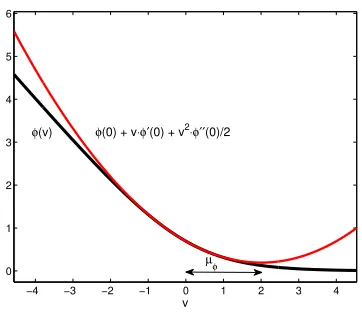
of Table 1. To avoid this problem, we use a definition based on the second-order Taylor series expansion ofφaround the origin. The construct is illustrated in Figure 2, where the loss marginµφis defined by the point where the quadratic expansion reaches its minimum.

It can be easily shown that this is the pointv =µφ, where

µφ=− φ0(0)

φ00(0). (25)

In Appendix A, we show that, under mild conditions (see Lemma 9) on the inverse link [f_φ∗]−1_{(η) of a twice differentiable loss φ}

µφ= ρφ(0)

2 , (26)

and the regularization strength ofφis lower bounded by twice the loss margin

ρφ(v)≥2µφ. (27)

Under these conditions,φ(v) is a regularization loss if and only ifµφ≥ 1₂. This establishes

a direct connection between margins and probability regularization: larger loss margins produce more strongly regularized probability estimates. Hence, for proper losses of suitable link, the large margin strategy for classifier learning is also a strategy for regularization of probability estimates. In fact, from (26) and (18), the generalization factor of these losses is directly determined by the loss margin, since κ= 2µφ

−4 −3 −2 −1 0 1 2 3 4 0

1 2 3 4 5 6

v

φ(v) φ(0) + v⋅φ′(0) + v2⋅φ′′(0)/2

µ

φ

Figure 2: Definition of the loss marginµφ of a lossφ.

4.3 The Generalized Logit Link

As shown in Lemma 9 of Appendix A, the conditions that must be satisfied by the inverse link for (26) and (27) to hold (monotonically increasing, maximum derivative at the origin) are fairly mild. For example, they hold for the scaled logit

γ(η;a) =alog η

1−η γ

−1_{(v;a) =} ev/a

1 +ev/a, (28)

which, as shown in Table 1, is the optimal link of the exponential loss when a = 1/2 and of the logistic loss when a= 1. Since the exponential loss of boosting has margin µφ = 1

and the logistic loss µφ= 2, it follows from the lemma that these are regularization losses.

However, the conditions of the lemma hold for many other link functions. In this work, we consider a broad family of such functions, which we denote as the generalized logit.

Definition 2 An invertible transformationπ(η) is a generalized logit if its inverse,π−1_(v), has the following properties

1. π−1(v) is monotonically increasing, 2. limv→∞π−1(v) = 1

3. π−1_{(−v) = 1−π}−1_(v),

4. for finite v, (π−1₎(2)_{(v) = 0 if and only if v = 0,} where π(n) is the nth order derivative of π.

Theorem 4 Let φ(v) be a twice differentiable proper loss of generalized logit link f_φ∗(η). Then

µφ= ρφ(0)

2 (29)

and the regularization strength ofφ(v)is lower bounded by twice the loss marginρφ(v)≥2µφ. φ(v) is a regularization loss if and only if µφ≥ 1₂.

5. Controlling the Regularization Strength

The results above show that it is possible to control the regularization strength of a proper loss of generalized logit link by manipulating the loss margin µφ. In this section we derive

procedures to accomplish this.

5.1 Tunable Regularization Losses

We start by studying the set of proper margin losses whose regularization is controlled by a parameter σ >0. These are denoted tunable regularization losses.

Definition 3 Let φ(v) be a proper loss of generalized logit link f_φ∗(η). A parametric loss

φσ(v) =φ(v;σ) such that φ(v; 1) =φ(v)

is the tunable regularization loss generated by φ(v) if φσ(v) is a proper loss of generalized logit link and

µφσ =σµφ,

for all σ such that

σ≥ 1 2µφ

. (30)

The parameterσ is the gain of the tunable regularization loss φσ(v).

Since, from (29) and (14), the loss marginµφonly depends on the derivative of the inverse

link at the origin, a tunable regularization loss can be generated from any proper loss of generalized logit link, by simple application of Theorem 3.

Lemma 4 Let φ(v) be a proper loss of generalized logit link f_φ∗(η). The parametric loss

φσ(v) =Cφ∗σ{[f ∗

φσ]

−1_{(v)}+ (1−[f}∗

φσ]

−1_(v))[C∗

φσ] 0

([f_φ∗_σ]−1(v)), (31)

where

f_φ∗_σ(η) = σf_φ∗(η) (32)

C_φ∗

σ(η)is a minimum risk function (i.e. a continuously differentiable concave function with

Proof From (32)

[f_φ∗_σ]−1(v) = [f_φ∗]−1

v

σ

. (33)

Since [f_φ∗]−1_{(v) is a generalized logit link it has the properties of Definition 2. Since these}

properties continue to hold whenv is replaced byv/σ, it follows thatf_φ∗_σ(v) is a generalized logit link. It follows from (31) that φσ(v) satisfies the conditions of Theorem 3 and is a

proper loss. Sinceµφσ =

ρφσ(0)

2 =

1

2{[f_φσ∗ ]−1_}0₍₀₎ =σµφ, the parametric lossφσ(v) is a tunable

regularization loss.

In summary, it is possible to generate a tunable regularization loss by simply rescaling the link of a proper loss. Interestingly, this holds independently of how σ parameterizes the minimum risk [C_φ∗

σ](η). However, not all such losses are useful. If, for example, the process results in

φσ(v) =φ(v/σ),

it corresponds to a simple rescaling of the horizontal axis of Figure 1. The lossφσ(v) is thus

not fundamentally different fromφ(v). Using this loss in a learning algorithm is equivalent to varying the margin by rescaling the feature spaceX.

5.2 The Binding Function

To produce non-trivial tunable regularization lossesφσ(v), we need a better understanding

of the role of the minimum risk [C_φ∗

σ](η). This is determined by the binding function of the loss.

Definition 5 Let φ(v) be a proper loss of link f_φ∗(η), and minimum riskC_φ∗(η). The func-tion

βφ(v) = [Cφ∗]0 [fφ∗]−1(v)

(34)

is denoted the binding function of φ.

The properties of the binding function are discussed in Appendix C and illustrated in Figure 3. For proper losses of generalized logit link, βφ(v) is a monotonically decreasing

odd function, which determines the behavior of φ(v) away from the origin and defines a one-to-one mapping between the link f_φ∗ and the derivative of the risk C_φ∗. In this way,βφ

“binds” link and risk.

The following result shows that the combination of link and binding function determine the loss up to a constant.

Theorem 5 Let φ(v) be a proper loss of generalized logit link f_φ∗(η) and binding function βφ(v). Then

φ0(v) = (1−[f_φ∗]−1(v))β_φ0(v). (35) Proof From (24) and the definition of βφ,

φ(v) =C_φ∗([f_φ∗]−1(v)) + (1−[f_φ∗]−1(v))βφ(v). (36)

1

[C*

φ]’(η) 5

−5

f*

φ(η)

f*

φ(η)

0.5 β

φ[f

*

φ(η)] 5

η

η

0.5 v

v

η

0.5

0

η

Figure 3: Link f_φ∗(η), risk derivative [C_φ∗]0(η), and binding function βφ(fφ∗(η)) of a proper

lossφ(v) of generalized logit link.

This result enables the derivation of a number of properties of proper losses of gener-alized logit link. These are discussed in Appendix D.1, where such losses are shown to be monotonically decreasing, convex under certain conditions on the inverse link and binding function, and identical to the binding function for large negative margins. In summary, a proper loss of generalized logit link can be decomposed into two fundamental quantities: the inverse link, which determines its regularization strength, and the binding function, which determines its behavior away from the origin. Since tunable regularization losses are proper, the combination of this result with Lemma 4 and Definition 5 proves the following theorem.

Theorem 6 Let φ(v) be a proper loss of generalized logit link f_φ∗(η). The parametric loss

φ0_σ(v) = (1−[f_φ∗_σ]−1(v))β_φ0_σ(v), (37)

where

f_φ∗_σ(η) = σf_φ∗(η), (38)

βφσ(v) is a binding function (i.e. a continuously differentiable, monotonically decreasing,

Algorithm 1: BoostLR

Input: Training setD={(x1, y1), . . . ,(xn, yn)}, where yi∈ {1,−1}is the class label of example

x, regularization gainσ, and numberT of weak learners in the final decision rule.

Initialization:SetG(0)_(x

i) = 0 andw(1)(xi) =−

1−[f_φ∗

σ]

−1_(y

iG(0)(xi))

β0_φ

σ yiG

(0)_(x i)

∀xi .

fort={1, . . . , T} do

choose weak learner

g∗(x) = arg max g(x)

n X

i=1

yiw(t)(xi)g(xi)

update predictor G(x)

G(t)(x) =G(t−1)(x) +g∗(x)

update weights

w(t+1)(xi) =−1−[f_φ∗_σ]−1(yiG(t)(xi))β_φ0_σyiG(t)(xi) ∀xi

end for

Output: decision rule h(x) = sgn[G(T)_(x)].

5.3 Boosting With Tunable Probability Regularization

Given a tunable regularization lossφσ, various algorithms can be used to design a classifier.

Boosting accomplishes this by gradient descent in a space W of weak learners. While there are many variants, in this work we adopt the GradientBoost framework (Friedman, 2001). This searches for the predictor G(x) of minimum empirical risk on a sample D = {(x1, y1), . . . ,(xn, yn)},

R(G) =

n

X

i=1

φσ(yiG(xi)).

At iterationt, the predictor is updated according to

G(t)(x) =G(t−1)(x) +g(t)(x), (39) whereg(t)_{(x) is the gradient ofR(G) in W, i.e. the weak learner}

g(t)(x) = arg max

g n

X

i=1

−yiφ0σ(yiG(t−1)(xi))g(xi)

= arg max

g n

X

i=1

yiw(t)σ (xi)g(xi),

where

is the weight of examplexi at iterationt. For a tunable regularization loss φσ(v) of

gener-alized logit link f_φ∗_σ(η) and binding function βφσ(v), it follows from (37) that

w(t)_σ (xi) =−

1−[f_φ∗_σ]−1

yiG(t−1)(xi)

β0_φσ

yiG(t−1)(xi)

. (40)

Boosting with these weights is denoted boosting with loss regularization (BoostLR) and summarized in Algorithm 1.

The weighting mechanism of BoostLR provides some insight on how the choices of link and binding function affect classifier behavior. Usingγi=yiG(t−1)(xi) to denote the margin

of xi for the classifier of iteration t−1,

w(t)_σ (xi) =−φ0σ(γi) =− 1−[fφ∗σ] −1_(γ

i))

β_φ0_σ(γi). (41)

It follows from the discussion of the previous section that 1) the linkf_φ∗

σ is responsible for the behavior of the weights around the classification boundary and 2) the binding function

βφσ for the behavior at large margins. For example, applying (34) to the links and risks of Table 1 results in

β(v) =e−v−ev β0(v) =−e−v−ev (42)

for AdaBoost and

β(v) =−v β0(v) =−1 (43)

for LogitBoost. In result, AdaBoost weights are exponentially large for examples of large negative marginγi, while LogitBoost weights remain constant. This fact has been used to

explain the much larger sensitivity of AdaBoost to outliers (Maclin and Opitz, 1997; Diet-terich, 2000; Mason et al., 2000; Masnadi-Shirazi and Vasconcelos, 2008; Friedman et al., 2000; McDonald et al., 2003; Leistner et al., 2009). Under this view, the robustness of a boosting algorithm to outliers is determined by its binding function. Hence, the decomposi-tion of a loss into link and binding funcdecomposi-tions translates into a funcdecomposi-tional decomposidecomposi-tion for boosting algorithms. It decouples the generalization ability of the learned classifier, deter-mined by the regularization strength imposed by the link, from its robustness to outliers, determined by the binding function.

6. The Set of Tunable Regularization Losses

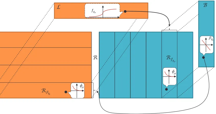
The link-binding decomposition can also be used to characterize the structure of the set of tunable regularization losses.

6.1 Equivalence Classes

A simple consequence of (37) is that the set R of tunable regularization losses φσ is the

Cartesian product of the setLof generalized logit links and the set Bof binding functions. It follows that both generalized logit links fσ and binding functions βσ define equivalence

classes inR. In fact,Rcan be partitioned according to

R=∪βσRβσ where Rβσ ={φσ|βφσ =βσ}

or

B L

EI

EI R

\I

fI

R_f I R

I

I_V V

V

V

V

V

Figure 4: The set R of tunable regularization losses can be partitioned into equivalence classes R_fφσ, isometric to the set B of binding functions, or equivalence classes Rβφσ, isometric to the set L of generalized logit links. A tunable regularization lossφσ is defined by a pair of link fφσ and binding βφσ functions.

The sets R_fσ are isomorphic to B, which is itself isomorphic to the set of continuously differentiable, monotonically decreasing, odd functions. The setsR_βσ are isomorphic toL, which is shown to be isomorphic, in Appendix B.2, to the set of parametric continuous scale probability density functions (pdfs)

ψσ(v) =

1

σψ

v

σ

, (44)

where ψ(v) has unit scale, a unique maximum at the origin, and ψ(−v) = ψ(v). The structure of the set of tunable regularization losses is illustrated in Figure 4. The set can be partitioned in two ways. The first is into a set of equivalence classesR_βσ isomorphic to the set of pdfs of (44). The second into a set of equivalence classes R_fσ isomorphic to the set of monotonically decreasing odd functions.

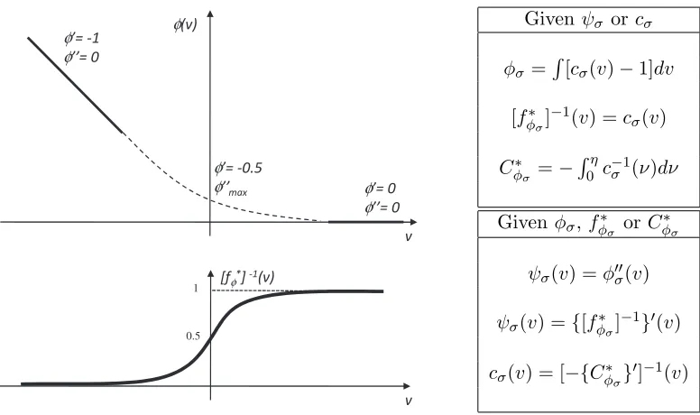
6.2 Design of Regularization Losses

An immediate consequence of the structure of R is that all tunable regularization losses can be designed by the following procedure.

1. select a scale pdfψσ(v) with the properties of (44).

2. set [f_φ∗_σ]−1(v) = cσ(v), where cσ(v) =

Rv

φ φ

φ φ φ

φ φ

1 φ

0.5

Givenψσ orcσ

φσ =R[cσ(v)−1]dv

[f_φ∗_σ]−1(v) =cσ(v) C_φ∗

σ =−

Rη

0 c

−1 σ (ν)dν

Given φσ,f_φ∗_σ orC_φ∗_σ

ψσ(v) =φ00σ(v)

ψσ(v) ={[fφ∗σ] −1_}0_(v)

cσ(v) = [−{C_φ∗_σ}0]−1(v)

Figure 5: Canonical regularization losses. Left: general properties of the loss and inverse link functions. Right: Relations between losses and scale pdfs.

3. select a binding function βφσ(v). This can be any parametric family of continuously differentiable, monotonically decreasing, odd functions.

4. define the tunable regularization loss asφ0_σ(v) = (1−[f_φ∗

σ]

−1_(v))β0

φσ(v).

5. restrictσ according to (30).

Note that the derivativeφ0_σ(v) is sufficient to implement the BoostLR algorithm. If desired, it can be integrated to produce a formula for the loss φσ(v). This defines the loss up to

a constant, which can be determined by imposing the constraint that limv→∞φσ(v) = 0.

As discussed in the previous section, this procedure enables the independent control of the regularization strength and robustness of the losses φσ(v). In fact, it follows from step 2.

and (14) that

ρφσ(v) = 1

ψσ(v)

, (45)

i.e. the choice of pdf ψσ(v) determines the regularization strength ofφσ(v). The choice of

binding function in step 3. then limits φσ(v) to an equivalence class Rβσ of regularization losses with common robustness properties. We next consider some important equivalence classes.

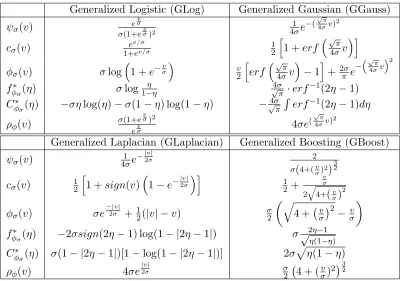
6.3 Canonical Regularization Losses

We start by considering the set of tunable regularization losses with linear binding function

Generalized Logistic (GLog) Generalized Gaussian (GGauss)

ψσ(v) e

v σ

σ(1+evσ₎2

1 4σe

−(

√

π

4σv)

2

cσ(v) e

v/σ

1+ev/σ

1 2

h

1 +erf

√

π 4σv

i

φσ(v) σlog

1 +e−vσ

v 2 h erf √ π 4σv

−1i+2σ_π e−

√ π

4σv 2

f_φ∗

σ(η) σlog

η 1−η

4σ

√

π ·erf

−1_(2η−1) C_φ∗_σ(η) −σηlog(η)−σ(1−η) log(1−η) −√4σ

π

R

erf−1(2η−1)dη ρφ(v) σ(1+e

v σ)2

evσ 4σe

(

√

π

4σv)

2

Generalized Laplacian (GLaplacian) Generalized Boosting (GBoost)

ψσ(v) _4σ1 e−

|v|

2σ 2

σ(4+(_σv)2₎32

cσ(v) 1₂

h

1 +sign(v)1−e−|2vσ|

i 1 2+ v σ 2 q

4+(v σ)

2

φσ(v) σe

−|v|

2σ + 1

2(|v| −v)

σ 2

q

4 + _σv2−_σv

f_φ∗

σ(η) −2σsign(2η−1) log(1− |2η−1|) σ

2η−1 √

η(1−η) C_φ∗_σ(η) σ(1− |2η−1|)[1−log(1− |2η−1|)] 2σpη(1−η)

ρφ(v) 4σe

|v|

2σ σ

2 4 + ( v σ)2

3₂

Table 2: Canonical tunable regularization losses

From (37), these losses are uniquely determined by their link function

φ_σ0 (v) =−(1−[f_φ∗_σ]−1(v)). (47) Their properties are discussed in Appendix D.2. As illustrated in Figure 5, they are convex, monotonically decreasing, linear (with slope −1) for large negative v, constant for large positive v, and have slope −.5 and maximum curvature at the origin. The only degrees of freedom are in the vicinity of the origin, and determine the loss margin, sinceµφσ =

1 2φ00

σ(0). Furthermore, because these losses have regularization strength ρφσ(0) =

1 φ00

σ(0), they are direct regularizers of probability scores, and regularization losses wheneverφ00_σ(0)≤1. This is reminiscent of a well known result (Bartlett et al., 2006) that Bayes consistency holds for a convex φ(v) if and only if φ0(0) ≤0. From Property 4. of Lemma 13, this holds for all regularization losses with the form of (47). The constraint φ00_σ(0) ≤1 is also equivalent to

φ00₍₀₎

σ ≤1. This is the condition of (30) for the losses of (47).

When (46) holds, it follows from (34) that f_φ∗(η) =−[C_φ∗]0(η).Buja et al. showed that the empirical risk of (4) is convex whenφis a proper loss and this relationship holds . They denoted as canonical risks the risks of (7) for which this is the case (Buja et al., 2006). For consistency, we denote the associatedφ(v) a canonical loss. This is summarized by the following definition.

We note, however, that what makes canonical losses special is not the guarantee of a convex risk, but that they have the simplest binding function with this guarantee. From Property 2. of Lemma 13, loss convexity does not require a linear binding function. On the other hand, since 1) any risk of convex loss is convex, 2) (57) holds for the linear binding function, and 3) binding functions are monotonically decreasing, the linear binding function is the simplest that guarantees a convex risk.

It should also be noted that the equivalence class of (46) includes many regularization losses. The relations of Figure 5, wherecσ(v) is the cumulative distribution function (cdf)

of the pdf ψσ(v) of (44), can be used to derive losses from pdfs or pdfs from losses. Some

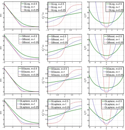
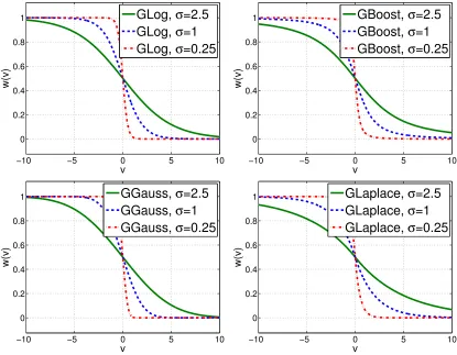
example tunable canonical regularization losses are presented in Table 2. The generalized logistic (GLog), Gaussian (GGauss), and Laplacian (GLaplacian) losses are tunable losses derived from the logistic, Gaussian, and Laplace pdfs respectively. The GBoost loss illus-trates some interesting alternative possibilities for this loss design procedure. In this case, we did not start from the pdfψσ(v) but from the minimum risk of boosting (see Table 1).

We then used the top equations of Figure 5 to derive the cdf cσ(v) and the bottom

equa-tions to obtain φσ(v) andfφ∗σ(η). The resulting pdf ψσ(v) is a special case of the Pearson type VII distribution with zero location parameter, shape parameter 3₂ and scale parameter 2σ. These losses, their optimal inverse links, and regularization strength are plotted in Fig-ure 6, which also shows how the regularization gain σ influences the loss around the origin, both in terms of its margin properties and regularization strength. Note that, due to (45), canonical losses implement all regularization behaviors possible for tunable regularization losses. This again justifies the denomination of “canonical regularization losses,” although such an interpretation does not appear to have been intended by Buja et al.

The combination of BoostLR with a canonical loss is denoted a canonical BoostLR algorithm. For a proper lossφσ,G(t)(x) converges asymptotically to the optimal predictor p∗_σ(x) =f_φ∗

σ(η(x)) and the weight function of (40) to

w∗(xi) =

1−η(xi) ifyi = 1 η(xi) ifyi =−1.

Hence, the weights of canonical BoostLR converge to the posterior example probabilities. Figure 7 shows the weight functions of the losses of Table 2. An increase in regularization gain σ simultaneously 1) extends the region of non-zero weight away from the boundary, and 2) reduces the derivative amplitude, increasing regularization strength. Hence, larger gains increase both the classification margin and the regularization of probability estimates.

6.4 Shrinkage Losses

Definition 7 A tunable regularization loss φσ(v) such that

β_φ0_σ(v) =β_φ0

v

σ

, (48)

for some βφ(v)∈ B is a shrinkage loss.

−10 −5 0 5 10 0 2 4 6 8 10 v φ (v)

GLog, σ=2.5 GLog, σ=1 GLog, σ=0.25

−1.5 −1 −0.5 0 0.5 1

0 0.2 0.4 0.6 0.8 1 v [f

*]φ

−1

(v)

GLog, σ=2.5 GLog, σ=1 GLog, σ=0.25

−6 −4 −2 0 2 4 6

0 10 20 30 40 50 v ρφ (v) GLog, σ=2.5 GLog, σ=1 GLog, σ=0.25

−10 −5 0 5 10

0 2 4 6 8 10 v φ (v)

GBoost, σ=2.5 GBoost, σ=1 GBoost, σ=0.25

−2 −1 0 1 2 0 0.2 0.4 0.6 0.8 1 v [f

*]φ

−1(v)

GBoost, σ=2.5

GBoost, σ=1

GBoost, σ=0.25

−6 −4 −2 0 2 4 6 0 10 20 30 40 50 v ρφ (v) GBoost, σ=2.5 GBoost, σ=1 GBoost, σ=0.25

−10 −5 0 5 10

0 2 4 6 8 10 v φ (v)

GGauss, σ=2.5 GGauss, σ=1 GGauss, σ=0.25

−1 −0.5 0 0.5 1

0 0.2 0.4 0.6 0.8 1 v [f

*]φ

−1

(v)

GGauss, σ=2.5 GGauss, σ=1 GGauss, σ=0.25

−6 −4 −2 0 2 4 6

0 10 20 30 40 50 v ρφ (v)

GGauss, σ=2.5

GGauss, σ=1

GGauss, σ=0.25

−10 −5 0 5 10

0 2 4 6 8 10 v φ (v)

GLaplace, σ=2.5

GLaplace, σ=1

GLaplace, σ=0.25

−2 −1 0 1 2

0 0.2 0.4 0.6 0.8 1 v [f

*]φ

−1

(v)

GLaplace, σ=2.5

GLaplace, σ=1

GLaplace, σ=0.25

−6 −4 −2 0 2 4 6

0 10 20 30 40 50 v ρφ (v) GLaplace, σ=2.5 GLaplace, σ=1 GLaplace, σ=0.25

−10 −5 0 5 10 0

0.2 0.4 0.6 0.8 1

v

w(v)

GLog, σ=2.5

GLog, σ=1

GLog, σ=0.25

−10 −5 0 5 10

0 0.2 0.4 0.6 0.8 1

v

w(v)

GBoost, σ=2.5

GBoost, σ=1

GBoost, σ=0.25

−10 −5 0 5 10

0 0.2 0.4 0.6 0.8 1

v

w(v)

GGauss, σ=2.5

GGauss, σ=1

GGauss, σ=0.25

−10 −5 0 5 10

0 0.2 0.4 0.6 0.8 1

v

w(v)

GLaplace, σ=2.5

GLaplace, σ=1

GLaplace, σ=0.25

Figure 7: BoostLR weights for various parametric regularization losses and gains. GLog (top left), GBoost (top right), GGauss (bottom left) and GLaplace (bottom right).

and (33) leads toφ0_σ(v) =φ0(v/σ). Hence,φσ is a shrinkage loss if and only if

φσ(v) =σφ

v

σ

. (49)

This enables the generalization of any proper loss of generalized logit link into a shrinkage loss. For example, using Table 1, it is possible to derive the shrinkage losses generated by the logistic

φσ(v) =σlog(1 +e−

v σ)

and the exponential loss

φσ(v) =σe−

v σ.

of (39) into

G(t)(x) =G(t−1)(x) +λg(t)(x), (50) where 0< λ <1 is a learning rate. Shrinkage is inspired by parameter regularization meth-ods from the least-squares regression literature, where similar modifications follow from the adoption of Bayesian models with priors that encourage sparse regression coefficients. This interpretation does not extend to classification, barring the assumption of the least-squares loss and some approximations (Hastie et al., 2001). In any case, it has been repeatedly shown that small learning rates (λ≤0.1) can significantly improve the generalization abil-ity of the learned classifiers. Hence, despite its tenuous theoretical justification, shrinkage is a commonly used regularization procedure.

Shrinkage losses, and the proposed view of margin losses as regularizers of probabil-ity estimates, provide a much simpler and more principled justification for the shrinkage procedure. It suffices to note that the combination of (49) and (41) leads to

w(t)_σ (xi) = −φ0σ(γi) =−φ0

γ_i

σ

= −1−[f_φ∗]−1γi

σ

β_φ0 γi σ

,

whereγi=yiG(t−1)(xi). Letting λ= 1/σ, this is equivalent to wλ(xi) =− 1−[fφ∗]−1(yiλG(xi))

β_φ0 (yiλG(xi)).

Hence, the weight function of BoostLR with shrinkage lossφσ and predictor G(x) is

equiv-alent to the weight function of standard GradientBoost with loss φand shrinked predictor 1/σG(x). Since the only other effect of replacing (39) with (50) is to rescale the final predic-torG(T)_{(x), the decision ruleh(x) produced by the two algorithms is identical. In summary,}

GradientBoost with shrinkage and a small learning rate λ is equivalent to BoostLR with a shrinkage loss of large regularization strength (1/λ). This justifies the denomination of “shrinkage losses” for the class of regularization losses with the property of (48).

It should be noted, however, that while rescaling the predictor does not affect the decision rule, it affects the recovery of posterior probabilities from the shrinked predictor. The regularization view of shrinkage makes it clear that the probabilities can be recovered with

ˆ

η(x) = [f_φ∗_σ]−1

G(T)(x)

= [f_φ∗]−1

λG(T)(x)

. (51)

−10 −8 −6 −4 −2 0 2 4 0

0.5 1 1.5 2 2.5 3 3.5 4

γ

w σ

(

γ

)

α=0 (Log)

α=0.1

α=0.2

α=0.3

α=0.4

α=0.5 (Exp)

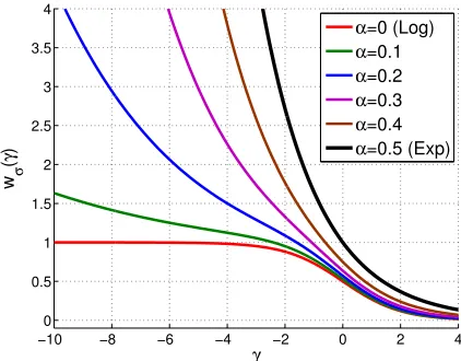
Figure 8: Weight function of theα-tunable regularization loss, for different values ofα.

6.5 α-tunable Regularization Losses

From (48), the key to the equivalence between loss-based regularization and shrinkage is the identical parameterization of [f_φ∗

σ]

−1_{(v) and β}0

φσ(v) in (33) and (48). When this is not the case, BoostLR weights are given by

wσ(xi) = − 1−[fφ∗σ] −1_(γ

i)

β_φ0_σ(γi)

= − 1−[f_φ∗]−1(λγi)

β_φ0_σ(γi)

6

= − 1−[f_φ∗]−1(λγi)

β_φ0(λγi)),

and the shrinkage interpretation no longer holds. One such loss class is defined as follows.

Definition 8 A tunable regularization loss φσ(v) such that

β_φ0_σ(v) =g(α)β0_φ

αv σ

,

where βφ(v)∈ B, g(α) is a constant that depends on α, and α≥0 is denoted α-tunable.

The additional α parameter enables α-tunable losses to independently control the link and binding functions. In fact, they generalize the previous two loss classes, reducing to shrinkage losses whenα= 1 andg(1) = 1 and canonical losses whenα= 0 andg(0)β0_φ(0) = 1. More generally, the α parameter allows the “interpolation” between pairs of canonical or shrinkage losses of equal generalized logit link. For example, the logistic and exponential losses have the scaled logit of (28) as link function, with a = 1 and a = 1₂, respectively. Since these can be written as a = _ξ+11 , for ξ = 0 and ξ = 1, scaled logits with ξ ∈ [0,1] interpolate between the links of the two losses. Similarly, the binding functions of the two losses, given by (42) and (43), are special cases of

β_φ0(v) =− 1 2−b(e

withb= 0 andb= 1. Hence, binding functions withb=ξandξ∈[0,1] interpolate between the binding functions of the two losses. It follows that

φ0(v) =− 1− e (ξ+1)v

1 +e(ξ+1)v

!

1 2−ξ(e

−ξv_+eξv_{), ξ∈[0,1]}

interpolates between the derivative of the logistic (ξ = 0) and exponential (ξ = 1) losses. The derivative of the tunable regularization loss that it generates is

φ0_µ(v) =− 1− e (ξ+1)v_µ

1 +e(ξ+1)vµ

!

1 2−ξ(e

−ξv_µ

+eξvµ_{), ξ} ∈_[0,1].

Definingσ = _ξ+1µ and α= _1+ξξ , this can be written as

φ0_σ(v) =− 1− e v σ

1 +evσ

!

1−α

2−3α(e

−αv σ +eα

v

σ), α∈

0,1

2

, (53)

i.e. a α-tunable loss of scaled logit link, g(α) = ₂1₋−_3αα, and the binding function of (52). Figure 8 shows the weight function,wσ(γ) =−φ0σ(γ),of this loss as a function of the

normal-ized marginγ =v/σ, for different values ofα. Asα varies, the weight function interpolates between the asymptotically constant weights of LogitBoost (less outlier sensitivity) and the exponential weights of AdaBoost (more sensitive to outliers).

Note that, due to their ability to independently control the link and binding functions,

α-tunable losses can always implement this type of interpolation. This can be used to design losses that adapt to the presence of outliers in the data, by cross-validation of α. It should be noted, however, that not all values ofα ≥0 lead to sensible loss functions. This is due to the fact that (49) does not hold for these losses. For shrinkage losses, where the property holds,φσ(v)→0 asv→ ∞(wheneverφ(v) has this property), guaranteeing that examples

of large positive margin have zero weight. For α-tunable losses, where (49) does not hold,

β_φ0

σ(v) can decrease to −∞ faster than 1−[f ∗

φσ]

−1_{(v) goes to zero, as v → ∞. In this}

case, examples of large positive margin can receive large positive weight, which is usually undesirable. The losses of (53) have this behavior forα >1/2.

7. Experiments

In this section we discuss various experiments conducted to evaluate different properties of probability regularization.

7.1 Experiments on Two Gaussian Classes

Vasconcelos, 2011; Rasolzadeh et al., 2006; Wu et al., 2004). We started by investigating how the probability estimates varied with the regularization gain σ. The accuracy of the probability estimates was measured by the mean squared error

M SE= 1

n n

X

i−1

[η(xi)−ηˆ(xi)]2, (54)

where η(xi) and ˆη(xi) are the true and estimated posterior probability for test example xi. The latter was obtained with (51), whereG(T)(x) is the predictor learned by BoostLR.

Three regimes were considered. The very small sample regime, where the training set containedN = 5 examples per class, the moderate sample size regime, where N = 40 and the large sample regime, where N = 1,000. Classifiers were learned with BoostLR under the three regimes, for a range of values of σ in the interval [0.5,1000]. Figure 9 shows two complementary views of the MSE data. The top row presents the classical curves of MSE vs. number of boosting iterations T, for different regularization gains. These plots are most useful to assess overfitting, which happens when there is a range ofT over which the MSE increases. It is clear that, for both the small and moderate sample sizes, all classifiers eventually overfit as the number of boosting iterations increases, while no overfitting is observed for large sample sizes. The bottom row is most useful to assess the impact of predictor regularization. The data is the same, but these plots show the evolution of the MSE withσ for fixedT. In this case, overfitting occurs on the left of each plot (small values of σ, not enough regularization) and underfitting (too much regularization) on the right.

Overall, the plots demonstrate the complementarity between loss-based probability reg-ularization and classic parameter regreg-ularization (due to early stopping, i.e. limiting the number of weak learners in the final ensemble). This is most clear in the moderate sample regime, where many of the curves of the middle column of Figure 9 (top) have the same minimum. Varying the gain σ shifts this minimum, i.e. makes it occur at different num-bers of boosting iterations. Hence, when a regularization loss is used, there is less need for early stopping (parameter regularization). This explains the empirical observation that boosted classifiers can do well even with little parameter regularization (e.g. boosted object detectors with thousands of weak learners commonly used in computer vision (Viola and Jones, 2004)). The problem with early stopping is that it can be insufficient for small sam-ples. This is visible in the left column of Figure 9 (top), where there is too little data and boosting overfitseven in the earliest iterations. The same happens for the moderate sample size (middle column of Figure 9 top) when the regularization gain is small. In these cases, by amplifying parameter based regularization, loss-based regularization can substantially improve the quality of probability estimates. For example, largerσ lead to significant gains in estimation accuracy, for all numbers of boosting iterations, in the left column of Figure 9 (bottom). Asσ increases, the best early-stopped MSE (T = 2) decreases from roughly 20% to about 5%. Hence, for small samples, loss-based regularization is much more effective than early stopping.

100 102 104 0.05 0.1 0.15 0.2 0.25 Boosting Iterations MSE 0.5 1.4 3.3 12.5 25 111.1 200 1000 100 102 104 0.025 0.03 0.035 0.04 0.045 0.05 0.055 Boosting Iterations MSE 0.5 1.4 3.3 12.5 25 111.1 200 1000 100 102 104 0 0.01 0.02 0.03 0.04 0.05 0.06 Boosting Iterations MSE 0.5 1.4 3.3 12.5 25 111.1 200 1000

0.1 1 10 100 1000

0.05 0.1 0.15 0.2 0.25 σ MSE T=2 T=5 T=10 T=20 T=30 T=75 T=100 T=500 T=2000

0.1 1 10 100 1000 0.025 0.03 0.035 .04 0.045 0.05 0.055 σ MSE T=2 T=5 T=10 T=20 T=30 T=75 T=100 T=500 T=2000

0.1 1 10 100 1000 0 0.01 0.02 0.03 0.04 0.05 0.06 σ MSE T=2 T=5 T=10 T=20 T=30 T=75 T=100 T=500 T=2000

Figure 9: Top: MSE as a function of the number of boosting iterations T for different regularization gains. Bottom: MSE as a function of regularization gain σ for different numbers of boosting iterations T. From left to right: small, moderate sized, and large samples.

100 101 102 103 100

101 102 103

Train Set Size

σ

row of Figure 9, when the number of iterationsT is fixed, the best performing regularization gain decreases with the sample size. This suggests that, whenT is fixed, the cross-validated

σ can be seen as a diagnostic of whether the classifier would benefit from the collection of further training data. Small samples (left of the figure) require large σ, while a smallσ is sufficient for large samples (right). This effect is illustrated in Figure 10, which presents a plot of the cross-validated regularization gain as a function of training set size. Note the monotonic relation between the two variables, suggesting that regularization gain can be used as a diagnostic for data scarcity. While a large σ suggests that it is worth collecting more training data, a small σ indicates that such an effort is likely not justified. This can help learning practitioners perform cost-benefit analysis of their data collection efforts.

7.2 The Role of the Link Function

The next set of experiments used ten binary UCI data sets of relatively small size: (#1) sonar, (#2) breast cancer prognostic, (#3) breast cancer diagnostic, (#4) original Wisconsin breast cancer, (#5) Cleveland heart disease, (#6) tic-tac-toe, (#7) echo-cardiogram, (#8) Haberman’s survival, (#9) Pima-diabetes, and (#10) liver disorder. These experiments aimed to evaluate the impact of of the choice of regularization (link) function on calibration and classification accuracy. Since, as discussed in Section 6.3, canonical losses implement all regularization behaviors possible for tunable regularization losses, we only considered the losses of Table 2 in these experiments. Each data set was split into five folds, four of which were used for training and one for testing. This created four train-test pairs per data set, over which the results were averaged. In all experiments, three of the four training folds were used for classifier training and one as validation set for parameter selection.

BoostLR was run for 50 iterations, using histogram-based weak learners and regular-ization gains σ ∈ [0.3,500]. Classification accuracy was measured with test error. Since the true posterior probabilities are not known for the UCI data sets, calibration cannot be evaluated with (54). A measure of calibration commonly used when this is the case is the cross-entropy between the distributions of the true η and estimated posterior probabilities ˆ

η (Niculescu-Mizil and Caruana, 2005). Assuming the quantization of all probabilities into

K probability bins, this is defined as

H(η,ηˆ) =− K

X

k=1

p(η=k) logp(ˆη =k) =−Eη[logp(ˆη)].

For large samples, the cross-entropy can be estimated with

H(η,ηˆ) =− N

X

i=1

1

N logp(ˆη(xi)).

This measure is largest for poorly calibrated classifiers that produce bimodally distributed posterior estimates, concentrated around ˆη = 0 and ˆη= 1, and smallest for well calibrated classifiers whose distribution of posteriors is less concentrated, and spread more evenly between zero and one (Niculescu-Mizil and Caruana, 2005; Mease and Wyner, 2008).

.3 .4 .5 .6 .7 .8 .9 1 2 3 4 5 6 7 8 9 10 6.5

7 7.5 8 8.5 9 9.5 10 10.5 11 11.5

σ

Avg. Rank

.3 .4 .5 .6 .7 .8 .9 1 2 3 4 5 6 7 8 9 10 5

6 7 8 9 10 11 12 13 14 15

σ

Avg. Rank

Figure 11: Average calibration (left) and classification (right) rank as a function of regu-larization gain for the GLog loss on the UCI data.

of Table 2. To produce these plots, a predictor was trained per data set, for 17 values of

σ ∈ [0.3,10]. The results were then ranked, and rank 1 (17) assigned to the value of σ

of smallest (largest) cross-entropy or classification error. The ranks of each σ were then averaged over the ten data sets (Demˇsar, 2006). Note that the curves of classification ac-curacy and cross entropy rank have similar shape, although the rank curve is smoother for cross-entropy. This is because the classifier produces binary decisions by thresholding the predictor output. Nevertheless, the two plots support the conclusion that the best values of

σ for these data sets are in the range of 4≤σ≤6. Note that the average calibration rank for this range (between 6.5 and 7.5), is substantially better than that (more than 9.5) of the logistic loss of Figure 1 (which is identical to GLog withσ = 1). For classification, the difference is similar (between 5.5 and 6.5 for 4≤σ ≤6, around 9 for σ = 1). In summary, regularization strength can have a significant impact in both classification and calibration performance. The fact that best results occur for relatively large regularization gains is not surprising, given that these data sets are relatively small.

We next attempted to quantify the intrinsic regularization gain of each data set, i.e. the regularization gain that leads to best performance on that data set across all losses, and the benefits of using that regularization over the standard values (e.g. σ = 1 for the logistic loss in LogitBoost). For this, we averaged the performance of all BoostLR classifiers learned with the four losses of Table 2, for each value ofσ and data set. We then determined the gain σopt of smallest average classification error per data set. This can be seen as a

loss-independent measure of the intrinsic regularization gain of the data set. The associated classification error is a loss-independent estimate of the performance of a classifier tuned to this intrinsic regularization value. These results are summarized in Table 3 (top). For comparison, we also present the results of AdaBoost, LogitBoost (GLog loss with σ = 1), the average performance of BoostLR with the four losses of Table 2 when the bandwidth is constrained toσ = 1, and the drop in classification error due to the tuning to the intrinsic regularization gain of the data set. To compute this drop, we defined as 1 the average