Undercomplete Blind Subspace Deconvolution

Undercomplete Blind Subspace Deconvolution

Zolt´an Szab´o [email protected]

Barnab´as P´oczos [email protected]

Andr´as L˝orincz [email protected]

Department of Information Systems E¨otv¨os Lor´and University

P´azm´any P. s´et´any 1/C Budapest H-1117, Hungary

Editor: Michael Jordan

Abstract

We introduce the blind subspace deconvolution (BSSD) problem, which is the extension of both the blind source deconvolution (BSD) and the independent subspace analysis (ISA) tasks. We examine the case of the undercomplete BSSD (uBSSD). Applying temporal concatenation we reduce this problem to ISA. The associated ‘high dimensional’ ISA problem can be handled by a recent tech-nique called joint f-decorrelation (JFD). Similar decorrelation methods have been used previously for kernel independent component analysis (kernel-ICA). More precisely, the kernel canonical cor-relation (KCCA) technique is a member of this family, and, as is shown in this paper, the kernel generalized variance (KGV) method can also be seen as a decorrelation method in the feature space. These kernel based algorithms will be adapted to the ISA task. In the numerical examples, we (i) examine how efficiently the emerging higher dimensional ISA tasks can be tackled, and (ii) explore the working and advantages of the derived kernel-ISA methods.

Keywords: undercomplete blind subspace deconvolution, independent subspace analysis, joint decorrelation, kernel methods

1. Introduction

Independent component analysis (ICA) (Jutten and Herault, 1991; Comon, 1994) aims to recover linearly or non-linearly mixed independent and hidden sources. There is a broad range of tions for ICA, such as blind source separation, feature extraction and denoising. Particular applica-tions include the analysis of financial and neurobiological data, fMRI, EEG, and MEG. For recent review concerning ICA the reader is referred to the literature (Hyv¨arinen et al., 2001; Cichocki and Amari, 2002).

Traditional ICA algorithms are one-dimensional in the sense that all sources are assumed to be independent real valued random variables. Nonetheless, applications in which only certain groups of sources are independent may be highly relevant in practice. In this case, the independent sources can be multidimensional. For instance, consider the generalization of the cocktail-party problem, where independent groups of people are talking about independent topics or more than one group

of musicians is playing at the party. The separation task requires an extension of ICA, which can

Strenuous efforts have been made to develop ISA algorithms (Cardoso, 1998; Akaho et al., 1999; Hyv¨arinen and Hoyer, 2000; Hyv¨arinen and K ¨oster, 2006; Vollgraf and Obermayer, 2001; Bach and Jordan, 2003; St ¨ogbauer et al., 2004; P ´oczos and L ˝orincz, 2005b,a; Theis, 2005a,b, 2006; Szab ´o and L˝orincz, 2006; Nolte et al., 2006). For the most part, ISA-related theoretical problems concern the estimation of entropy or of mutual information. For this, the k-nearest neighbors (P ´oczos and L˝orincz, 2005b) and the geodesic spanning tree methods (P ´oczos and L ˝orincz, 2005a) can be ap-plied. Other recent approaches seek independent subspaces via kernel methods (Bach and Jordan, 2003) and joint block diagonalization (Theis, 2005a, 2006).

Another extension of the original ICA task is the blind source deconvolution (BSD) problem. Such a problem emerges, for example, at a cocktail-party being held in an echoic room. Several BSD algorithms were developed in the past. See, for example, the review of Pedersen et al. (2007). Like ICA, BSD has several applications: (i) remote sensing applications; passive radar/sonar process-ing (MacDonald and Cain, 2005; Hedgepeth et al., 1999), (ii) image-deblurrprocess-ing, image restoration (Vural and Sethares, 2006), (iii) speech enhancement using microphone arrays, acoustics (Douglas et al., 2005; Mitianoudis and Davies, 2003; Roan et al., 2003; Araki et al., 2003), (iv) multi-antenna wireless communications, sensor networks (Akyildiz et al., 2002; Deligianni et al., 2006), (v) biomedical signal—EEG, ECG, MEG, fMRI—analysis (Jung et al., 2000; Glover, 1999; Dyrholm et al., 2007), (vi) optics (Kotzer et al., 1998), (vii) seismic exploration (Karslı, 2006).

The simultaneous assumption of the two extensions, that is, ISA combined with BSD, seems to be a more realistic model than either of the two models alone. For example, at the cocktail-party, groups of people or groups of musicians may form independent source groups and echoes could be present. This task will be called blind subspace deconvolution (BSSD). We treat the undercomplete case (uBSSD) here. In terms of the cocktail-party problem, it is assumed that there are more microphones than acoustic sources. Here we note that the complete, and in particular the overcomplete, BSSD task is challenging and as of yet no general solution is known. We can show that temporal concatenation turns the uBSSD task into an ISA problem. One of the most stringent applications of BSSD could be the analysis of EEG or fMRI signals. The ICA assumptions could be highly problematic here, because some sources may depend one another, so an ISA model seems better. Furthermore, the passing of information from one area to another and the related delayed and transformed activities may be modeled as echoes. Thus, one can argue that BSSD may fit this important problem domain better than ICA or even ISA.

In principle, the ISA problem can be treated with the methods listed above. However, the dimension of the ISA problem derived from an uBSSD task is not amenable to state-of-the-art ISA methods. According to a recent decomposition principle, the ISA Separation Theorem (Szab ´o et al., 2006b), the ISA task can be divided into two consecutive steps under certain conditions: after the application of the ICA algorithm, the ICA elements need to be grouped.1 The importance of this direction stems from the fact that ICA methods can deal with problems in high dimensions. The derived ISA task will be solved with the use of the decomposition principle augmented by the joint f-decorrelation (JFD) technique (Szab ´o and L˝orincz, 2006).

larly to the JFD and the KCCA methods, the KGV technique deals with nonlinear decorrelation in function spaces. We found that they can be more precise but are limited to smaller problems.

The paper is structured as follows: Section 2 formulates the problem domain. Section 3 shows how to transform the uBSSD task into an ISA task. The JFD method, which we use to solve the derived ISA task, is the subject of Section 4. This section also addresses how to tailor the KCCA and KGV kernel-ICA methods to solve the ISA problem. Section 5 contains the numerical illustrations and conclusions are drawn in Section 6.

2. The BSSD and the ISA Model

The BSSD task and its special case, the ISA model, are defined in Section 2.1. Section 2.2 details the ambiguities of the ISA task. Section 2.3 introduces some possible ISA cost functions.

2.1 The BSSD Equations

Here, we define the BSSD task. Assume that we have M hidden, independent, multidimensional

components (random variables). Suppose also that only their casual FIR filtered mixture is available

for observation:2

x(t) =

L

∑

Hls(t−l), (1)

where s(t) =s1(t);. . .; sM(t)∈RMd is a vector concatenated of components sm(t)∈Rd. For a given m, sm(t)is i.i.d. (independent and identically distributed) in time t, sms are non-Gaussian, and

I(s1, . . . ,sM) =0, where I stands for the mutual information of the arguments. The total dimension of the components is Ds:=Md, the dimension of the observation x is Dx. Matrices Hl ∈_RDx×Ds (l=0, . . . ,L) describe the mixing, these are the mixing matrices. Without any loss of generality it may be assumed that E[s] =0, where E denotes the expectation value. Then E[x] =0 holds, as well. The goal of the BSSD problem is to estimate the original source s(t)by using observations x(t)only.

The case L=0 corresponds to the ISA task, and if d =1 also holds then the ICA task is recovered. In the BSD task d=1 and L is a non-negative integer. Dx>Ds is the undercomplete,

Dx=Ds is the complete, and Dx<Dsis the overcomplete task. Here, we treat the undercomplete BSSD (uBSSD) problem. We will transform the uBSSD task to undercomplete ISA (uISA) or to complete ISA. From now on they both will be called ISA.

Note 1 Mixing matrices Hl (0≤ l ≤ L) have a one-to-one mapping to polynomial matrix3

H[z]:=∑L_l=0Hlz−l ∈R[z]Dx×Ds_{, where z is the time-shift operation, that is (z}−1_{u)(t) =u(t−1).}

H[z]may be regarded as an operation that maps Ds-dimensional series to Dx-dimensional series.

Equation (1) can be written as x=H[z]s.

Note 2 It can be shown (Rajagopal and Potter, 2003) that in the uBSSD task H[z]has a polynomial matrix left inverse W[z]∈_R[z]Dx×Ds _{with probability 1, under mild conditions. In other words, for} these polynomial matrices W[z]and H[z], W[z]H[z]is the identity mapping. The mild condition is as follows: Coefficients of polynomial matrix H[z], that is, random matrix[H0;. . .; HL]is drawn from

a continuous distribution. Under this condition, hidden source s(t) can be estimated by a suitable causal FIR filtered form of observation x(t).

For the uBSSD task it is assumed that H[z]has a polynomial matrix left inverse. For the uISA and ISA tasks it is supposed that mixing matrix H0∈RDx×Ds_{has full column rank, that is its rank is} Ds.

2.2 Ambiguities of the ISA Model

Because the uBSSD task will be reduced to ISA, it is important to see the ambiguities of the ISA task. First, the complete ISA problem (L=0,Dx=Ds) is presented, the undercomplete ISA will be treated later.

The identification of the ISA model is ambiguous. However, the ambiguities are simple (Theis, 2004): hidden multidimensional components can be determined up to permutation and up to in-vertible transformation within the subspaces. Ambiguities within the subspaces can be weakened. Namely, because of the invertibility of mixing matrix H[z] =H0∈RDs×Ds_{, it can be assumed}

with-out any loss of generality that both the sources and the observation are white, that is,

E[s] =0,cov[s] =IDs, E[x] =0,cov[x] =IDx,

where IDs is the Ds-dimensional identity matrix and cov is the covariance matrix. It then follows

that the mixing matrix H0and thus the demixing matrix W=H−1₀ are orthogonal: IDs =cov[x] =E[xx

∗_{] =H0E[ss}∗_]H∗

0=H0IDsH

∗

0=H0H∗0,

where∗denotes transposition. In sum, H0,W∈ODs_{, whereO}Ds _{denotes the set of Ds-dimensional}

orthogonal matrices. Now, smsources are determined up to permutation and orthogonal transforma-tion.

In order to transform the undercomplete ISA task into a complete ISA task with white observa-tions let C :=cov[x] =E[xx∗] =H0H∗0∈RDx×Dx denote the covariance matrix of the observation. Rank of C is Ds, since the rank of matrix H0 is Ds according to our assumptions. Matrix C is symmetric (C=C∗), thus it can be decomposed as follows: C=UDU∗, where U∈RDx×Ds_{, and}

the columns of matrix U are orthogonal, that is, U∗U=IDs. Furthermore, the rank of diagonal

matrix D∈RDs×Ds _{is D}

s. The principal component analysis can provide a decomposition in the desired form. Let Q :=D−1/2U∗∈RDs×Dx_{. Then the original observation x can be modified to}

x0 :=Qx=QH0s∈RDs. The resulting x0 is white and can be regarded as the observation of a

complete ISA task having mixing matrix QH0∈ODs. 2.3 ISA Cost Functions

After the whitening procedure (Section 2.2), the ISA task can be viewed as the minimization of the mutual information between the estimated components on the orthogonal group:

JI(W):=I y1, . . . ,yM

, (2)

The ISA task can be rewritten into the minimization of the sum of Shannon’s multidimensional differential entropies (P ´oczos and L ˝orincz, 2005b):

JH(W):= M

∑

H(ym), (3)

where y=Wx, y=y1;. . .; yM, ym∈Rd, W∈

O

Note 3 Until now, we formulated the ISA task by means of the entropy or the mutual information of

multidimensional random variables, see Equations (2) and (3). However, any algorithm that treats mutual information between 1-dimensional random variables can also be sufficient. This statement is based on the considerations below. Well-known identities of mutual information and entropy expressions (Cover and Thomas, 1991) show that the minimization of cost function

JH,I(W):= M

∑

d

∑

H(ym_i )−

M

∑

I(ym₁, . . . ,ym_d),

or that of

JI,I(W):=I y11, . . . ,yMd

−

M

∑

I(ym₁, . . . ,ym_d)

can also solve the ISA task. Here, y=Wx is the estimated ISA source, where x∈RD is the whitened observation in the ISA model. W∈OD _{is the estimated ISA demixing matrix, and in} y=y1;. . .; yM∈RDthe ym∈Rd, m=1, . . . ,M, represent the estimated components with coordi-nates ym_i ∈R. The first term of both cost functions JH,Iand JI,Iis an ICA cost function. Thus, these

first terms can be fixed by means of ICA preprocessing.4 In this case, if the Separation Theorem holds (for details see Section 3.2), then term ∑M_m=1I(ym₁, . . . ,ym_d) implies that the maximization of the sum of mutual information between 1-dimensional random variables within the subspaces is sufficient for solving the ISA task.

3. Reduction Steps

Here we show that the direct search for inverse FIR filter can be circumvented (Note 2). Namely, temporal concatenation reduces the uBSSD task to an (u)ISA problem (Section 3.1). Our earlier results will allow further simplifications. We will reduce the ISA task to an ICA task plus a search for optimal permutation of the ICA coordinates. This decomposition principle will be elaborated in Section 3.2 by means of the Separation Theorem.

3.1 Reduction of uBSSD to (u)ISA

We reduce the uBSSD task to an ISA problem. The BSD literature provides the basis for our reduction; F´evotte and Doncarli (2003) use temporal concatenation in their work. This method can be extended to multidimensional sm_{components in a natural fashion:}

Let L0 be such that

DxL0≥Ds(L+L0) (4)

is fulfilled. Such L0exists due to the undercomplete assumption Dx>Ds:

L0≥

DsL

Dx−Ds

. (5)

This choice of L0guarantees that the reduction gives rise to an (under)complete ISA task: let xm(t) denote the mth coordinate of observation x(t)and let the matrix Hl ∈RDx×Md _{be decomposed into}

1×d sized blocks. That is, Hl = [Hi j_l ]_i=1..D

x,j=1..M (H

i j

l ∈R1×d), where i and j denote row and column indices, respectively. Using notations

Sm(t):= [sm(t); sm(t−1);. . .; sm(t−(L+L0) +1)]∈Rd(L+L0),

Xm(t):= [xm(t); xm(t−1);. . .; xm(t−L0+1)]∈RL

0

,

S(t):= [S1(t);. . .; SM(t)]∈RMd(L+L0)=Ds(L+L0),

X(t):= [X1(t);. . .; XDx_(t)]∈RDxL0_,

Ai j:=

     

Hi j₀ . . . Hi j_L 0 . . . 0 . .. . ..

. .. . .. 0 . . . 0 Hi j₀ . . . Hi j_L

     ∈R

L0×d(L+L0)_,

A := [Ai j]i=1..Dx,j=1..M∈R

DxL0×Md(L+L0)=DxL0×Ds(L+L0)_,

model

X(t) =AS(t) (6)

can be obtained. Here, sm(t)s are i.i.d. in time t, they are independent for different m values, and Equation (4) holds for L0. Thus, (6) is either an undercomplete or a complete ISA task, depending on the relation of the l.h.s and the r.h.s of (4): the task is complete if the two sides are equal. The number of the components and the dimension of the components in task (6) are M(L+L0)and d, respectively.

If we end up with an undercomplete ISA problem in (6) then it can be reduced to a complete one, as was shown in Section 2.2. Thus, choosing the minimal value for L0in (5), the dimension of the obtained ISA task is

DISA:=Ds(L+L0) =Ds

L+

DsL

Dx−Ds

. (7)

Taking into account the ambiguities of the ISA task (Section 2.2), the original smcomponents will occur L+L0 times and up to orthogonal transformations. As a result, in the ideal case, our estima-tions are as follows

ˆsm_k :=Fm_ksm∈Rd,

where k=1, . . . ,L+L0, Fm_k ∈Od_. 3.2 Reduction of ISA to ICA

ICA estimation is executed by minimizing I(y1₁, . . . ,yM_d). In the second step, the ICA elements are grouped by finding an optimal permutation. This principle will be formalized in Section 3.2.1. Section 3.2.2 provides sufficient conditions for the theorem.

3.2.1 THEISA SEPARATIONTHEOREM

We state the ISA Separation Theorem for components having possibly different dmdimensions: Theorem 1 (Separation Theorem for ISA) Let y= [y1;. . .; yD] =Wx∈RD, where W∈

O

the dm-dimensional unit sphere, that isSdm :={w∈Rdm:∑di=m1w2i =1}.

Presume that the u :=sm∈_Rdm _{sources(m=1, . . . ,M)of the ISA model satisfy condition}

H

dm

∑

wiui !

≥

dm

∑

w2_iH(ui),∀w∈Sdm, (8)

and that the ICA cost function JICA(W) =∑Di=1H(yi)has minimum over the orthogonal matrices in WICA. Then it is sufficient to search for the solution to the ISA task as a permutation of the solution of the ICA task. Using the concept of demixing matrices, it is sufficient to explore forms

WISA=PWICA,

where P∈RD×Dis a permutation matrix to be determined and WISAis the ISA demixing matrix. The proof of the theorem is presented in Appendix A. It is intriguing that if (8) is satisfied then the simple decomposition principle provides the global minimum of (2). In the literature on joint block diagonalization (JBD) Abed-Meraim and Belouchrani (2004) have put forth a similar conjecture recently. According to this conjecture, for quadratic cost function, if Jacobi optimization is applied, the block-diagonalization of the matrices can be found by the optimization of permutations follow-ing the joint diagonalization of the matrices. ISA solutions formulated within the JBD framework (Theis, 2005a,b, 2006; Szab ´o and L˝orincz, 2006) make efficient use of this idea in practice. Theis (2006) could justify this approach for local minimum points.

3.2.2 SUFFICIENTCONDITIONS OF THEISA SEPARATIONTHEOREM

The question of which types of sources satisfy the Separation Theorem is open. Equation (8) pro-vides only a sufficient condition. Below, we list sources smthat satisfy (8). Details and the extension of the Separation Theorem for complex variables can be found in a technical report of Szab ´o et al. (2006b).

1. Assume that variables u=smsatisfy the so-called w-EPI condition (EPI is shorthand for the

entropy power inequality, Cover and Thomas, 1991), that is,

e2H(∑di=1wiui)_≥

d

∑

e2H(wiui)_,∀w∈Sd_{. (9)}

2. The (9) w-EPI condition is valid

(a) for spherically symmetric or shortly spherical variables (Fang et al., 1990). The dis-tribution of such variables is invariant for orthogonal transformations.5 Sketch of the proof (u=sm): the w-EPI condition concerns projections to unit vectors. For spherical variables, the distribution and thus the entropy of these projections are independent of w∈Sd_{. Because e}2H(wiui)_=e2H(ui)_w2

i and w∈Sd, the w-EPI is satisfied with equality

∀w∈Sd.

(b) for 2-dimensional variables invariant to 90◦rotation. Under this condition, density func-tion h of component smis subject to the following invariance

h(u1,u2) =h(−u2,u1) =h(−u1,−u2) =h(u2,−u1) ∀u∈R2

.

Sketch of the proof (u=sm): Assume that function f :S2 3w7→H ∑d_i=1wiui

has global minimum on setS2∩ {w≥0}.6Let this minimum be at wm∈R2. Then, the 90◦ invariance warrants that function f take its global minimum also on w⊥_m∈R2, which is perpendicular to wm. Let (Cm)∗= [wm,w⊥_m]∈

O

A special case of this requirement is invariance to permutation and sign changes

h(±u1,±u2) =h(±u2,±u1).

In other words, there exists a function g :R2→R, which is symmetric in its variables and

h(u) =g(|u1|,|u2|). Special cases within this family are distributions

h(u) =g

∑

i

|ui|p !

(p>0),

which are constant over the spheres of Lp-space. They are called Lpspherical variables which, for p=2, corresponds to spherical variables.

(c) for certain weakly dependent variables: Takano (1995) has determined sufficient condi-tions when EPI holds.7 If the EPI property is satisfied on unit sphereSd, then the ISA Separation Theorem holds (Lemma 1).

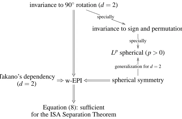
These results are summarized schematically in Table 1.

5. In the ISA task the non-degenerate affine transformations of spherical variables, the so called elliptical variables, do not provide valuable generalizations due to the ambiguities of the ISA task.

6. Relation w≥0 concerns each coordinate.

invariance to 90◦rotation (d=2)

specially S S S S S

)

)

S S S S S

invariance to sign and permutation specially

Lpspherical (p>0)

Takano’s dependency

(d=2) +3w-EPI

spherical symmetry

k

s

generalization for d=2

O

O

Equation (8): sufficient for the ISA Separation Theorem

Table 1: Sufficient conditions for the ISA Separation Theorem.

4. ISA Methods

We showed how to convert the uBSSD task to an ISA task in Section 3.1. In the following we will present methods that can solve the ISA task. In Section 4.1 we treat estimations of the mutual information of the ISA cost functions in Section 2.3. Methods that can optimize these cost functions are elaborated in Section 4.2. We also present here the pseudocode of the procedures studied. In Section 4.3 we review methods that can treat non-equal or unknown component dimensions. In what follows, and in accordance with (1), let x∈RD denote the whitened observation, while y= [y1;. . .; yM] =Wx∈RD(W∈OD) and ym∈Rd(m=1, . . . ,M)stand for the estimated source and its components in the ISA task, respectively.

4.1 Dependency Estimations

Here we introduce two dependency estimators. First, in Section 4.1.1 we describe a decorrelation method that uses a set of functions jointly. This method is called joint f-decorrelation (JFD) method (Szab´o and L˝orincz, 2006). Our second technique (Section 4.1.2) generalizes earlier kernel-ICA methods for the ISA task. The motivation for this latter method is the efficiency and precision of kernel-ICA methods in finding independent components (Bach and Jordan, 2002). Our experiences are similar with kernel-ISA methods, see Section 5.3. We found that kernel-ISA methods need more computations, but can provide more precise solutions than the JFD technique.

4.1.1 THEJFD METHOD

The JFD method estimates the hidden smcomponents through the decorrelation over a function set

for function f= [f1;. . .; fM]∈Fover t=1, . . . ,T be denoted by

Σ(f,T,W) =cov_c[f(y),f(y)] =

= 1

T

T

∑

(

f[y(t)]− 1 T

T

∑

f[y(k)]

)(

f[y(t)]−1 T

T

∑

f[y(k)]

)∗

,

Σi,j_{(f,T,W) =} c

covfi yi,fj yj=

= 1

T

T

∑

(

fi[yi(t)]−1 T

T

∑

fi[yi(k)]

)(

fj[yj(t)]−1 T

T

∑

fj[yj(k)]

)∗

.

Then, the joint decorrelation onFcan be formulated as the minimization of cost function

JJFD(W):=

∑

kN◦Σ(f,T,W)k2_F. (10)

Here: (i) W∈OD_{, (ii)Fdenotes a set ofR}D_→RD_{functions, and each function acts on each} coor-dinate separately, (iii)◦denotes the point-wise multiplication, called the Hadamard-product, (iv) N masks according to the subspaces, N :=ED−IM⊗Ed, where all elements of matrix ED∈_RD×D_and Ed∈Rd×dare equal to 1,⊗is the Kronecker-product, (v)k·k2_F denotes the square of the Frobenius norm, that is, the sum of the squares of the elements.

Cost function (10) can be interpreted as follows: for any function fm:Rd →_Rd _{that acts on} independent variables ym (m=1, . . . ,M)the variables fm(ym) remain independent. Thus, covari-ance matrixΣ(f,T,W) of variable f(y) =f1 y1;. . .; fM yM is block-diagonal. Independence of estimated sources ymis gauged by the uncorrelatedness on the function set F. Thus, the non-block-diagonal portions (Σi,j_{(f,T,W), i6= j) of covariance matricesΣ(f,T,W)are punished. This} principle is expressed by the termkN◦Σ(f,T,W)k2_F.

4.1.2 KERNEL-ISA METHODS

Two alternatives for the ISA cost function of (10) are presented. They estimate the mutual informa-tion based ISA cost defined in (2) via kernels: the KCCA and KGV kernel-ICA methods of Bach and Jordan (2002) are extended to the ISA task. The original methods estimate pair-wise indepen-dence between 1-dimensional random variables.8 The extension to the multidimensional case is straightforward, the arguments of the kernels can be modified to multidimensional variables and the derivation of Bach and Jordan (2002) can be followed. The main steps are provided below for the sake of completeness. The resulting expressions can be used for the estimation of dependence between multidimensional random variables. The performance of these simple extensions on the related ISA applications is shown in Section 5.3.2.

The KCCA Method First, the 2-variable-case is treated and then it will be generalized to many variables.

2-variable-case Assume that the mutual dependence of two random variables u∈Rd1_{and v∈R}d2

has to be measured. Let positive semi-definite kernels ku_(·,·):Rd1_×Rd1_{→R, and k}v_(·,·):Rd2_×

Rd2 _{→Rbe chosen in the respective spaces. LetF}u_andFv_{denote the reproducing kernel Hilbert}

spaces (RKHS) (Aronszajn, 1950; Wahba, 1999; Sch ¨olkopf et al., 1999) associated with the kernels. Here,FuandFvare function spaces having elements that perform mappingsRd1_→RandRd2_→R,

respectively. Then the mutual dependence between u and v can be measured, for instance, by the following expression:

J_KCCA∗ (u,v,Fu,Fv):= sup g∈Fu_,h∈Fv

corr[g(u),h(v)],

where corr denotes correlation.

The value of J_KCCA∗ can be estimated empirically: assume that we have T samples both from u and from v. These samples are u1, . . . ,uT ∈Rd1 _{and v1, . . . ,vT ∈R}d2_{. Then, using notations}

¯

g := _T1 ∑T

k=1

g(uk), ¯h :=_T1 ∑T

k=1

g(vk), the empirical estimation of J_KCCA∗ could be the following:

J_KCCA∗,emp(u,v,Fu,Fv):= sup g∈Fu_,h∈Fv

1 T∑

T

t=1[g(ut)−g¯][h(vt)−¯h] q

1 T∑

T

t=1[g(ut)−g¯]2 q

1 T∑

T

t=1[h(vt)−¯h]2

.

However, it is worth including some regularization for J_KCCA∗ (Fukumizu et al., 2007), therefore

J_KCCA∗ is modified to

JKCCA(u,v,Fu,Fv):= sup g∈Fu_,h∈Fv

cov[g(u),h(v)]

q

var[g(u)] +κkgk2Fu q

var[h(v)] +κkhk2Fv

, (11)

where expression ‘var’ stands for variance,κ>0 is the regularization parameter, k.k_F2u andk.k2_Fv

denote the RKHS norm of their arguments inFu_andFv_{, respectively. Now, expanding the} denom-inator up to second order inκ, setting the expectation value of the samples to zero in the respective RKHSs, and using the notationκ2:=κT

2 (Bach and Jordan, 2002), the empirical estimation of (11) is

ˆ

J_KCCAemp (u,v,Fu,Fv) = sup c1∈RT,c2∈RT

c∗₁Keu_Kev_c 2 r

c∗₁Keu₊κ2_I T

2 c1

r

c∗₂Kev₊κ2_I T

2 c2

, (12)

whereKeu,Kev∈RT×T are the so-called centered kernel matrices: These matrices are derived from kernel matrices Ku= [k(ui,uj)]i,j=1,...,T,Kv= [k(vi,vj)]i,j=1,...,T∈RT×T, as is described below. Let 1T∈_RT _{denote a vector whose all elements are equal to 1 and let H :=IT−}1

T1T1∗T ∈RT×Tdenote the so-called T -dimensional centering matrix. ThenKeu:=HKuH,Kev:=HKvH.

Computing the stationary points of ˆJ_KCCAemp in (12), that is, setting 0= ∂Jˆ emp

KCCA

∂c , the resulting task is to solve a generalized eigenvalue problem of the form Cξ=µDξ:

(Keu+κ2IT)2 _Keu_Kev

e

KvKeu (Kev+κ2IT)2 !

c1 c2

= (1+γ) (Ke

u₊κ2IT₎2 ₀ 0 (Kev+κ2IT)2

! c1 c2

,

Generalization for many variables The KCCA method can be generalized for more than two random variables and can be used to measure pair-wise dependence: Let us introduce the fol-lowing notations: Let y1 ∈Rd1_{, . . . ,y}M _∈RdM _{be random variables. We want to measure the}

dependence between these variables. Let positive semi-definite kernels km(·,·):Rdm_×Rdm _→R (m=1, . . . ,M)be chosen in the respective spaces. LetFm_{denote the RKHS associated with} ker-nel km(·,·). Having T samples ym₁, . . . ,ym_T for all random variables ym (m=1, . . . ,M), matrices Km:= [km(ym_i ,ym_j)]i,j=1,...,T ∈RT×T andKem:=HKmH∈RT×T can be created. Let the regular-ization parameter be chosen asκ>0 and let κ2 denote the auxiliary variableκ2:=κT

2 . It can be proven that the computation of ˆJ_KCCAemp involves the solution of the following generalized eigenvalue problem:     

(Ke1+κ2IT)2 _Ke1_Ke2 _{· · · K}e1_KeM e

K2Ke1 (Ke2+κ2IT)2 _{· · · K}e2_KeM ..

. ... ...

e

KMKe1 KeMKe2 · · · (KeM+κ2IT)2           c1 c2 .. . cM    

= (13)

=λ     

(Ke1+κ2IT)2 0 · · · 0 0 (Ke2+κ2I)2 _{· · · 0}

..

. ... ...

0 0 · · · (KeM+κ2I)2           c1 c2 .. . cM     .

Analogously to the two-variable-case, the largest eigenvalue of this task is a measure of the value of the pair-wise dependence of the random variables.

The KGV Method Equation (2) in Section 2.3 indicates that the ISA task can be seen as the minimization of the mutual information. The basic idea of the KGV technique is that—even for non-Gaussian variables—it estimates the mutual information by the Gaussian approximation (Bach and Jordan, 2002). Namely, let y= [y1;. . . ,yM]be multidimensional normal random variable with covariance matrix C. Let Ci,j_∈Rdm×dm _{denote the cross-covariance between components of y}m_∈

Rdm_{. The mutual information between components y}1_{, . . . ,y}M_{is (Cover and Thomas, 1991):} I(y1, . . . ,yM) =−1

2log

det C ∏M

m=1det Cm,m

.

The quotient _∏M det C

m=1det Cm,m is called the generalized variance. If y is not normal—this is the typical

situation in the ISA task—then let us transform the individual components ymusing feature mapping

ϕassociated with the reproducing kernel and assume that the image is a normal variable. Thus, the cost function

JKGV(W):=− 1 2log

det(

K

∏M

m=1det(

K

(14) is associated with the ISA task. In Equation (14) φ(y):= [ϕ(y1_{);. . .;ϕ(y}M_)],

K

K

m=1det(Km,m)

is called the kernel

generalized variance (KGV).

Theorem 2 Let Σ∈_RD×D _{be a positive semi-definite matrix, let Σ}m,m_∈Rdm×dm _{denote the m}th block in the diagonal of matrixΣ, and let D=∑M_m=1dm. Then the function

0≤Q(Σ):=−1

2log

det(Σ)

∏M

m=1det(Σm,m)

is 0 iffΣ=blockdiag(Σ1,1, . . . ,ΣM,M).

This theorem can be proven for dm≥1, as in the case of dm=1 (Cover and Thomas, 1991), see the work of Szab ´o and L˝orincz (2006). The theorem implies the following:

Corollary Setting Σ:=

K

K

We note that the kernel covariance (KC) ICA method (Gretton et al., 2005)—similarly to the KCCA method—can be extended to measure the mutual dependence of multidimensional random variables and thus to solve the ISA task. Again, the computation of the cost function can be con-verted to the solution of a generalized eigenvalue problem. This eigenvalue problem is provided in Appendix B for the sake of completeness.

Note 4 The KCCA, KGV and KC methods can estimate only pair-wise dependence. Nonetheless,

the joint mutual information can be estimated by recursive methods computing pair-wise mutual information: for the mutual information of random variables ym∈Rdm _{(m=1, . . . ,M) it can be} shown that the recursive relation

I(y1, . . . ,yM) =

M

∑

I ym,ym+1, . . . ,yM (15)

holds (Cover and Thomas, 1991). Thus, for example, the KCCA eigenvalue problem of (13) can be replaced by pair-wise estimation of mutual information. We note that the tree-dependent component analysis model (Bach and Jordan, 2003) estimates the joint mutual information from the pair-wise mutual information.

4.2 Optimization of ISA Costs

There are several possibilities to optimize ISA cost functions:

1. Without ICA preprocessing, optimization problems concern either the Stiefel manifold (Edel-man et al., 1998; Lippert, 1998; Plumbley, 2004; Quinquis et al., 2006) or the flag (Edel-manifold (Nishimori et al., 2006). According to our experiences, these gradient based optimization methods may be stuck in poor local minima.

Input of the algorithm

ISA observation:{x(t)}t=1,...,T Optimization9

ICA: on the whitened observation x⇒ˆsICAestimation Permutation search

P :=ID repeat

sequentially for∀p∈Gm1_,q∈Gm2_(m

16=m2): if J(PpqP)<J(P)

P :=PpqP end

until J(·)decreases in the sweep above Estimation

ˆsISA=PˆsICA

Table 2: Pseudocode of the ISA Algorithm. Cost J stands for the ISA cost function of JFD, KCCA, or KGV methods. The permutation matrix of the ISA Separation Theorem is the variable of J.

permutation search is often sufficient for the estimation of the ISA subspaces. However, it is easy to generate examples in which this is not true (P ´oczos and L ˝orincz, 2005a). In such cases, global permutation search method of higher computational burden may become neces-sary (Szab´o et al., 2006a).

4.3 Different and Unknown Component Dimensions

Here we give a quick overview how one can handle situations when the dimensions of the subspaces are unequal, unknown, or both. Note that the introduced uBSSD-ISA reduction, the ISA ambiguities (Theis, 2006) and the Separation Theorem remain the same for subspaces of different dimensions, and thus it is sufficient to consider the ISA problem.

1. If the dimensions of the subspaces are different but known, the ISA task can be solved (a) the mask N of the JFD method should be modified (see Equation 10).

(b) the kernel-ISA methods include this situation; they were introduced for different sub-space dimensions.

2. If the dimension of the hidden source s is known, but the individual dimensions of compo-nents smare not, then clustering can exploit the dependencies between the coordinates of the estimated sources. For example:

(a) If we assume that the hidden s source has block diagonal AR dynamics of the form s(t+1) = Fs(t) +e(t)—F=blockdiag F1, . . . ,FM—then connectivity of the esti-mated matrix ˆF may help (P´oczos and L ˝orincz, 2006). One may assume that the i and the j coordinates are ‘ ˆF-connected’ if value max{|Fˆi j|,|Fˆji|}is above a certain threshold. 9. LetG1_{, . . . ,G}M_{denote the indices of the 1}st_{, . . . ,M}th_{subspaces, that is,G}m_{:={(m−1)d+1, . . . ,md}, and}

(b) Similar considerations can be applied in the ISA problem, for example, by using cumu-lant based matrices (Theis, 2006).

(c) Weaknesses of the threshold based method include (i) the uncertainty in choosing the threshold, and (ii) the fact that the methods are sensitive to the threshold. More ro-bust solutions can be designed if the dependencies, for example, the mutual information amongst the coordinates, are used to construct an adjacency matrix and apply a cluster-ing method for this matrix. One might use, for example, hierarchical (St ¨ogbauer et al., 2004) or tree-structured clustering methods (Bach and Jordan, 2003).

5. Illustrations

The efficiency of the algorithms of Section 4 are illustrated. Test cases are introduced in Section 5.1. The quality of the solutions will be measured by the normalized Amari-error, the Amari-index (Section 5.2). Numerical results are presented in Section 5.3.

5.1 Databases

We define five databases to study our identification algorithms. We do not know whether they satisfy (8) or not. According to our experiences, the ISA Separation Theorem works on these examples. 5.1.1 THE3D-GEOM,THECELEBRITIES AND THE ABC DATABASE

The first 3 databases are illustrated in Figure 1. In the 3D-geom test sms were random variables uniformly distributed on 3-dimensional geometric forms (d=3). We chose 6 different components (M=6) and, as a result, the dimension of the hidden source s is Ds=18. The celebrities test has 2-dimensional source components generated from cartoons of celebrities (d=2).10 _{Sources s}m were generated by sampling 2-dimensional coordinates proportional to the corresponding pixel in-tensities. In other words, 2-dimensional images of celebrities were considered as density functions.

M=10 was chosen. In the ABC database, hidden sources sm _{were uniform distributions defined} by 2-dimensional images (d =2) of the English alphabet. The number of components varied as

M=2,5,10,15, and thus the dimension of the source Dswas 4,10,20,30, respectively. 5.1.2 THE ALL-K-INDEPENDENTDATABASE

The d-dimensional hidden components u :=sm were created as follows: coordinates ui(t) (i=

1, . . . ,k)were uniform random variables on the set{0,. . . ,k-1}, whereas uk+1was set to mod(u1+

. . .+uk,k). In this construction, every k-element subset of{u1, . . . ,uk+1}is made of independent variables. This database is called the all-k-independent problem (P ´oczos and L ˝orincz, 2005a; Szab ´o et al., 2006a). In our simulations d=k+1 was set to 3 or 4 and we used 2 components (M=2). Thus, source dimension Dswas either 6 or 8.

5.1.3 THEBEATLESDATABASE

Our Beatles test is a non-i.i.d. example. Here, hidden sources are stereo Beatles songs.11 8 kHz sampled portions of two songs (A Hard Day’s Night, Can’t Buy Me Love) made the hidden sms. 10. See http://www.smileyworld.com.

(a) (c)

(b)

Figure 1: Illustration of the 3D-geom, celebrities and ABC databases. (a): database 3D-geom, 6 3-dimensional components (M=6, d=3). Hidden sources are uniformly distributed variables on 3-dimensional geometric objects. (b): database celebrities. Density functions of the hidden sources are proportional to the pixel intensities of the 2-dimensional images (d=2). Number of hidden components: M=10. (c): database ABC. Here, the hidden sources smare uniformly distributed on images (d=2) of letters. Number of components M varies between 2 (A and B) and 15 (A-O).

Thus, the dimension of the components d was 2, the number of the components M was 2, and the dimension of the problem Dswas 4.

5.2 Normalized Amari-error, the Amari-index

We have shown in Section 3.1 that the uBSSD task can be reduced to an ISA task. Consequently, we use ISA performance measure to evaluate our algorithms. Assume that there are M pieces of d-dimensional hidden components in the ISA task, A is the mixing matrix, and W is the esti-mated demixing matrix. Then optimal estimation provides matrix G :=WA, a block-permutation matrix made of d×d sized blocks. Let matrix G ∈RD×D be decomposed into d×d blocks:

G=Gi j_i,j=1,...,M. Let gi,j denote the sum of the absolute values of the elements of matrix Gi,j ∈Rd×d. We used the normalized version (Szab ´o et al., 2006a) of the Amari-error (Amari et al., 1996) adapted to the ISA task (Theis, 2005a,b) defined as:

r(G):= 1

2M(M−1)

" M

∑

∑M j=1gi j maxjgi j

−1 !

+

M

∑

_∑M i=1gi j maxigi j −1

#

.

We refer to the normalized Amari-error as the Amari-index. One can see that 0≤r(G)≤1 for any matrix G, and r(G) =0 if and only if G is a block-permutation matrix with d×d sized blocks.

Normalization is advantageous; we can compare the precision of ISA procedures and procedures, which are reduced to ISA tasks.

5.3 Simulations

Results on databases 3D-geom, celebrities, ABC, all-k-independent and Beatles are provided here. These experimental studies have two main parts:

2. The derived KCCA, KGV kernel-ISA methods were tested on ISA tasks. We show examples in which these methods are favorable over the JFD method in Section 5.3.2.

In both cases the tasks are either ISA tasks or can be reduced to ISA (Section 3.1). Thus, we used the Amari-index (Section 5.2) to measure and compare the performance of the different methods. For each individual parameter, 50 random runs were averaged. Our parameters are: T , the sample number of observations x(t), L, the parameter of the length of the convolution (the length of the convolution is L+1), M, the number of the components, and d, the dimension of the components, depending on the test. Random run means random choice of quantities H[z]and s.

5.3.1 JFDON UBSSD

Our results concerning the uBSSD task are delineated. As we showed in Section 3.1, the temporal concatenation can turn the uBSSD task into an ISA problem. These ISA tasks associated with sim-ple uBSSD problems can easily become more than 100-dimensional. Earlier ISA methods cannot deal with such ‘high dimensional’ problems. This is why we resorted to the recent JFD method (Section 4.1.1), which seemed to be efficient in solving such large problems under the following circumstances: Equation (7) implies that the dimension DISA of the derived ISA task with fixed L and Dsdecreases provided that the difference Dx−Ds≥1 increases. This coincides with our expe-riences: the higher this difference is, the smaller number of samples can reach the same precision. Below, studies for Dx−Ds=Ds(Dx=2Ds) are presented. This choice was amenable to the JFD method.12 In this case the dimension of the ISA task in (7) simplifies to the form

DISA=2DsL.

The JFD technique works with the pseudocode given in Table 2: it reduces the uBSSD task to the ISA task, where the fastICA algorithm (Hyv¨arinen and Oja, 1997) was chosen to perform the ICA computation. In the JFD cost, we chose manifoldFasF:={u→cos(u),u→cos(2u)}, where the functions operated on the coordinates separately (Szab ´o and L˝orincz, 2006). For the ‘observations’, the elements of mixing matrices Hl in Equation (1) were generated independently from standard normal distributions.13

L=1 L=2 L=3 L=4 L=5

3D-geom 0.25%(±0.01) 0.27%(±0.03) 0.28%(±0.02) 0.29%(±0.03) 0.29%(±0.01)

celebrities 0.37%(±0.01) 0.38%(±0.01) 0.39%(±0.01) 0.39%(±0.01) 0.40%(±0.01)

Table 3: The Amari-index of the JFD method for database 3D-geom and celebrities, for different convolution lengths: average ±deviation. Number of samples: T =100,000. For other sample numbers between 1,000≤T <100,000 see Figure 2.

We studied the dependence of the precision versus the sample number on databases 3D-geom and celebrities. The dimension and the number of the components were d =3 and M=6 for the 3D-geom database and d=2 and M=10 for the celebrities database, respectively. In both cases the sample number T varied between 1,000 and 100,000. The parameter of the length of the 12. We note that the hardest Dx−Ds=1 task is also feasible. However, the sample number necessary to find the solution

grows considerably, as can be expected from (5).

SZABO´, P ´OCZOS ANDL ˝ORINCZ

1 2 5 10 20 30 40 50 100

10−2 10−1 100

Number of samples (T)

Amari−index

uBSSD: 3D−geom (JFD)

L=1, D_ISA=36

L=2, D ISA=72 L=3, D_ISA=108

L=4, D_ISA=144

L=5, D_ISA=180

x103

(a)

1 2 5 10 20 30 40 50 100

10−2 10−1 100

Number of samples (T)

Amari−index

uBSSD: celebrities (JFD)

L=1, D_ISA=40

L=2, D_ISA=80

L=3, D_ISA=120

L=4, D_ISA=160

L=5, D_ISA=200

x103

(b)

Figure 2: Estimation error of the JFD method on the 3D-geom and celebrities databases: Amari-index as a function of sample number on log-log scale for different convolution lengths. (a):

3D-geom, (b): celebrities database. Dimension of the ISA task: DISA. For further information, see Table 3.

1 2 3 4 5

0 2 4 6 8 10 12

L

Number of sweeps

uBSSD: 3D−geom (JFD)

min mean max

(a)

1 2 3 4 5

0 2 4 6 8

L

Number of sweeps

uBSSD: celebrities (JFD)

min mean max

(b)

Figure 3: Number of sweeps in permutation search needed for the JFD method as a function of the convolution length. (a): 3D-geom, (b): celebrities database. Black: minimum, gray: average, light gray: maximum.

convolution took L=1, . . . ,5 values. Thus, the length of the convolution changed between 2 and 6. Our results are summarized in Figure 2. The values of the errors are given in Table 3. The number of sweeps needed to optimize the permutations after performing ICA is provided in Figure 3. Figures 4 and 5 illustrate the estimations of the JFD technique on the 3D-geom and the celebrities databases, respectively.

(a) (b) (c)

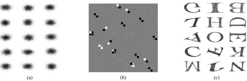
Figure 4: Illustration of the JFD method on the uBSSD task for the 3D-geom database. Sample number T =100,000, convolution length L=1, Amari-index: 0.25%. (a): observed convolved signals x(t). (b) Hinton-diagram: the product of the mixing matrix of the derived ISA task and the estimated demixing matrix (= approximately block-permutation matrix with 3×3 blocks). (c): estimated components. Note: hidden components are recovered L+L0=2 times, up to permutation and orthogonal transformation.

(a) (b) (c)

Figure 5: Illustration of the JFD method on the uBSSD task for the celebrities database. Sample number T =100,000, convolution length L=1, Amari-index: 0.37%. (a): observed convolved signals x(t). (b) Hinton-diagram: the product of the mixing matrix of the derived ISA task and the estimated demixing matrix (= approximately block-permutation matrix with 2×2 blocks). (c): estimated components. Note: hidden components are recovered L+L0=2 times, up to permutation and orthogonal transformation.

SZABO´, P ´OCZOS ANDL ˝ORINCZ

1 2 5 10 30 50 75

10−2 10−1 100

Number of samples (T)

Amari−index

uBSSD: ABC (JFD)

L=1, D ISA=8 L=2, D_ISA=16 L=5, D_ISA=40 L=10, D_ISA=80 L=20, D_ISA=160 L=30, D_ISA=240

x103

(a)

1 2 5 10 20 30

0 2 4 6 8

L

Number of sweeps

uBSSD: ABC (JFD)

min mean max

(b)

Figure 6: (a): Amari-index of the JFD method on the ABC database as a function of sample number and for different convolution lengths on log-log scale. (b): Number of sweeps of permutation optimization on the derived ISA task as a function of convolution length. Dimension of the ISA task: DISA. Black: minimum, gray: average, light gray: maximum. For further information, see Table 4.

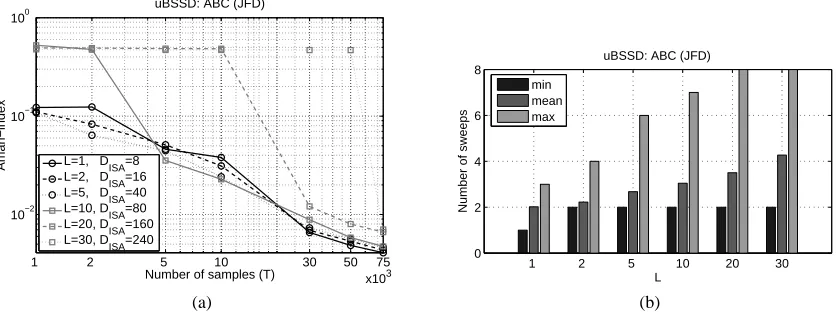
In another test the ABC database was used. The number and the dimensions of the components were minimal (d=2, M=2) and the dependence on the convolution length was tested. Parameter L took values on 1,2,5,10,20,30. The number of observations varied between 1,000≤T ≤75,000. The Amari-index and the sweep number of the optimization are illustrated in Figure 6. Precise values of the Amari-index are provided in Table 4.

L=1 L=2 L=5 L=10 L=20 L=30

0.41%(±0.06)0.44%(±0.05)0.46%(±0.05)0.47%(±0.03)0.66%(±0.13)0.70%(±0.11)

Table 4: Amari-index of the JFD method for ABC database for different convolution lengths: average ± deviation. Number of samples: T =75,000. For other sample numbers between 1,000≤T <75,000 see Figure 6(a).

According to Figure 6, the JFD method found the hidden components. The ‘power law’ decline of the Amari-index, which was apparent in the 3D-geom and the celebrities databases, appears for the ABC test, too. The figure indicates that for 75,000 samples and for L=30 (convolution length is 31) the problem is still amenable to the JFD technique. The number of sweeps required for the optimization of the permutations was between 1 and 8 for all sample numbers 1,000≤T ≤75,000, parameters 1≤L≤30 and for all 50 random initializations. According to Table 4, for sample number T =75,000 the Amari-index stays below 1% on average (0.41−0.7%) and has a small (0.03−0.11) standard deviation.

1 2 5 10 30 50 75 10−2

10−1 100

Number of samples (T)

Amari−index

uBSSD: Beatles (JFD)

L=1, D_ISA=8

L=2, D_ISA=16

L=5, D_ISA=40

L=10, D_ISA=80

L=20, D_ISA=160

L=30, D_ISA=240

x103

(a)

1 2 5 10 20 30

0 1 2 3 4 5 6

L

Number of sweeps

uBSSD: Beatles (JFD)

min mean max

(b)

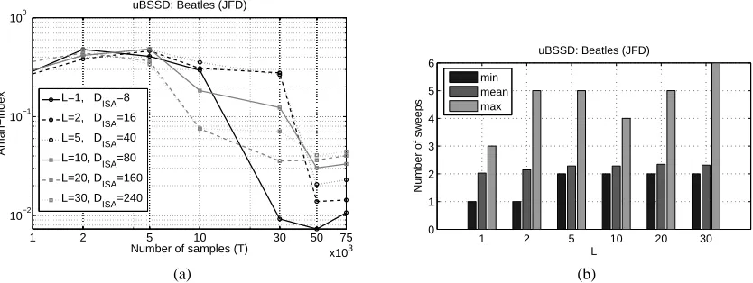
Figure 7: (a): Amari-index of the JFD method on the Beatles database as a function of sample num-ber and for different convolution lengths on log-log scale. (b): Numnum-ber of sweeps of permutation optimization on the derived ISA task as a function of convolution length. Dimension of the ISA task: DISA. Black: minimum, gray: average, light gray: maximum. For further information, see Table 5.

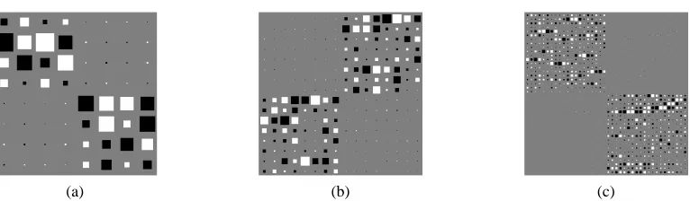
optimization are illustrated in Figure 7. Precise values of the Amari-index are provided in Table 5. The Hinton-diagrams are in Figure 8.

The Beatles songs are non-i.i.d sources and subsequent samples sm(t) and sm(t−1)have depen-dencies. Thus, in S(t) the components of the (6) model that belong to the same song can not be distinguished. In the ideal case, however, the songs can be separated, that is, the separation of the 2 pieces of(DISA/2)-dimensional song-subspaces is possible. We measure the appearance of the 2 of(DISA/2)-dimensional blocks for the Beatles songs by means of the Amari-index. The results, which demonstrate the success of our method, are shown in Figure 7. It can be seen that the JFD method found the hidden components, for 50 and 75 thousand samples for L=30 (convolution length is 31) too. The number of sweeps required for the optimization of the permutations was between 1 and 6 for all sample numbers 1,000≤T ≤75,000, parameters 1≤L≤30 and for all 50 random initializations. According to Table 5, for sample number T=75,000 the Amari-index is between 1.07%(L=1)and 4.43%(L=30)on the average and has a small (0.04−0.09) standard deviation. Separation of the 2 of DISA/2 dimensional subspaces are illustrated in Figure 8 through the Hinton-diagrams.

L=1 L=2 L=5 L=10 L=20 L=30

1.07%(±0.04)1.43%(±0.09)2.29%(±0.07)3.31%(±0.06)4.03%(±0.06)4.43%(±0.04)

(a) (b) (c)

Figure 8: Hinton-diagrams of the JFD methods on the Beatles database for different convolution parameters. (a): L=1(DISA=8), (b): L=2(DISA=16), (c): L=5(DISA=40). In the ideal case, 2 pieces of DISA/2-dimensional blocks are formed by multiplying the mixing matrix of the derived ISA task and the estimated demixing matrix.

5.3.2 KERNEL-ISA TECHNIQUES

We study the efficiency of the KCCA and KGV ISA methods of Section 4.1.2. The kernel-ISA techniques was found to have a higher computational burden, but they also have advantages compared with the JFD technique for ISA tasks.

For the KCCA and KGV methods we also applied the pseudocode of Table 2. ICA was executed by the fastICA algorithm (Hyv¨arinen and Oja, 1997). The Gaussian kernel k(u,v)∝exp−ku_2σ−2vk2

was chosen for both the KCCA and KGV methods and parameter σwas set to 5. In the KCCA method, regularization parameterκ=10−4was applied. In the experiments, parameters(σ,κ)were proved to be reasonably robust. Mixing matrix A was generated randomly from the orthogonal group and the sample number was chosen from the interval 100≤T ≤5,000.

Our first ISA example concerns the ABC database. The dimension of a component was d=2 and the number of the components M took different values (M =2,5,10,15). Precision of the estimations is shown in Figure 9, where the precision of the JFD method on the same database is also depicted. The number of sweeps required for the optimization of the permutations is shown in Figure 10 for different sample numbers and for different component numbers. The data are averaged over 50 random estimations. Figure 11 depicts the KCCA estimation for the ABC database.

Figure 9 shows that the KCCA and KGV kernel-ISA methods give rise to high precision esti-mations on the ABC database even for small sample numbers. The KGV method was more precise for all M values studied than the JFD method. The ratio of precisions could be as high as 4 (see sample number 500). The KCCA method is somewhat weaker. For smaller tasks (M=2 and 5) and for small sample numbers it also exceeds the precision of the JFD method. Precision of the method become about the same for higher sample numbers and larger tasks. Sweep numbers of the KCCA (KGV) method were between 2 and 8 (2 and 6) (Figure 10). Note that one sweep is always necessary for our procedure (Table 2). A single sweep may be satisfactory if—by chance—the ICA provides the correct permutation.

100 200 500 1000 2000 5000 10−1

100

Number of samples (T)

Amari−index

ISA: ABC (KCCA)

M=2 M=5 M=10 M=15

(a)

100 200 500 1000 2000 5000

10−1 100

Number of samples (T)

Amari−index

ISA: ABC (KGV)

M=2 M=5 M=10 M=15

(b)

100 0 200 500 1000 2000 5000

1 2 3 4 5

Number of samples (T)

Quotient of Amari−indices

ISA: ABC (JFD/KCCA)

M=2 M=5 M=10 M=15

(c)

100 0 200 500 1000 2000 5000

1 2 3 4 5

Number of samples (T)

Quotient of Amari−indices

ISA: ABC (JFD/KGV)

M=2 M=5 M=10 M=15

(d)

Figure 9: (a) and (b): Amari-index of the KCCA and KGV methods, respectively, for the ABC database as a function of sample number and for different numbers of components M. (c) and (d): Amari-index of the JFD method is divided by the Amari-index of the KCCA method and the KGV technique, respectively. For values larger (smaller) than 1 the kernel-ISA method is better (worse) than the JFD method.

M=2 M=5 M=10 M=15

KCCA 1.33%(±0.48) 1.20%(±0.17) 2.76%(±2.86) 3.00%(±2.21)

KGV 1.26%(±0.54) 1.18%(±0.17) 1.51%(±0.31) 1.54%(±0.34)

Table 6: Amari-index for the KCCA and the KGV methods for database ABC, for different compo-nent number M: average±deviation. Number of samples: T =5,000. For other sample numbers between 100≤T <5,000, see Figure 9.

2 5 10 15 0

2 4 6 8

M

Number of sweeps

ISA: ABC (KCCA)

min mean max

(a)

2 5 10 15

0 1 2 3 4 5 6

M

Number of sweeps

ISA: ABC (KGV)

min mean max

(b)

Figure 10: Number of sweeps for the KCCA and the KGV methods needed for the optimization of permutations as a function of component number M on the ABC database. (a): KCCA method, (b): KGV method. Black: minimum, gray: mean, light gray: maximum.

(a) (b) (c)

Figure 11: Illustration of the KCCA method for the ABC database. Sample number: T =5,000. (a): observed mixed signals x(t). (b) Hinton-diagram: the product of the mixing matrix of the derived ISA task and the estimated demixing matrix (= approximately block-permutation matrix). (c): estimated components. Hidden components are recovered up to permutation and orthogonal transformation.

According to Figure 12 the two kernel-based methods exhibit similar precision. Both were superior to the JFD technique. The ratio of the Amari-indices for sample number 5,000 and for

k=2 is more than 15,000, for k=3 it is more than 500. For details concerning the Amari-indices, see Table 7. These indices are close to each other for the KCCA and the KGV methods: 0.0017% for

k=2, 0.16% for k=3 on average. Both kernel-ISA methods used 2−3 sweeps for the optimization of the permutations (Figure 13).

6. Conclusions

100 200 500 1000 2000 5000 10−4

10−3 10−2 10−1 100

Number of samples (T)

Amari−index

ISA: all−k−independent (KCCA)

k=2 k=3

(a)

100 200 500 1000 2000 5000

10−4 10−3 10−2 10−1 100

Number of samples (T)

Amari−index

ISA: all−k−independent (KGV)

k=2 k=3

(b)

100 200 500 1000 2000 5000

101 102 103 104

Number of samples (T)

Quotient of Amari−indices

ISA: all−k−independent (JFD/KCCA)

k=2 k=3

(c)

100 200 500 1000 2000 5000

101 102 103 104

Number of samples (T)

Quotient of Amari−indices

ISA: all−k−independent (JFD/KGV)

k=2 k=3

(d)

Figure 12: (a) and (b): Amari-indices of the KCCA and KGV methods, respectively, as a function of the sample number and for k=2 and 3 on the all-k-independent database. For more details, see Table 7. (c): ratio of Amari-indices of JFD and KCCA methods, (d): ratio of Amari-indices of JFD and KGV methods.

2 3

0 1 2 3

k

Number of sweeps

ISA: all−k−independent (KCCA)

min mean max

(a)

2 3

0 1 2 3

k

Number of sweeps

ISA: all−k−independent (KGV)

min mean max

(b)

k=2 k=3 KCCA/KGV 0.0017%(±0.0014) 0.16%(±0.04)

Table 7: The Amari-index of the KCCA and KGV methods for database all-k-independent for different k values: average±deviation. Number of samples: T =5,000. For other sample numbers between 100≤T <5,000, see Figure 12.

undercomplete version (uBSSD) of the task has been presented, and it has been shown how to derive an independent subspace analysis (ISA) task from the uBSSD problem. Recent developments of the ISA techniques enabled us to handle the emerging high dimensional problems. Our earlier results, namely the ISA Separation Theorem (Szab ´o et al., 2006b) motivated us to reduce the ISA task to the search for the optimal permutation of the ICA components. The components were grouped with a novel joint decorrelation technique, the joint f-decorrelation (JFD) method (Szab ´o and L˝orincz, 2006).

Also, we adapted other ICA techniques, such as the KCCA and KGV methods to the ISA task and studied their efficiency. Simulations indicated that although the KCCA and KGV methods give rise to serious computational burden relative to the JFD method, they can be advantageous for smaller ISA tasks and for ISA tasks when the number of samples is small.

Finally, we note that we achieved small errors in these high dimensional computations. These small errors indicate that the Separation Theorem is robust and might be extended to a larger class of noise sources.

Acknowledgments

The authors would like to thank Katalin L´az´ar and G´abor Szirtes for reading the manuscript, and for their valuable suggestions. We furthermore thank the anonymous reviewers for their helpful comments.

Appendix A. Proof of the ISA Separation Theorem

We shall rely on entropy inequalities (Section A.1). In Section A.2 connection to the ICA cost function is derived (Lemma 2). The ISA Separation Theorem then follows.

A.1 EPI-type Relations

First, consider the so-called entropy power inequality (EPI)

e2H(∑Li=1ui)_≥

L

∑

e2H(ui),

where u1, . . . ,uL ∈Rdenote continuous random variables. This inequality holds, for example, for independent continuous variables (Cover and Thomas, 1991).