Segmental Hidden Markov Models with Random Effects for Waveform Modeling

Segmental Hidden Markov Models with Random Effects for

Waveform Modeling

Seyoung Kim [email protected]

Department of Computer Science University of California, Irvine Irvine, CA 92697-3425, USA

Padhraic Smyth [email protected]

Department of Computer Science University of California, Irvine Irvine, CA 92697-3425, USA

Editor: Sam Roweis

Abstract

This paper proposes a general probabilistic framework for shape-based modeling and classification of waveform data. A segmental hidden Markov model (HMM) is used to characterize waveform shape and shape variation is captured by adding random effects to the segmental model. The resulting probabilistic framework provides a basis for learning of waveform models from data as well as parsing and recognition of new waveforms. Expectation-maximization (EM) algorithms are derived and investigated for fitting such models to data. In particular, the “expectation conditional maximization either” (ECME) algorithm is shown to provide significantly faster convergence than a standard EM procedure. Experimental results on two real-world data sets demonstrate that the proposed approach leads to improved accuracy in classification and segmentation when compared to alternatives such as Euclidean distance matching, dynamic time warping, and segmental HMMs without random effects.

Keywords: waveform recognition, random effects, segmental hidden Markov models, EM

algo-rithm, ECME

1. Introduction

Automatically parsing and recognizing waveforms based on their shape has broad applications, including interpretation and classification of heartbeats in ECG data analysis (Koski, 1996), analysis of waveforms from turbulent flow experiments (Bruun, 1995), and discrimination of nuclear events and earthquakes in seismograph data (Bennett and Murphy, 1986). Waveform analysis has also attracted attention in information retrieval and data mining, with a focus on algorithms that can take a waveform as an input query and search a large database to find similar waveforms that match the query waveform (e.g., Yi and Faloutsos, 2000). Applications include finding temporal patterns in retail time-series data (Agrawal et al., 1993) and fault diagnosis in complex systems (Keogh and Smyth, 1997).

0 50 100 150 200 250 −3

−2 −1 0 1 2 3

time

y (measurements)

0 50 100 150 200 250 −3

−2 −1 0 1 2 3

time

y (measurements)

(a) (b)

0 50 100 150 200 250 −3

−2 −1 0 1 2 3

time

y (measurements)

0 50 100 150 200 250 −3

−2 −1 0 1 2 3

time

y (measurements)

(c) (d)

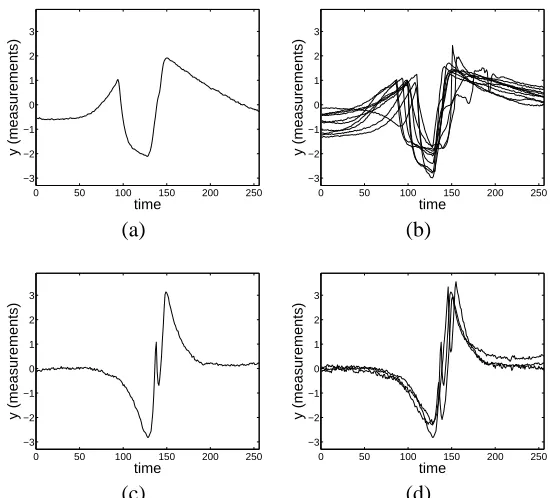
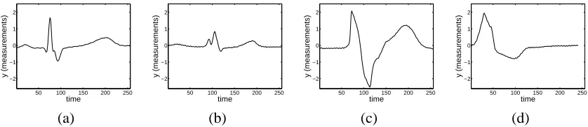
Figure 1: Fluid-flow waveform data: (a) a waveform from the class splitting (where the probe splits a bubble), (b) a set of such waveforms, (c) a waveform from the class glance, and (d) a set of such waveforms.

interactions between a probe and bubbles in the fluid. Figure 1(a) shows an example waveform from a particular type of interaction. Figure 1(b) shows a whole set of such waveforms that have all been classified (by human experts) as being of the same interaction type. Although all of these waveforms belong to the same interaction class, there is significant variability in shape among those waveforms. The sources of variability include shifts of the locations of prominent features such as peaks, valleys, and plateaus, scaling along the time and amplitude axes, and measurement noise. An example waveform from a different class is shown in Figure 1(c), and a set of such waveforms are shown in Figure 1(d). Again there is significant within-class variability.

In this paper we address the problem of detecting and classifying general classes of waveforms based on their shape and propose a new statistical model that directly addresses within-class shape variability. We will assume in the paper that the waveforms to be analyzed are in the form of “snippets” that have already been extracted from the “background” time-series, e.g., in the form of Figures 1(b) and (d). This assumption can be relaxed—we outline a method for detection of waveforms that are embedded in a time-series in Section 6. We will also assume that the waveforms are being analyzed offline, i.e., that all of the waveform measurements are available at the time of analysis rather than arriving sequentially in an online fashion. The online sequential detection problem can be addressed by generalizing the methods we propose, but we do not pursue online algorithms in this paper.

0 50 100 150 200 250 −3

−2 −1 0 1 2 3

time

y (measurements)

0 50 100 150 200 250 −3

−2 −1 0 1 2 3

time

y (measurements)

segmental HMMs waveform data

0 50 100 150 200 250 −3

−2 −1 0 1 2 3

time

y (measurements)

random effects segmental HMMs waveform data

(a) (b) (c)

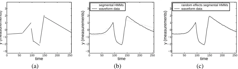
Figure 2: Waveform models: (a) a piecewise linear approximation of the waveform in Figure 1(a), (b) a segmental HMM best fit, and (c) a random effects segmental HMM best fit as de-scribed in this paper.

modeling, finding application (for example) in heartbeat monitoring of ECG data (Koski, 1996; Hughes et al., 2003). These models are characterized by (a) a discrete-time finite-state Markov process which is unobserved, and (b) a set of observed measurements at each time t which only depend (stochastically) on the state value at time t. From a shape-modeling viewpoint the standard version of the model generates noisy versions of piecewise constant shapes over time, since the observations within a sequence of states of the same value have constant mean. For waveform modeling, a useful extension is the so-called segmental HMM, originally introduced in the speech recognition (Russell, 1993) and more recently used for more general waveform modeling (Ge and Smyth, 2000). The segmental model allows for the observed data within each segment (a sequence of states with the same value) to follow a general parametric regression form, such as a linear function of time with additive noise. This allows us to model the shape of the waveform directly, in this case as a sequence of piecewise linear components—Figure 2(a) shows a piecewise linear representation of the waveform in Figure 1(a).

A limitation of this particular model is that it assumes that the parameters of the model are fixed. Thus, the only source of variability in an observed waveform arises from variation in the lengths of the segments and observation noise added to the functional form in each segment. The limitation of this can clearly be seen in Figure 2(b), where a segmental HMM has been trained on the data in Figure 1(b) and then used to generate maximum-likelihood estimates of segment boundaries, slopes, and intercepts for the new waveform in Figure 2(b). We can see that the best-fit slopes and intercepts provided by the model do not match the observed data particularly well in each segment, e.g., in the first segment the intercept is clearly too low on the y-axis, in the second segment the slope is too small, and so forth. By using the same fixed parameters for all waveforms, the model cannot fully account for variability in waveform shapes (e.g., as seen in Figure 1(b)).

template (at the top level) modeled as a population prior. The parameters of this prior can be learned in an unsupervised manner from data in the form of sets of waveforms. The resulting model can be viewed as a directed graphical model, allowing for application of standard methods for inference and learning (Jordan, 1999; Murphy, 2002). For example, we can in principle learn that the slopes across multiple waveforms for the first segment in Figure 1(b) tend to have a characteristic mean slope and standard deviation. The random effects approach provides a systematic mechanism for allowing variation in “shape space” in a manner that can be parametrized. Figure 2(c) shows a visual example of how a random effects model (constructed from the training data in Figure 1(b)) is used to generate maximum-likelihood estimates of segment boundaries and segment slopes and intercepts for the waveform in Figure 1(a).

Kim et al. (2004) described preliminary results using random effects segmental HMMs for waveform parsing and recognition. A drawback of this earlier approach is the relatively slow con-vergence of the expectation-maximization (EM) algorithm in learning. This is a result of the large amount of missing information present (due to the random effects component of the model), com-pared to a standard segmental HMM. In this paper we use the “expectation conditional maximization either” (ECME) algorithm (Liu and Rubin, 1994) for parameter estimation of random effects seg-mental HMMs. This dramatically speeds up convergence relative to the EM algorithm, making the model much more practical to use for real-world waveform recognition problems.

We begin our discussion by reviewing related work on segmental HMMs and random effects models in Section 2. We introduce segmental HMMs in Section 3. In Section 4, we extend this model to incorporate random effects models, and describe the inference procedure and the EM algorithm for parameter estimation. We also show that the ECME algorithm can be used to signifi-cantly speed up the convergence of the EM algorithm. In Section 5, we evaluate our model on two applications involving bubble-probe interaction data and ECG data, and compare random effects segmental HMMs to other waveform-matching algorithms such as Euclidean distance matching, dynamic time warping, and segmental HMMs without random effects. Section 6 contains a brief discussion of possible extensions of the model and final conclusions.

2. Related Work and Contributions

to learn models from data, to handle within-class waveform variability, and to generate maximum-likelihood segmentations of waveforms.

As mentioned in Section 1, standard discrete-time finite-state HMMs are not ideal for modeling waveform shapes since the generative model implicitly assumes a geometric distribution on segment lengths and a piecewise constant shape model. Segmental HMMs relax these modeling constraints by allowing (a) arbitrary distributions on run lengths, and (b) “segment models” (regression mod-els) that allow the mean to be a function of time within each segment. HMMs that allow arbitrary distributions on run lengths (the semi-Markov property in a HMM context) were introduced in the work of Ferguson (1980), Russell and Moore (1985), and Levinson (1986). Deng et al. (1994) and Russell (1993) extended these models to segmental HMMs by modeling dependencies between ob-servations from the same state with a parametric trajectory model that changes over time. Ostendorf et al. (1996) reviewed variations of segmental HMMs from a speech recognition perspective. More recent work includes Achan et al. (2005) and Yun and Oh (2000). Ge and Smyth (2000) introduced the idea of using segmental HMMs for general waveform recognition problems.

The idea of using random effects with segmental HMMs to model parameter variability across waveforms is implicit in the speech recognition work of both Gales and Young (1993) and, later, Holmes and Russell (1999). This work can be viewed as precursors to the more general random effects segmental HMM framework we present in this paper. Gales and Young (1993) used a model with a constant mean per segment, but where the mean values themselves come from a distribution, allowing modeling of variability across different individual speakers. Holmes and Russell (1999) extended this idea to use a linear regression function instead of a constant mean for each segment with a Gaussian prior on the regression parameters (slope and intercept) for each segment. In earlier work (Kim et al., 2004), we noted that Holmes and Russell’s model could be formalized within a random effects framework, and derived a more general EM framework for such models, taking advantage of ideas developed separately in speech recognition and in statistics.

In the statistical literature there is a significant body of work on modeling a hierarchical data-generating process with a random effects model and estimating the parameters of this model (Searle et al., 1992). Dempster et al. (1977) sketched the EM algorithm for finding maximum-likelihood estimates for parameters of random effects models. This algorithm was further developed by Demp-ster et al. (1981), Laird and Ware (1982), and Laird et al. (1987). There appears to be no work in the statistical literature on applying random effects to segmental HMMs.

In this context, the primary contribution of this paper is a general framework for random-effects segmental hidden Markov models. We demonstrate how such models can be used for waveform modeling, recognition, and segmentation, with experimental comparisons of the random effects approach with alternative methods such as dynamic time warping, using two real-world data sets. We extend earlier approaches for learning the parameters of random effects segmental HMMs by deriving a provably correct EM algorithm with monotonic convergence. Both Gales and Young (1993) and Holmes and Russell (1999) derived EM-like optimization algorithms, but their M steps are not in a closed form and use approximate solutions—thus, the monotonic convergence property of EM is not guaranteed in general using their approaches.

inference algorithm (applicable to both EM and ECME) that reduces the time complexity of the

forward-backward algorithm by a factor of T2, where T is the length of a waveform. We also show

that this inference algorithm can be applied to full covariance models rather than assuming (as in Holmes and Russell, 1999) that the intercept and slope in the segment distribution are conditionally independent. Since the inference algorithm is used in each iteration of the E step in the EM and ECME iterations, this significantly reduces the overall time complexity of each iteration of EM and ECME.

3. Segmental HMMs

A segmental HMM with M states is described by an M×M transition matrix, a probability

distri-bution over duration for each state, and a segment model for each state. The transition matrix A (assumed here to be stationary in time) has entries akl, namely, the probability of being in state l at

time t+1 given state k at time t. The initial state distribution can be included in A as transitions from a special state 0 to each state k=1, . . . ,M. In waveform modeling, we typically constrain the transition matrix to allow only left-to-right transitions and do not allow self-transitions. Thus, there is an ordering on states, each state can be visited at most once, and states can be skipped.

In this paper, we model the duration distribution of state k using a Poisson distribution,

P(d−1|λk) =

e−λkλ kd−1

(d−1)! d=1,2, . . .

(shifted to start at d=1 to prevent a silent state). Other choices for the duration distribution could also be used (e.g., Ferguson, 1980; Levinson, 1986). Once the process enters state k, a duration d is drawn, and state k produces a segment of observations of length d from the segment distribution model. In this paper we focus on models with linear functional forms within each segment. We model the rth segment of observations of length d, yr, generated by state k, as a linear function of

time,

yr=Xrβk+er er∼Nd(0,σ2Id), (1)

whereβ_kis a 2×1 vector of regression coefficients for the intercept and slope, eris a d×1 vector of

Gaussian noise with varianceσ2_{for each component, and X}

ris a d×2 design matrix consisting of

a column of 1’s (for the intercept term) and a column of x values representing discrete time values. In speech recognition using the mid-point of a segment as a parameter in the model instead of intercept has been shown to lead to better speech recognition performance (Holmes and Russell, 1999). Nonetheless, parametrization of the model via the intercept worked well in our experiments, and for this reason we use the intercept in the models discussed in this paper. For simplicity,σ2is assumed to be common across all states; again this can be relaxed. We do not enforce continuity of the mean functions (Equation (1)) across segments in the probabilistic model. However, as re-ported in Section 5, the model without continuity constraints worked well on real-world data in our recognition experiments.

Treating the unobserved state sequences as missing, we can estimate the parameters,θ={A,Λ=

{λk|k=1, . . . ,M},θf={βk,(σ2)|k=1, . . . ,M}}, using the EM algorithm, with the forward-backward

dis-tribution, recursively computes

αt(k) =P(y1:t,state k ends at t|θ)

α∗

t(k) =P(y1:t,state k starts at t+1|θ) (2)

in the forward pass, and

βt(k) =P(yt+1:T|state k ends at t,θ)

β∗

t(k) =P(yt+1:T|state k starts at t+1,θ) (3)

in the backward pass, and returns the results to the M step as a set of sufficient statistics (Rabiner and Juang, 1993).

Inference algorithms for segmental HMMs provide a natural way to evaluate the performance of the model on test data. The F-B algorithm scores a previously unseen waveform y by calculating the likelihood

p(y|θ) =

∑

s

p(y,s|θ) =

∑

k

αT(k), (4)

where s represents a sequence of unknown state labels for observations y. The Viterbi algorithm can provide a segmentation of a waveform by computing the most likely state sequence (e.g., Figure 2(b)). The addition of duration distributions in segmental HMMs increases the time complexity of both the F-B and Viterbi algorithms from O(M2T)for standard HMMs to O(M2T2), where T is the length of the waveform (i.e., the number of observations).

4. Segmental HMMs with Random Effects

A random effects model is a general statistical framework when the data generation process has a hierarchical structure, coupling a population-level model with individual-level variation. At each level of the generative process, the model defines a prior distribution over the individual group pa-rameters, called random effects, of one level below. The observed data are generated at the bottom of the hierarchy, given parameters drawn from the prior distribution one level above. Typically, the random effects are not observable, so the EM algorithm is a popular approach to learning model parameters from the observed data (Dempster et al., 1981; Laird and Ware, 1982). By combin-ing segmental HMMs and random effects models we can take advantage of the strength of each in waveform modeling. Random effects models add one level of hierarchy to the probabilistic struc-ture of segmental HMMs, defining a population distribution over the possible shapes of waveform segments. Instead of requiring all waveforms to be modeled with a single set of parameters, indi-vidual waveforms are allowed to have their own parameters but coupled by a common population prior across all waveforms.

4.1 The Model

Beginning with the segmental HMMs described in Section 3, we add random effects via a new variable ui_rto the segment distribution part of the model as follows. Consider the rth segment yi_rof

Templateβ_k’s

+ _{? @@R} QQs

(β_k + ˆui_r)’s for

ith waveform i=1, . . . ,5

? ? ? ? ?

Observed data

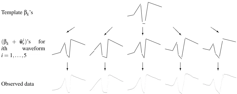
Figure 3: A visual illustration of the random effects segmental HMM, using fluid-flow waveform data as an example (as described in Section 5.1). The top level shows the population level parametersβ_k’s for the waveform shape. The plots at the bottom level consist of observed data. The plots in the middle level show the posterior estimates (combining both the data and the prior) of ˆuiand ˆsi, using Equation (8) and the Viterbi algorithm respectively.

and Ware (1982), we describe the generative model as a two-level process. At the bottom level, we model the observed data yi_ras

yi_r=Xi_rβ_k+Xi_rui_r+ei_r ei_r∼Nd(0,σ2Id), (5)

where ei_r is the measurement noise, Xi_r is a d×2 design matrix for the time measurements

cor-responding to yi_r, (β_k+ui_r) are the regression coefficients, and 1≤i≤N (for N waveforms). β_k represents the mean regression parameters for segment k, and ui_rrepresents the variation in regres-sion (or shape) parameters for the ith individual waveform. At this level, the individual random effects ui_ras well asβ_kandσ2are viewed as parameters. At the top level, ui_ris viewed as a random variable with distribution

ui_r∼N2(0,Ψk), (6)

whereΨkis a 2×2 covariance matrix, and uiris independent of eir. Notice that this model described

by Equations (5) and (6) is equivalent to having yi_r=Xi_rβi_r+ei_r with βi_r∼N2(βk,Ψk). It can be

shown that yi_rand ui_rhave the following joint distribution:

yi_r ui_r

∼Nd+2

Xi_rβ_k 0

,

Xi_rΨkXir ′

+σ2_I

d XirΨk

ΨkXir

′ _Ψ

k

. (7)

Also, from Equation (7), the posterior distribution of ui

rcan be written as

ui_r|yi_r,β_k,Ψk,σ2∼N2 ˆuir,Ψˆui r

, (8)

where

ˆui_r= (Xi_r′Xi_r+σ2(Ψk)−1)−1Xir ′

yi_t

X_ti

β_k σ2

t=1 : D i=1 : N

?

ui_r

Ψk

-?

i=1 : N

yi_t

Xi_t

β_k σ2

t=1 : D

?

Ψk

i=1 : N

y_ti

Xi_t

β_k σ2

t=1 : D

? @

@ @_@R

(a) (b) (c)

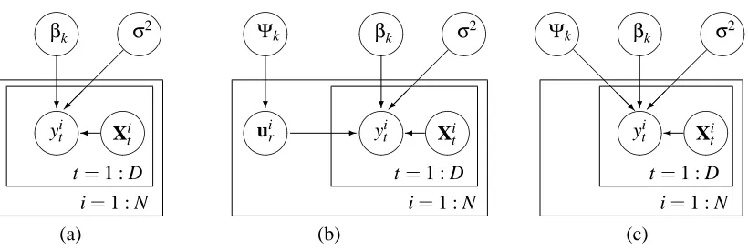
Figure 4: Plate diagrams for the segment distribution part of segmental HMMs and random effects segmental HMMs. (a) segment model in segmental HMMs, (b) a two-stage model with random effects parameters in random effects segmental HMMs, and (c) the model after integrating out random effects parameters from (b).

and

Ψˆui r =σ

2_(Xi r ′

Xi_r+σ2(Ψk)−1) −1

. (10)

In the discussion that follows we use ui to denote{ui_r|r=1, . . . ,R}given the segmentation si of waveform yi into R segments. Similarly, ˆui represents{ˆu_ri|r=1, . . . ,R}, given the segmentation ˆsi

of waveform yifound by the Viterbi algorithm.

Figure 3 conceptually illustrates the hierarchical setup of the model. The shape template

de-scribed by the population parametersβ_k’s is shown at the top of the hierarchy. The plots at the

bottom level consist of observed data. The plots at the middle level show the posterior estimates (combining both the data and the prior) of ˆuiand ˆsi, using Equation (8) and the Viterbi algorithm re-spectively. From a generative model perspective, the shape templates in the middle row,(β_k+ui_r)’s,

i=1, . . . ,5, are generated from the mean shape at the top level by Equation (6). The observed data

at the bottom of the hierarchy are modeled as noisy realizations of these individual shape templates. This final data generation process is modeled in Equation (5).

Figure 4 shows plate diagrams for the segment distribution part of segmental HMMs and random effects segmental HMMs, illustrating the generative process for N waveforms, y1, . . . ,yN, under the simplifying assumption that each waveform comes from a single segment of length D corresponding to state k.

4.2 Inference

To handle the random effects component in the F-B and Viterbi algorithms for segmental HMMs,

we notice from Equation (7) that the marginal distribution of a segment yi_r generated by state k

is Nd(Xirβk,XirΨkXir ′

+σ2_I

d), and that this corresponds to Equation (1) with the covariance matrix

σ2_I

dreplaced by(XirΨkXir ′

+σ2_I

d). Replacing the two-level segment distribution with this marginal

distribution, and collapsing the hierarchy into a single level, we can use the same F-B and Viterbi

The F-B algorithm recursively computes the quantities in Equations (2) and (3). These are then used in the M step of the EM algorithm. The likelihood of a waveform y, given fixed parameters

θ={A,Λ,θf ={βk,Ψk,(σ2)|k=1, . . . ,M}}, but with states s and random effects u unknown, is

evaluated as

p(y|θ) =

∑

s Z

p(y,s,u|θ)du (11)

=

∑

s

p(y,s|θ) =

∑

k

αT(k).

As in segmental HMMs, the Viterbi algorithm can be used as a method to segment a waveform by computing the most likely state sequence.

What appears to make the inference in random effects segmental HMMs computationally much

more expensive than in segmental HMMs is the inversion of the d×d covariance matrix of the

marginal segment distribution, Xi_rΨkXir ′

+σ2_I

d, during the evaluation of the likelihood of a

seg-ment. For example, in the F-B algorithm, the likelihood of a segment yi_r of length d given state k,

p(yi_r|β_k,Ψk,σ2), needs to be calculated for all possible durations d in each of theαt(k) andβt(k)

expressions at each recursion. Naive computation of a segment likelihood, using direct inversion of

the d×d covariance matrix, requires O(T3)computations, where T is the upper bound for d,

lead-ing to an overall time complexity of O(M2T5). This can be computationally impractical for long

waveforms with a large value of T (for example, T =256 for the fluid-flow data shown in Figure

1(a)).

In the case of a simpler model with a diagonal covariance matrix forΨk, Holmes and Russell

(1999) derived a method for computing the segment likelihood with time complexity O(M2T3). We

obtain the same complexity for a more general case with an arbitrary covariance matrix as follows. In discussing computational issues for random effects models, Dempster et al. (1981) suggested an expression for the likelihood that is simple to evaluate. Applying their method to the segment

distribution of our model, we rewrite, using Bayes’ rule, the likelihood of a segment yi_rgenerated

by state k as

p(yi_r|β_k,Ψk) =

p(yi_r,ui_r|β_k,Ψk,σ2)

p(ui

r|yir,βk,Ψk,σ2)

,

where the numerator and the denominator of the right-hand side are given as Equations (7) and (8), respectively. The right-hand side of the above equation holds for all values of ui_r. By setting ui_rto

ˆui

ras in Equation (9), we can simplify the expression for the segment likelihood to

p(yi_r|β_k,Ψk) = (2π)−d/2σ−d|Ψˆui r|

1/2_/|Ψ

k|1/2exp(−Sir/(2σ2)), (12)

where

Si_r= (yi_r−Xi_rβ_k−Xi_rˆui_r)′(yi_r−Xi_rβ_k−Xi_rˆui_r) +σ2ˆui_r′Ψ(_k−1)ˆui_r. This can be further simplified using Equation (9):

Si_r= (yi_r−Xi_rβ_k)′(yi_r−Xi_rβ_k−Xi_rˆui_r).

Equation (12) has a form that involves only O(d)computations for each step, where previously this

time complexities of the F-B and Viterbi algorithms are reduced to O(M2T3). For segmental HMMs

this computational complexity can be further reduced to O(M2T2) by precomputing the segment

likelihood and storing the values in a table (Mitchell et al., 1995). However, this precomputation is not possible with random effects models, leading to the additional factor of T in the complexity term.

4.3 Parameter Estimation

In this section, we describe how to obtain maximum-likelihood estimates of the parameters from a training set of multiple waveforms for a random effects segmental HMM using the EM algorithm. We augment the observed waveform data with both (a) state sequences and (b) random effects parameters (both are considered to be hidden). The log likelihood of the complete data of N wave-forms, D_complete= (Y,S,U) ={(y1,s1,u1), . . . ,(yN,sN,uN)}, where the state sequence si implies Risegments in waveform yi, is defined as:

log L(θ|D_complete) =

N

∑

log p(yi,si,ui|A,Λ,θf)

=

N

∑

Ri

∑

log P(si_r|si_r−1,A) (13a)

+

N

∑

Ri

∑

log P(d_ri|λk,k=sir) (13b)

+

N

∑

Ri

∑

log p(yi_r|ui_r,β_k,σ2_,k=si

r,dri) (13c)

+

N

∑

Ri

∑

log p(ui_r|Ψk,k=sir). (13d)

As we can see from the above equation, given the complete data, the log-likelihood decouples into four parts Equations (13a)-(13d), where the transition matrix, the duration distribution parameters, the bottom level parametersβ_k,σ2_{, and the top level random effect parameters u}i

rappear in each of

the four terms. If we had complete data, we could optimize the four sets of parameters indepen-dently. When only parts of the data are observed, by iterating between the E step and the M step in the EM algorithm as described below, we can find a solution that locally maximizes the likelihood of the observed data.

4.3.1 E STEP

In the E step, we find the expected log likelihood of the complete data,

Q(θ(t),θ) =E[log L(θ|D_complete)], (14)

with respect to

p(S,U|Y,θ(t)) = p(U|S,Y,θ(t))P(S|Y,θ(t))

=

N

∏

Ri

∏

100 101 102 103 104 −400

−350 −300 −250 −200

Iteration

Log likelihood

100 101 102 103 104

814 816 818 820 822 824 826 828

Iteration

Log likelihood

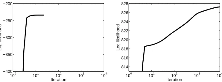
Figure 5: Example of training data log-likelihood convergence as a function of the number of EM iterations, for fluid-flow waveform data, comparing segmental HMMs (on the left) and random effects segmental HMMs (on the right), both using the EM algorithm, x-axis on a log-scale.

whereθ(t)is the estimate of the parameter vector from the previous M step of the tth EM iteration. P(si_r=k|yi_r,θ(t))in Equation (15) can be obtained from the F-B algorithm. The sufficient statistics, Ehui

r|sir=k,Y,θ(t)

i

and Ehui ruir

′

|si

r=k,Y,θ(t)

i

, for P(ui

r|sir=k,yir,θ(t)) in Equation (15) can be

directly obtained from Equations (9) and (10). The time complexity for an E step is O(M2T3N)

where N is the number of waveforms (and assuming each waveform is of length T ).

4.3.2 M STEP

In the M step, we find the values of the parameters that maximize Equation (14). As we can see from Equations (13a)-(13d) and (14), the optimization problem decouples into four parts, each of which involves a distinct set of parameters. Closed form solutions exist for all of the parameters

(the equations are included in Appendix A). The time complexity for each M step is O(MT3N).

In practice, the algorithm often converges relatively slowly, compared to segmental HMMs, due to the additional missing information in random effects parameters U. Figure 5 shows a typ-ical run of the algorithm. The segmental HMM converges much faster but converges to a lower log-likelihood value. The iterations were halted when the increase of the log-likelihood from one iteration to the next was less than 10−5.

Holmes and Russell (1999) augmented the observed waveform data with state sequences after

integrating out the random effects parameters, and used D_complete={Y,S}in the E step. In this

case the parameters for the segment distribution{β_k,σ2_,Ψ

k}do not decouple in the complete data

100 101 102 103 104 814

816 818 820 822 824 826 828

Iteration

Log likelihood

EM ECME

102 103 104 105 106

814 816 818 820 822 824 826 828

Time (sec)

Log likelihood

EM ECME

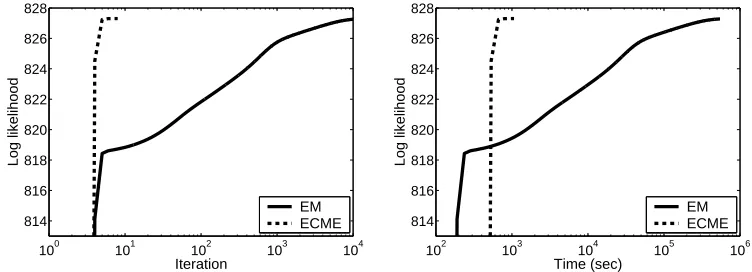
Figure 6: Example of training data log-likelihood convergence as a function of the number of it-erations (on the left) and as a function of computation time (on the right), for fluid-flow waveform data (the same data set as in Figure 5), comparing EM vs. ECME for the random effects segmental HMM, x-axis on a log-scale.

4.4 Faster Learning with ECME

As mentioned above, the convergence of the EM algorithm can be very slow especially in the es-timation of random effects models. Various extensions of the algorithm have been proposed to speed up the convergence. In the expectation conditional maximization (ECM) algorithm Meng

and Rubin (1993) replaced the M step of the EM algorithm with a sequence of W >1 constrained

or conditional maximizations (the CM steps). This does not necessarily decrease the number of EM iterations but can significantly reduce the total computation time. Liu and Rubin (1994) fur-ther extended the ECM algorithm to the ECME algorithm, reducing both the number of iterations and the total computation time. Both the ECM and the ECME algorithms preserve the property of monotone convergence of the EM algorithm.

More specifically, the CM step of the tth iteration of the ECM algorithm consists of W CM steps. The wth CM step maximizes Q(θ(t)_{,θ)under the constraint}

gw(θ) =gw(θ(t+(w−1)/W)),

where θ(t+w/W) denotes the value of θ in the wth CM step of the (t+1)th iteration and C=

{gw(θ),w=1, . . . ,W}is a set of W preselected vector functions. These constraints are set so that

the maximization is over the full parameter space ofθ. In a typical application of the ECM

algo-rithm the set of parametersθis divided into W subvectorsθ1, . . . ,θW and in the wth CM step of the

tth iteration Q(θ(t)_{,θ) is maximized overθ}

w. In this case gw(θ)is equal to θ−w, the vector of all

parameters except for θw. In all of the following discussion we assume gw(θ) has this particular

form.

−1 −0.9 −0.8 −0.7 −0.6 −5

0 5x 10

−3

Intercept

Slope

−2.6 −2.4 −2.2 −2 −1.8

0.032 0.033 0.034 0.035 0.036 0.037 0.038 Intercept Slope

15 20 25

−0.25 −0.2 −0.15

Intercept

Slope

State 1 State 2 State 3

−3 −2 −1 0 1

−0.015 −0.01 −0.005 0 Intercept Slope

−26 −24 −22 −20 −18

0.12 0.13 0.14 0.15 0.16 0.17 0.18 Intercept Slope

2.3 2.4 2.5 2.6 2.7

−8.5 −8 −7.5

−7x 10

−3

Intercept

Slope

State 4 State 5 State 6

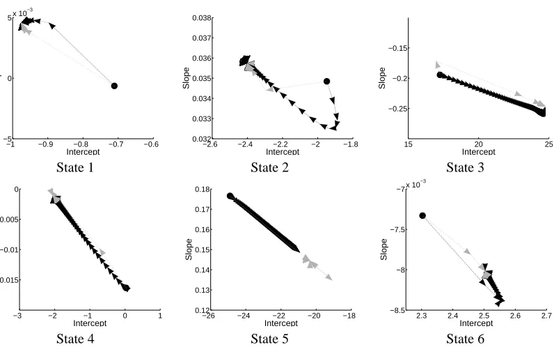
Figure 7: Convergence of β(x-axis is intercept, y-axis is slope) for fluid-flow data. The starting

point is indicated by a circle. Gray arrows represent ECME, black arrows represent EM. An arrow for the parameter values is drawn for each iteration in ECME and for every 100 iterations in EM.

Laird and Ware (1982) first derived an ECME algorithm for random effects models but mistak-enly thought it was the EM algorithm. Liu and Rubin (1994) gave a formal description of the ECME algorithm and introduced two different versions of the algorithm for random effects models. The first version has a closed form solution in the CM steps. The other requires an iterative algorithm for one of CM steps, and loses the monotone convergence property of the EM algorithm. Liu and Rubin report slightly faster convergence from the latter, but in our application of the ECME algorithm to random effects segmental HMMs we use the first version with closed form CM steps, thus, retaining the monotone convergence property of EM.

For random effects segmental HMMs we partition the parametersθintoθ1={A,Λ,Ψk,σ2|k=

1, . . . ,M} andθ2={βk|k=1, . . . ,M} and consider the ECME algorithm with two CM steps for

each of the two partitions as follows.

CM step 1: Compute A(t+1),Λ(t+1),Ψ_k(t+1), k=1, . . . ,M, and (σ2₎(t+1)_{as in the M step of the} EM algorithm.

CM step 2: GivenΨ(_kt+1), k=1, . . . ,M, and(σ2₎(t+1)_{obtained from CM Step 1, we can integrate}

out ui_{from Equations (13c)-(13d), and maximize∑}N

i=1∑R i

r=1log p(yir|βk,Ψ

(t+1)

k ,(σ2)(t+1),k=

si_r,di

r), where p(yir|βk,Ψ

(t+1)

k ,(σ2)(t+1),k=sir,dri)is given as

Nd(Xirβk,XirΨ

(t+1)

k X

i r ′

The update equations forβ(_kt+1), k=1, . . . ,M are

β(t+1)

k =

∑N

i=1∑t∑d<t Ciktd(Xitd

′

Zi tdXitd) P(yi_|θ(t)₎

−1

·

∑N

i=1∑t∑d<t Ciktd(Xitd

′

Zi tdytdi ) P(yi_|θ(t)₎

,

where X_tdi =X_ti_−d+1:t and

Zi_td= (Xi_tdΨ(_kt+1)X_tdi ′+ (σ2)(t+1)Id)−1.

When d is large we can avoid inverting a d×d matrix to obtain Zi_tdby rewriting this as

Zi_td={Id−Xitd((σ2)(t+1)(Ψk)−1+Xitd ′

Xi_td)−1Xi_td′}/(σ2₎(t+1)_.

CM step 1 maximizes the expected complete data log likelihood where both state sequences

S and random effects parameters U are considered missing. In CM step 2 the incomplete data

log likelihood is augmented only with S and then maximized. The computational complexity of the update equation forβ(_kt+1)in CM step 2 is O(MT4N)compared to O(MT3N)for the same parameter in the M step of the EM algorithm. Thus, the overall asymptotic complexity for the CM steps is

O(MT4_{N), and the ECME algorithm is computationally more expensive in time complexity per}

iteration than the EM algorithm.

The convergence of the EM and the ECME algorithms for a random effects segmental HMM with six states is shown in Figure 6 for the fluid-flow waveform data described in Section 5.1. The parameters were initialized to the same values for both algorithms and the convergence criterion

was set to 10−5. In Figure 6(a) the EM algorithm takes 11506 iterations to converge to roughly

the same log-likelihood that the ECME algorithm converges to in only 8 iterations. Each iteration takes 133.3s in the ECME algorithm, versus 47.4s in the EM algorithm, but the overall time to convergence of ECME is still over 3 orders of magnitude faster than EM (as shown in Figure 6(b)).

The convergence trajectories of the 2-dimensional parametersβ_kfor both algorithms are shown

in Figure 7 for each of the six states. The starting values are shown as black circles. Black arrows represent the parameter values of every 100 iterations in the EM algorithm and grey arrows represent the parameters in every iteration of the ECME algorithm. Both Figure 6 and Figure 7 show a dramatic improvement in the speed of convergence of ECME over EM: they both converge to the same solutions in parameter space but ECME converges much more quickly.

5. Experiments

We apply our model to two real-world data sets: (a) hot-film anemometry data in turbulent bubbly fluid-flow and (b) ECG heartbeat data: both are described in more detail below in Section 5.1. In all of our experiments we compare the results from our new segmental HMM with random effects to those obtained using segmental HMMs without random effects. We use several methods to evaluate the models:

50 100 150 200 250 −4 −3 −2 −1 0 1 2 3 time y (measurements)

50 100 150 200 250 −4 −3 −2 −1 0 1 2 3 time y (measurements)

50 100 150 200 250 −4 −3 −2 −1 0 1 2 3 time y (measurements)

50 100 150 200 250 −4 −3 −2 −1 0 1 2 3 time y (measurements)

(a) (b) (c) (d)

Figure 8: Negative examples in bubble-probe interaction data. (a) no interaction (b) glancing (c) bouncing (d) penetrating.

50 100 150 200 250 −2 −1 0 1 2 time y (measurements)

50 100 150 200 250 −2 −1 0 1 2 time y (measurements)

50 100 150 200 250 −2 −1 0 1 2 time y (measurements)

50 100 150 200 250 −2 −1 0 1 2 time y (measurements)

(a) (b) (c) (d)

Figure 9: Negative examples in ECG data (a) right bundle branch block beat (b) left bundle branch block beat (c) paced beat (d) premature ventricular contraction beat.

Segmentation Quality: To evaluate how well the model can segment test waveforms, we first

obtain the segmentations of test waveforms with the Viterbi algorithm, estimate the

regres-sion coefficients ˆγof each segment, and calculate the mean squared difference between the

observed data and Xˆγ. Good segmentations should produce low scores.

Recognition Accuracy: We use the model learned from a training set of positive examples to

recognize waveforms of interest from a test set with both positive and negative exemplars. We compare the results from random effects segmental HMMs with those from dynamic time warping (Keogh and Pazzani, 2000), Euclidean distance matching, and segmental HMMs.

All of the experiments were conducted using cross-validation. The number of segments M for each data set was determined by visual inspection prior to training the models. All waveforms were shifted to have zero mean amplitude before training and testing.

In all experiments reported below, we use the ECME algorithm for training random effects

segmental HMMs. The convergence criterion is set to 10−5. We found in our experiments that

providing one manually-segmented example is useful in initialization of both EM and ECME— details on initialization are described in Appendix B.

5.1 Data Sets

Bubble-probe ECG interaction data data

Avg. Avg. Avg. Avg.

LogP Segmentation LogP Segmentation Score Error Score Error

Segmental HMMs -3.25 15.39 -3.12 2.55

Random Effects Segmental HMMs 4.50 1.43 19.63 0.39

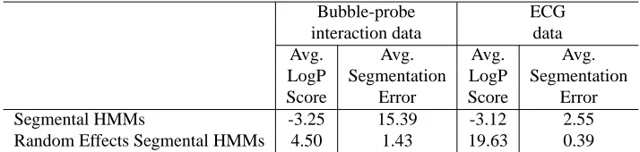
Table 1: Average logP scores and segmentation errors for bubble-probe interaction data and ECG data.

5.1.1 BUBBLE-PROBEINTERACTION DATA

Hot-film anemometry is a technique commonly used in turbulent bubbly flow measurements in fluid physics. Different types of interactions between the bubbles and the probe in turbulent gas flow, such as splitting, bouncing, and penetration, lead to characteristic waveform shapes. Automatically detecting the occurrence and types of interactions from such waveforms is a problem of active interest (Bruun, 1995). This recognition task is difficult because of the large variability in the shapes of waveforms within a given class of interactions (e.g., Figure 1(b)), caused by various factors such as velocity fluctuations and different gas fractions during measurement.

We applied our method to individual bubble-probe interaction data. Our data set consisted of 7 waveforms in the class no interaction (Figure 8(a)), 5 waveforms in the class glancing (Figure 8(b)), 52 waveforms in the class bouncing (Figure 8(c)), 8 waveforms in the class penetration (Figure 8(d)) and 48 waveforms in the class splitting (Figures 1(a) and (b)). Class labels were determined for each interaction based on expert examination of high-speed image recordings of the event obtained simul-taneously with the interaction signal (Luther, 2004). Each waveform had 256 data points sampled at 5kHz. We built waveform models for the class of splitting interactions, where the probe splits the bubble, and ran a 9-fold cross-validation with 5 waveforms in the training set and 43 waveforms in the test set for each run. The 72 waveforms from the other interactions were used as negative examples in the test set. Given that Figure 2(a) is a reasonable piecewise linear approximation of

the general shape, we subjectively chose M=6 as the number of states for both segmental HMMs

and random effects segmental HMMs.

5.1.2 ECG DATA

The shape of heartbeat cycles in ECG data can be used to diagnose the heart condition of a patient (Koski, 1996; Hughes et al., 2003). For example, Figure 11 shows the typical shape of normal heartbeats, whereas Figures 9(a)-(d) are taken from a heart experiencing various abnormal condi-tions. Heartbeats of the same type can vary significantly across individuals in terms of the heights and locations of peaks in the shape. Variability can also be found among heartbeats from the same individual although it is lower than across individuals.

For our experiments we used the ECG recordings with a sampling rate of 360 samples per

sec-ond from the MIT-BIH Arrhythmia database1. We selected hour long recordings from 23 subjects

and manually extracted two heartbeats of the same type from each subject. Normal heartbeats were

Top 10 Top 20

Euclidean distance (using mean distance) 86.7 81.7

Euclidean distance (using minimum distance) 82.2 80.0

Dynamic time warping (using mean distance) 85.6 82.2

Dynamic time warping (using minimum distance) 92.2 82.8

Segmental HMMs 86.7 82.2

Random Effects Segmental HMMs 100.0 95.0

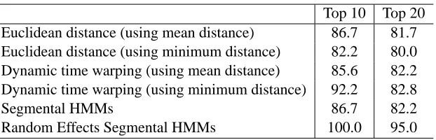
Table 2: Cross-validated recognition accuracy for bubble-probe interaction data on test set. The numbers represent the true positive rates in percentages (%) among the top k waveforms selected by each algorithm.

taken from each of twelve subjects, and similarly, left bundle branch block beats from three sub-jects, right bundle branch block beats from two subsub-jects, premature ventricular contraction beats from three subjects, and paced beats from three subjects. The lengths of heartbeats varied

approx-imately from 210 to 410 samples. We modeled each normal heartbeat with M=9 segments. We

performed a 4-fold cross-validation with 6 normal waveforms from three individuals as a training set for each cross-validation run and the remainder as a test set. Note that the test set contained heartbeats from a different set of individuals than the individuals used to train the model. Segmental HMMs could not be learned for one of the cross-validation runs due to numerical instability (a prob-lem that did not occur with random effects HMMs), so we report results from the remaining three runs of cross-validations for segmental HMMs. The 22 abnormal heartbeats were used as negative examples for the evaluation of recognition accuracy in the test sets.

5.2 Results

In Table 1 we compare the average logP scores of positive test waveforms for segmental HMMs with those for random effects segmental HMMs. The new model produces significantly higher scores for both data sets, indicating that random effects allow segmental HMMs to capture both the typical shape and shape variability.

Table 1 also shows the average segmentation errors for the test waveforms from both models. Adding the random effects component to segmental HMMs reduces the segmentation error roughly by a factor of 10 on both data sets. Segmentation examples are shown in Figure 10 for the bubble-probe interaction data and Figure 11 for the ECG data, where it is apparent that random effects segmental HMMs are more consistent in locating segment boundaries.

Rank Euclidean Dynamic time Segmental Random effects

distance warping HMM segmental HMM

1

2

3

4

5

6

7

8

9

10

0 50 100 150 200 250 −0.5

0 0.5 1 1.5 2

time

y (measurements)

0 50 100 150 200 250

−0.5 0 0.5 1 1.5 2

time

y (measurements)

Figure 11: Segmentation of a normal ECG heartbeat by the Viterbi algorithm for segmental HMMs (left) and for random effects segmental HMMs (right).

0 0.2 0.4 0.6 0.8 1

0 0.1 0.2 0.3 0.4 0.5 0.6 0.7 0.8 0.9 1

False positive rate

True positive rate

DTW − minimum distance DTW − mean distance Segmental HMM

Random effects segmental HMM

Figure 12: ROC plot for ECG data.

higher accuracy than any of the other methods. Figure 10 shows the top 10 waveforms found by the different methods. All of the false positives are from the interaction class bouncing, which is more similar in shape to the class splitting than other interaction types. Random effects segmental HMMs can effectively distinguish subtle differences in shape between the pattern that we are mod-eling and the non-pattern waveforms. Segmentations are overlaid in Figure 10 on the waveforms as found by probabilistic models using the Viterbi algorithm. Such segmentations are not available for dynamic time warping and Euclidean distance methods, providing an additional advantage of using probabilistic models in applications where segmentation is useful.

0 0.2 0.4 0.6 0.8 1 0

0.1 0.2 0.3 0.4 0.5 0.6 0.7 0.8 0.9 1

False positive rate

True positive rate

DTW − minimum distance DTW − mean distance Euclidean − minimum distance Euclidean − mean distance Segmental HMM

Random effects segmental HMM

Figure 13: ROC plot for bubble-probe interaction data.

6. Discussions and Conclusions

As noted elsewhere in the paper, the random effects segmental HMM proposed in this paper can be extended in multiple different ways. For example, the parametrization of the segment models as linear functions of time can be generalized directly to any functional form that is linear in the pa-rameters without altering the underlying time complexity of the learning and inference algorithms.

In the results reported here we applied our model to score relatively short waveform “snippets” to detect waveforms that are similar in shape to a query waveform. In order to parse online time-series data and detect “embedded” waveforms relative to a target, a two-state HMM with a pattern state and a background state can be used, where the random effects segmental HMM is embedded inside the pattern state. Each instance of the pattern waveform is allowed to have its own parameters via the random effects mechanism. The background state models any measurements that do not belong to pattern waveforms. A long time-series can then be parsed via the Viterbi algorithm (for example) to segment the series into background and pattern states, where the segments that belong to the pattern state correspond to predicted waveform locations according to the model.

In conclusion, we have proposed a probabilistic model that extends segmental HMMs to in-clude random effects. This model allows an individual waveform to vary its shape in a constrained manner via a prior distribution over individual waveform parameters. The ECME algorithm for learning this model greatly improved the speed of convergence of parameter estimation compared to a standard EM approach. Experimental results support the hypothesis that random effects seg-mental HMMs perform better in modeling, segmentation, and recognition of waveforms compared both to probabilistic models without random effects and to non-probabilistic methods.

Acknowledgments

Appendix A: Re-estimation Formulas for EM

The re-estimation formula for the transition probabilities and the duration distribution parameters can be shown to be:

a(_klt+1)=

∑N

i=1 1

P(yi_|θ(t)₎∑tα i t(k)a

(t)

klβ i∗ t (l)

∑N

i=1 1

P(yi_|θ(t)₎∑m∑tα i t(k)a

(t)

kmβ i∗ t (l)

,

λ(t+1)

k =

∑N

i=1 1

P(yi_|θ(t)₎∑t∑dCiktd·(d−1)

∑N

i=1 1

P(yi_|θ(t)₎∑t∑dCiktd

,

where

Ciktd=αit∗(k)P(d|λ

(t)

k )p(y i

t+1:t+d|θ

(t)

fk)β i t+d(k).

Using the notation of Xi_td=Xi_t−d+1:t and yi_td=yi_t−d+1:t, we update the covariance matrix of the top level of the segment distribution model according to

Ψ(t+1)

k =

∑N

i=1∑

t∑d<tCiktdE[uikuik

′

|Y,θ(t)]

P(yi_|θ(t)₎

∑N

i=1∑t∑d<t Ciktd P(yi_|θ(t)₎ ,

and for the bottom level, we re-estimate the parameters using

β(t+1)

k =

∑N

i=1

∑t∑d<tCiktd(Xitd

′

Xi td) P(yi_|θ(t)₎

−1

·

∑N

i=1

∑t∑d<tCiktd(Xtdi

′ (yi

td−XitdE[uik|Y,θ (t)

])

P(yi_|θ(t)₎

(σ2)(t+1)=

∑N

i=1

∑M

k=1∑t∑d<tCiktdE[Dik

′

Di k|Y,θ

(t)

]

P(yi_|θ(t)₎

∑N

i=1∑ M

k=1∑t∑d<tCiktdd P(yi_|θ(t)₎

,

where

E[Di_k′Di_k|Y,θ(t)] = (yi_t+1:t+d−Xi_tdβ_k−Xi_tdE[u_ki|Y,θ(t)])′·(yi_td−Xi_tdβ_k−Xi_tdE[u_ki|Y,θ(t)]) +tr[Xi_td′Xi_tdVar(ui_k|Y,θ(t))].

Appendix B: Initialization of the EM and ECME Algorithms

Given the manually segmented waveform, the parameters A,θd, andβk’s are set to their

maximum-likelihood values as estimated from this waveform. The 2×2 covariance matricesΨk’s of the

ran-dom effects component of the model require more than two segmented waveforms in order to obtain maximum-likelihood estimates—thus, their values are initialized in a different manner as follows. The variance term for the slope inΨk’s is set to a value generated from a uniform distribution over

[z_min,zmax]. From preliminary inspection of data zminand zmaxare set to 1 and 10 respectively for

bubble-probe interaction data, and 1 and 5 for ECG data. As the state index increases, the values of the intercept parameters inβ_k’s tend to increase and a small variability in slope leads to a more significant variability in intercept values. To take into account this we initialize the variance for

the intercept by sampling a value from the same uniform distribution[z_min,zmax]and multiplying

this value by the state index i for that intercept. Given that a positive change in the slope leads to a decreased value of the intercept we initialize the covariance between the slope and intercept to a negative value generated from a uniform distribution over[z_min×(−0.1),zmax×(−0.1)].

Multi-plying z_min and zmaxby 0.1 makes the covariance relatively small compared to variances inΨk’s

and also ensures that the covariance matricesΨk’s are positive definite. Finally, we sample the

ini-tial value for the noise parameterσ2from a uniform distribution over[1,6]for both data sets. This initialization strategy essentially sets the variance parametersΨk’s andσ2to relatively large initial

values and then lets them adjust to the training data.

References

Kannan Achan, Sam Roweis, Aaron Hertzmann, and Brendan Frey. A segment-based probabilistic generative model of speech. In Proc. of the 2005 IEEE International Conference on Acoustics, Speech, and Signal Processing, volume 5, pages 221–224, Philadelphia, PA, 2005. IEEE.

Rakesh Agrawal, Christos Faloutsos, and Arun N. Swami. Efficient similarity search in sequence databases. In Proc. of the 4th International Conference of Foundations of Data Organization and Algorithms, pages 69–84, Chicago, IL, 1993. Springer Verlag.

Theron Bennett and John Murphy. Analysis of seismic discrimination using regional data from western United States events. Bull. Seis. Soc. Am., 76:1069–1086, 1986.

Hans Bruun. Hot Wire Anemometry: Principles and Signal Analysis. Oxford University Press, Oxford, 1995.

King-pong Chan and Ada Wai-chee Fu. Efficient time series matching by wavelets. In Proc. of the 15th International Conference on Data Engineering, pages 126–133, Sydney, Australia, 1999. IEEE Computer Society.

Arthur Dempster, Nan Laird, and Donald Rubin. Maximum likelihood estimation from incomplete data via the EM algorithm. Journal of the Royal Statistical Society Series B, 39:1–38, 1977.

Arthur Dempster, Donald Rubin, and Robert Tsutakawa. Estimation in covariance components models. Journal of the American Statistical Association, 76(374):341–353, 1981.

James Ferguson. Variable duration models for speech. In Proc. of the Symposium on the Application of Hidden Markov Models to Text and Speech, pages 143–179, Princeton, NJ, 1980. IDA-CRD.

Mark Gales and Steve Young. The theory of segmental hidden Markov models. Technical Report CUED/F-INFENG/TR 133, Cambridge University Engineering Department, 1993.

Xianping Ge and Padhraic Smyth. Deformable Markov model templates for time-series pattern matching. In Proc. of the 6th ACM SIGKDD International Conference on Knowledge Discovery and Data Mining, pages 81–90, Boston, MA, 2000. ACM Press.

Wendy Holmes and Martin Russell. Probabilistic-trajectory segmental HMMs. Computer Speech and Language, 13(1):3–37, 1999.

Nicholas Hughes, Lionel Tarassenko, and Stephen Roberts. Markov models for automated ECG interval analysis. In Advances in Neural Information Processing Systems 16, pages 611–618, Cambridge, MA, 2003. MIT Press.

Stanislaw Jankowski and Artur Oreziak. Learning system for computer-aided ECG analysis based on support vector machines. International Journal of Bioelectromagnetism, 5(1):175–176, 2003.

Michael Jordan, editor. Learning in Graphical Models. MIT Press, Cambridge, MA, 1999.

Eamonn Keogh and Michael Pazzani. Scaling up dynamic time warping for datamining applications. In Proc. of the 6th ACM SIGKDD International Conference on Knowledge Discovery and Data Mining, pages 285–289, Boston, MA, 2000. ACM Press.

Eamonn Keogh and Padhraic Smyth. A probabilistic approach to fast pattern matching in time series databases. In Proc. of the 3rd ACM SIGKDD International Conference on Knowledge Discovery and Data Mining, pages 24–30, Newport Beach, CA, 1997. AAAI Press.

Seyoung Kim, Padhraic Smyth, and Stefan Luther. Modeling waveform shapes with random effects segmental hidden Markov models. In Proc. of the 20th International Conference on Uncertainty in AI, pages 309–316, Banff, Canada, 2004. AUAI Press.

Antti Koski. Modelling ECG signals with hidden Markov models. Artificial Intelligence in

Medicine, 8(5):453–471, 1996.

Nan Laird and James Ware. Random-effects models for longitudinal data. Biometrics, 38(4):963– 974, 1982.

Nan Laird, Nicholas Lange, and Daniel Stram. Maximum likelihood computations with repeated measures: application of the EM algorithm. Journal of the American Statistical Association, 82 (397):97–105, 1987.

Stephen Levinson. Continuously variable duration hidden Markov models for automatic speech recognition. Computer Speech and Language, 1(1):29–45, 1986.

Chuanhai. Liu and Donald Rubin. The ECME algorithm: a simple extension of EM and ECM with faster monotone convergence. Biometrika, 81(4):633–648, 1994.

Xiao-Li Meng and Donald Rubin. Maximum likelihood estimation via the ECM algorithm: a general framework. Biometrika, 80:267–278, 1993.

Carl Mitchell, Mary Harper, and Leah Jamieson. On the computational complexity of explicit duration HMMs. IEEE Trans. on Speech and Audio Processing, 3(3):213–217, 1995.

Kevin Murphy. Dynamic Bayesian Networks: Representation, Inference, and Learning. PhD thesis, University of California, Berkeley, 2002.

Mari Ostendorf, Vassilios Digalakis, and Owen Kimball. From HMMs to segmental models: a unified view of stochastic modeling for speech recognition. IEEE Trans. on Speech and Audio Processing, 4(5):360–378, 1996.

Lawrence Rabiner and Biing-Hwang Juang. Fundamentals of Speech Recognition. Prentice Hall, Englewood Cliffs, NJ, 1993.

Martin Russell. A segmental HMM for speech pattern matching. In Proc. of the 1993 IEEE Inter-national Conference on Acoustics, Speech and Signal Processing, pages 499–502, Minneapolis, MN, 1993. IEEE.

Martin Russell and Roger Moore. Explicit modeling of state occupancy in hidden Markov mod-els for automatic speech recognition. In Proc. of the 1985 IEEE International Conference on Acoustics, Speech and Signal Processing, pages 2376–2379, Tampa, FL, 1985. IEEE.

Shayle Searle, George Casella, and Charles McCulloch. Variance Components. Wiley, New York, 1992.

Yair Shimshoni and Nathan Intrator. Classification of seismic signals by integrating ensembles of neural networks. IEEE Trans. on Signal Processing, 46:1194–1201, 1998.

Byoung-Kee Yi and Christos Faloutsos. Fast time sequence indexing for arbitrary Lp norms. In

Proc. of the 26th Very Large Data Bases Conference, pages 385–394, Cairo, Egypt, 2000. Morgan Kaufmann.