Stabilized Sparse Online Learning for Sparse Data
Yuting Ma [email protected]
Department of Statistics Columbia University New York, NY, USA
Tian Zheng [email protected]
Department of Statistics Columbia University New York, NY, USA
Editor:Sathiya Keerthi
Abstract
Stochastic gradient descent (SGD) is commonly used for optimization in large-scale machine learning problems. Langford et al. (2009) introduce a sparse online learning method to induce sparsity via truncated gradient. With high-dimensional sparse data, however, this method suffers from slow convergence and high variance due to heterogeneity in feature sparsity. To mitigate this issue, we introduce a stabilized truncated stochastic gradient descent algorithm. We employ a soft-thresholding scheme on the weight vector where the imposed shrinkage is adaptive to the amount of information available in each feature. The variability in the resulted sparse weight vector is further controlled by stability selection integrated with the informative truncation. To facilitate better convergence, we adopt an annealing strategy on the truncation rate, which leads to a balanced trade-off between exploration and exploitation in learning a sparse weight vector. Numerical experiments show that our algorithm compares favorably with the original truncated gradient SGD in terms of prediction accuracy, achieving both better sparsity and stability.
Keywords: sparse online learning, sparse features, truncated gradient, stability selection, adaptive shrinkage
1. Introduction
Modern data sets pose many challenges for existing learning algorithms due to their unprecedented large scales in both sample sizes and input dimensions. It demands both efficient processing of massive data and effective extraction of crucial information from an enormous pool of heteroge-neous features. In response to these challenges, a promising approach is to exploit online learning methodologies that performs incremental learning over the training samples in a sequential manner. In an online learning algorithm, one sample instance is processed at a time to obtain a simple update, and the process is repeated via multiple passes over the entire training set. In comparison with batch learning algorithms in which all sample points are scrutinized at every single step, online learning algorithms have been shown to be more efficient and scalable for data of large size that cannot fit into the limited memory of a single computer. As a result, online learning algorithms have been widely adopted for solving large-scale machine learning tasks (e.g., Bottou, 1998).
c
In this paper, we focus on first-order subgradient-based online learning algorithms, which have been studied extensively in the literature for dense data.1Among these algorithms, popular methods include the Stochastic Gradient Descent (SGD) algorithm in (Zhang, 2004) and (Bottou, 2010), the mirror descent algorithm introduced by Beck and Teboulle (2003) and the dual averaging algorithm by Nesterov (2009). Since these methods only require the computation of a (sub)gradient for each incoming sample, they can be scaled efficiently to high-dimensional inputs by taking advantage of the finiteness of the training sample. In particular, the stochastic gradient descent algorithm is the most commonly used algorithm in the literature of subgradient-based online learning. It enjoys an exceptionally low computational complexity while attaining steady convergence under mild conditions as discussed in (Bottou, 1998), even for cases where the loss function is not everywhere differentiable.
Despite of their computational efficiency, online learning algorithms without further constraint on the parameter space suffers the “curse of dimensionality” to the same extent as their non-online counterparts. Embedded in a dense high-dimensional parameter space, not only does the resulted model lack interpretability, its variance is also inflated. As a solution,sparse online learningwas introduced to induce sparsity in the parameter space under the online learning framework (e.g., Langford et al., 2009). It aims at learning a linear classifier with a sparse weight vector, which has been an active topic in this area. For most efforts in the literature, sparsity is introduced by applying L1 regularization on a loss function, such as in (Shalev-Shwartz and Tewari, 2011), in
the same fashion as in the classific LASSO method by Tibshirani (1996). For example, Duchi and Singer (2009) extend the framework of Forward-Backward splitting method introduced by Lions and Mercier (1979) which alternates between an unconstrained truncation step on the sample gradi-ent and an optimization step on the loss function with a penalty on the distance from the truncated weight vector.Langford et al. (2009) and Carpenter (2008) both explore the idea of imposing a soft-thresholdon the weight vectorw∈Rpupdated by the stochastic gradient descent algorithm:
wj =sign(wj) max(|wj| −λ,0), j= 1, . . . , p.
This class of methods is known as thetruncated gradient algorithm. For everyK standard SGD updates, the weight vector is shrunk by a fixed amount to induce sparsity. In (Duchi et al., 2010), the same strategy has also been combined with a variant of the mirror descent algorithm in (Beck and Teboulle, 2003). Wang et al. (2015) further extends the truncated gradient framework to adjust for cost-effectiveness. This simple yet efficient method of truncated gradients particularly motivates the algorithm proposed in this paper. Strategies different from the truncation-based algorithm have also been proposed. For example, Xiao (2009) proposed the Regularized Dual-Averaging (RDA) algorithm which builds upon the primal-dual subgradient method by Nesterov (2009). The RDA algorithm learns a sparse weight vector by solving an optimization problem using the running average over all preceding gradients, instead of a single gradient at each iteration.
Closely related to sparse online learning is another area of active research, online feature se-lection. Instead of enforcing just a shrinkage on the weight vectors viaL1 regularization, online
feature selection algorithms explicitly invoke feature selection by imposing a hardL0constraint on
the weight vector, (e.g., Wang et al., 2014; Wu et al., 2014). In other words, online feature selection algorithms focus on generating a resulted weight vector that has a high sparsity level by directly
shrinking a large proportion of the weights directly to zero (also referred to as ahard thresholding). In practice,L0regularization is computationally expensive to solve due to its non-differentiability.
The set of selected features also suffers from high variability as the decisions of hard-thresholding are based on single random samples in an online learning setting. Therefore, important features can be discarded simply owing to random perturbations.
Most recent subgradient-based online learning algorithms do not consider potential structures or heterogeneity in the input features. As pointed out by Duchi et al. (2011), current methods largely follow a predetermined procedural scheme that is oblivious to the characteristics of data being used at each iteration. In large-scale applications, a common and important structure is heterogeneity in sparsity levels of the input features, i.e., the variability in the number of nonzero entries among features. For instance, consider the bag-of-word features in text mining applications.2 For a learning task, the importance of a feature is not necessarily associated with the frequencies of its values. In genetics, for example in (Morris and Zeggini, 2010), rare variants (≤ 1% in the population) have been found to be associated with disease risks. Both dense and sparse features may contain important information for the learning task. However, in the presence of heterogeneity in sparsity levels, using a simple L1 regularization in an online setting will predispose rare features to be
truncated more than necessary. The resulted sparse weight vectors usually exhibit high variance in terms of both weight values and the membership in the set of features with nonzero weights. As a result, the convergence of the standard truncation-based framework may also be hampered by this high variability. When the amount of information is scarce due to sparsity at each iteration, the convergence of the weight vector would understandably take a large number of iterations to approach the optimum. In two recent papers, Oiwa et al. (2011) and Oiwa et al. (2012) tackle this problem via L1 penalty weighted by the accumulated norm of subgradients for extending
several basic frameworks in sparse online learning. Their results suggest that, by acknowledging the sparsity structure in the features, both prediction accuracy and sparsity are improved over the original algorithms while maintaining the same convergence rate. However, their resulted weight vectors are unstable as the imposed subgradient-based regularization are excessively noisy due to the randomness of incoming samples in online learning. The membership in the set of selected features with nonzero weights is also very sensitive to the orderings of the training samples.
In this paper, we propose astabilized truncated stochastic gradient descentalgorithm for high-dimensional sparse data. The learning framework is motivated by that of the Truncated Gradient algorithm proposed by Langford et al. (2009). To deal with the aforementioned issues with sparse online learning methods applied to high-dimensional sparse data, we introduce three innovative components to reduce variability in the learned weight vector and stabilize the selected features. First, when applying the soft-thresholding, instead of a uniform truncation on all features, we perform onlyinformative truncations, based on actual information from individual features during the preceding computation window of K updates. By doing so, we reduce the heterogeneous truncation bias associated with feature sparsity. The key idea here is to ensure that each truncation for each feature is based on sufficient information, and the amount of shrinkage is adjusted for the information available on each feature. Second, beyond the soft-thresholding corresponding to the ordinary L1 regularization, the resulted weight vector isstabilized by staged purges of irrelevant
features permanently from the active set of features. Here, irrelevant featuresare defined as fea-tures whose weights have been repeatedly truncated. Motivated by stability selection introduced
by Meinshausen and B¨uhlmann (2010), these permanent purges prevent irrelevant features from oscillating between the active and non-active set of features, The “purging” process also resembles hard-thresholding in online feature selection and results in a stabler sparse solution than other sparse online learning algorithms. Results on the theoretical regret bound (See Section 4) show that this stabilization step helps improve over the original truncated gradient algorithm, especially when the target weight vector is notably sparse. To attune the proposed learning algorithm to the sparsity of the remaining active features, the third component of our algorithm is adjusting the amount of shrinkage progressively instead of fixing it at a predetermined value across all stages of the learning process. A novel hyperparameter, rejection rate, is introduced to balance between exploration of different sparse combinations of features at the beginning and the exploitationof the selected features to construct accurate estimate at a later stage. Our method gradually anneal the rejection rate to acquire the necessary amount of shrinkage on the fly for achieving the desired balance.
The rest of paper is organized as follows. Section 2 reviews the Truncated Gradient algorithm based on Stochastic Gradient Descent (SGD) framework for sparse learning proposed by Langford et al. (2009). In Section 3, we introduce, in details, the three novel components of our proposed algorithm. Theoretical analysis of the expected online regret bound is given in Section 4, along with the computational complexity. Section 5 gives practical remarks for efficient implementation. In Section 6, we evaluate the performance of the proposed algorithm on several real-world high-dimensional data sets with varying sparsity levels. We illustrate that the proposed method leads to improved stability and prediction performance for both sparse and dense data, with the most improvement observed in data with the highest average sparsity level. Section 7 concludes with further discussion on the proposed algorithm.
2. Truncated Stochastic Gradient Descent for Sparse Learning
Assume that we have a set of training dataD = {zi = (xi, yi), i = 1, . . . , n}, where the feature vectorxi ∈Rpand the scalar outputyi ∈R. In the following, we usexi to represent the vector of theithsample of lengthpandx·,jfor thejthfeature vector of all samples of lengthn. In this paper, we are interested in the case that bothpandnare large and the feature vectorsx·,j’s,j = 1, . . . , p, are sparse. We consider a loss functionl(ˆy, y)that measures the cost of predictingyˆwhen the truth isy. The predictionyˆis given by functionfw(x)from a familyFparametrized by a weight vector
w. DenoteL(w,z)==def l(fw(x), y). The learning goal is to obtain an optimal weight vectorwˆ that
minimize the loss function n
P
i=1
L(w, zi) over the training data, with sparsity in the weight vector
induced by a regularization termΨ(w). We can then formulate the learning task as a regularized minimization problem:
ˆ
w= arg min
w∈Rp
n
X
i=1
L(w, zi) + Ψ(w). (1)
based on subsets of the training data. This is particularly attractive to large scale problems as it leads to a substantial reduction in computing complexity and potentially distributed implementation.
For applications with large data sets or streaming data feeds, SGD has also been used as a subgradient-basedonline learningmethod. Cesa-Bianchi et al. (2004) argue that online learning and stochastic optimization are closely related and interchangeable most of the time. For simplicity, in the following, we focus our discussion and algorithmic description under the online learning frame-work with regret bound models. Nonetheless, our results can be readily generalized to stochastic optimization as well.
In online learning, the algorithm receives a training sample zt = (xt, yt) at a time from a continuous feed. Without sparsity regularization, at timet, the weight vector is updated in an online fashion with a single training samplezt∈ Ddrawn randomly
wt=wt−1−ηL0(wt−1, zt), (2)
whereη >0is the learning rate andL0(wt, zt)∈∂wtL(wt, zt)is a subgradient of the loss function
L(wt, zt)with respect towt. The set of subgradients of f at the pointxis called the subdifferential off atx, and is denoted∂f(x). A functionf is called subdifferentiable if it is subdifferentiable at allx ∈domf. When L(w,·)is differentiable atw,∂wL(w,·) = {∇wL(w,·)}. At the same time, a sequence of decisions wt is generated at t = 1,2, . . ., that encounters a loss L(wt, zt) respectively.
The goal of online learning algorithm with sparsity regularization is to achievelowregret with respect to a fixed optimal weight vectorw∗ ∈ W ⊂Rp. Here,Wis the parameter space for sparse weights vectors (see Assumption 3 on page 15 for more details.) The regret is defined as:
RT(w∗), T
X
t=1
(L(wt, zt) + Ψ(wt))− T
X
t=1
(L(w∗, zt) + Ψ(w∗)). (3)
In this paper, we focus on theL1regularization whereΨ(w) =g||w||1andgis the regularizing
parameter. When adopted in an online learning framework, standard SGD algorithm does not work well in addressing (1) withL1 penalty. Firstly, a simple online update requires the projection of
the weight vectorwonto a L1-ball at each step, which is computationally expensive with a large
number of features. Secondly, with noisy approximate subgradient computed using a single sample, the weights can easily deviate from zero due to the random fluctuations inzt’s. Such a scheme is therefore inefficient to maintain a sufficiently sparse weight vector.
To address this issue, Langford et al. (2009) induced sparsity inwby subjecting the stochastic gradient descent algorithm to soft-thresholding. For everyK ∈ N+ iterations at step t, each of
which is as defined in (2), the weight vector is shrunk by a soft-threshold operatorT with agravity parameterg ∈ G ⊂Rp withg
j ≥0forj = 1, . . . , p. For a vectorw= [w1, . . . , wp]∈Rp,
ˆ
wt=T(wt,g), (4)
whereT(w,g) = [T(w1, g1), . . . , T(wp, gp)]with the operatorT defined by
T(wj, gj),
max(wj−gj,0), ifwj >0;
Algorithm 1 B0(w0, g0): A burst of K updates with truncation using a universal gravity as in
truncated SGD by Langford et al. (2009).
Input:w0at initialization and the base gravityg0. Parameters: K,η.
fort= 1toKdo
Drawzt∈ Duniformly at random.
wt=wt−1−ηL0(wt−1, zt), whereL0(wt−1, zt)∈∂wt−1L(wt−1, zt). end for
ˆ
w=T(wK, g0K1p).
Return: wˆ.
As one can see, the sequence ofK SGD updates can be treated as a unit computational block, which will be referred to as abursthereafter. Here the wordburstindicates that it is a sequence of repetitive actions, e.g., the standard SGD updates as defined in (2), without interruption. Each burst is followed by asoft-thresholding truncationdefined in (4), which puts a shrinkage on the learned weight vector.
A burst can be viewed as a base feature selection realized on a set of random samples withL1
regularization as in the classical LASSO by Tibshirani (1996). Within a burst, letXKbe the set of
K random samples on which the weight vector wˆ is stochastically learned. We define the set of features with nonzero weights inwˆ as itsactive (feature) set:
ˆ
Sg( ˆw;X
K) ={j :|wˆj|>0}, (6)
with a corresponding gravityg. The steps within a truncated burst are summarized in Algorithm 1. In the truncated gradient algorithm, the gravity parameter is a constant across all dimensions as
g =g0K1p, whereg0 ∈R≥0is abase gravityfor each update in a burst and1p ,(1, . . . ,1)∈
Rp. In general, with greater parameterg0and smaller burst sizeK, more sparsity is attained. When g0= 0, the update in (4) becomes identical to the standard stochastic gradient descent update in (2).
Langford et al. (2009) showed that this updating process can be regarded as an online counterpart ofL1regularization in the sense that it approximately solves (1) in the limit asK → ∞andη→0.
3. Stabilized Truncated SGD for Sparse Learning
Truncated SGD works well for dense data. When it comes to high-dimensional sparse inputs, however, it suffers from a number of issues. Shalev-Shwartz and Tewari (2011) observe that the truncated gradient algorithm is incapable of maintaining sparsity of the weight vector as it iterates. Recall that, under the online learning setting, the weight vectorwis updated with a noisy approximation of the true expected gradient using one sample at a time, from a random ordering of the data. With sparse inputs, it is highly probable that an important feature does not have a nonzero entry for many consequent samples, and is meaningfully updated for only a few times out of the
0 200 400 600 800 1000
0
10
20
30
40
Iteration
% Nonz
ero V
ar
iab
les
Truncated Gradient:Truncation Stabilized Truncated SGD:Truncation Ordinary SGD Update
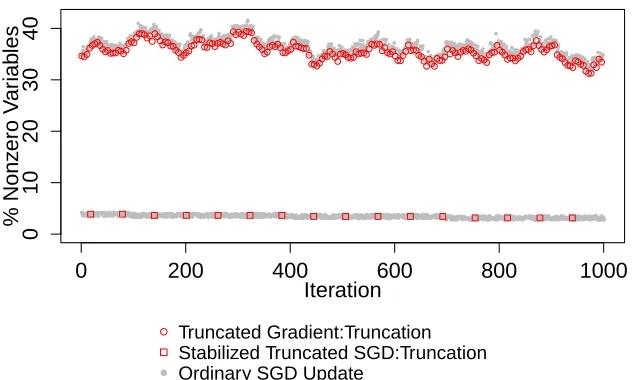
Figure 1: An example of the truncated SGD algorithm by Langford et al. (2009) and the proposed stabilized truncated SGD algorithm applied to a high-dimensional sparse data set. Here we compare the percentage of nonzero variables in the resulted weight vector at each iteration during the last 1000 iterations of both algorithms. The underlying data set is the text mining data set, Dexter, with 10,000features and 0.48% of sparsity, which is described in details in Section 6.
1000 stochastic updates from the truncated gradient algorithm implemented on a high-dimensional sparse data set are shown in Figure 13. It can be seen that the numbers of nonzero features in the weight vectors learned by the truncated SGD algorithm (K = 5) remain large and highly unstable throughout these 1000 iterations, oscillating within 10% of the total number of features. As a comparison, also in Figure 1, we plot the results from our proposed stabilized truncated SGD applied to the same data. During these last 1000 updates, the proposed algorithm is using a less frequent truncation schedule due to ourannealed reject rate. It attains both high sparsity in the weight vector and high stability with high-dimensional sparse data.
In this section, we introduce the stabilized truncated Stochastic Gradient Descent (SGD) al-gorithm. It attains a truly sparse weight vector that is stable and gives generalizable performance. Our proposed method attunes to the sparsity of each feature and adoptsinformative truncation. The algorithm keeps track of whether individual features have had enough information to be confidently subject to soft-thresholding. Based on the truncation results, we systematically reduce the active feature set by permanently discarding features that are truncated to zero with high probability via stability selection. We further improve the efficiency of our algorithm by adapting gravity to the sparsity of the current active feature set as the algorithm proceeds.
3.1 Informative Truncation
In the truncated SGD algorithm, Langford et al. (2009) suggest a general guideline for determining gravity in the batch mode by scaling a base gravityg0 by K, the number of updates, for a single
truncation after a burst. A direct online adaptation of aL1regularization would shrinks the weight
vector at every iteration. The above batch mode operation is to delay the shrinkage forKiterations so that the truncation is executed based on information collected fromK random samples instead of from a single instance. This guideline implicitly assumes that theKSGD updates in a burst are equally informative, which is in general true for dense features. For sparse features, however, under the online learning setting, not every update is informative about every feature due to the scarcity of nonzero entries. The original uniform formula,g = Kg01p, for gravity would then create an undesirable differential treatment for features with different levels of sparsity. With a relatively small K, it is very likely that a substantial proportion of features would have no non-zero values on a size-Ksubsample used in a particular burst. The weights for these features remain unchanged after K updates. Consequently, the set of sparse features run the risk of being truncated to zero based on very few informative updates. The truncation decision is therefore mostly determined by a feature’s sparsity level, rather than its relevance to the class boundary.
To make the learning be informed of the heterogeneity in sparsity level among features, we introduce the informative truncationstep, extended from the idea of base gradient used in Algo-rithm 1. Instead of applying a universal gravity proportional to K to all features, the amount of shrinkage is set proportional to the number of times that a feature is actually updated with nonzero values in the size-K subsample, i.e., the number ofinformative updates. Specifically, within each burst, the algorithm keeps a vector ofcounters,k˜ ∈Rp, of the numbers of informative updates for the featuresx·,j,j = 1, . . . , p. Letg0 ∈ R ≥ 0 be the base gravity parameter that serves as the
unit amount of shrinkage for each informative update on each feature. At the end of each burst, we shrink feature x·,j by g0˜kj. In other words, here we setg = g0k˜. The computational steps for a
burst with informative truncation in summarized in Algorithm 2.
Algorithm 2B1(w0, g0): A burst ofKupdates with informative truncation. Input:w0at initialization and the base gravityg0.
Initialization: k˜=0p ∈Rp. Parameters: K,η.
fort= 1toKdo
Drawzt= (xt, yt)∈ Duniformly at random.
wt=wt−1−ηL0(wt−1, zt), whereL0(wt−1, zt)∈∂wt−1L(wt−1, zt).
˜
k←k˜+I(|xt|>0).
end for
ˆ
w=T(wK, g0k˜). Return: wˆ,k˜.
to the truncated gradient algorithm that quickly shrinks many features to zero indiscriminately, informative truncation keeps sparse features until enough evaluation is conducted. In doing so, sparse yet important features will be retained. The proposed approach also reduce the variability in the resulted sparse weight vector during the training process. Duchi et al. (2011) use a similar strategy that allows the learning algorithm to adaptively adjust its learning rates for different features based on cumulative update history. They use theL2norm of accumulated gradients to regulate the
learning rate. By adapting the gravity with the counterk˜ within each burst, our proposed strategy here can be viewed as applying theL0 norm to the accumulated gradients that is refreshed everyK
steps.
3.2 Stability Selection
Despite of its scalability, subgradient-based online learning algorithms commonly suffer from in-stability. It has been shown both theoretically and empirically that stochastic gradient descent algorithms are sensitive to random perturbations in training data as well as specifications of learning rate (e.g., Toulis et al., 2015; Hardt et al., 2015). This instability is particularly pronounced in sparse online learning with sparse data, as discussed in Section 1. Under an online learning setting, using random ordering of the training sample as inputs, the algorithm would produce distinct weight vectors and unstable memberships of the final active feature set. Moreover, there has been a lot of discussion on the link between the instability of an learning algorithm and its deteriorated general-izability in the literature (e.g., Bousquet and Elisseeff, 2002; Kutin and Niyogi, 2002; Rakhlin et al., 2005; Shalev-Shwartz et al., 2010).
To tackle this instability issue, in the proposed algorithm, we exploit the method of stability selectionto improve its robustness to random perturbation in the training data. Stability selection by Meinshausen and B¨uhlmann (2010) does not launch a new feature selection method. Rather, its aim is to enhance and improve a sparse learning method via subsampling. The key idea of stability se-lection is similar to the generic bootstrap. It feeds the base feature sese-lection procedure with multiple random subsamples to derive an empirical selection probability. Based on aggregated results from subsamples, a subset of features is selected with low variability across different subsamples. With proven consistency in variable selection, stability selection helps remove noisy irrelevant features and thus reduce the variability in learning a sparse weight vector.
Incorporating stability selection into our proposed framework, each truncated burst with gravity parameter g is treated as an individual sparse learning engine. It takes K random samples and carries out a feature selection to obtain a sparse weight vector. In the following, we define first the notion ofselection probabilityfor the stability selection step in our proposed algorithm.
Definition 1 (selection probability) LetXKbe a random subsample of{1, . . . , n}of sizeK, drawn
without placement. Parametrized by the gravity parameterg, the probability of the featurex·,jbeing
in the active set of a truncated burst that returnswˆ is
Πgj =P∗
j ∈Sˆg( ˆw;XK)
=ED[I(|wˆj|>0)],
where the probabilityP∗is with respect to the random subsampling ofXK. LetΠg = [Πg1, . . . ,Π
g p].
Under unknown data distribution, the selection probabilities cannot be computed explicitly. Instead, they are estimated empirically. Since each truncation burst performs a screening on all features, the frequency of each feature being selected by a sequence of bursts can be used to derive an estimator of the selection probability. We denote a sequence ofnK > 0 truncated bursts as a
stage. A preliminary empirical estimate of the selection probability is given by
ˆ Πj =
P
τ:˜kj,τ >0I(|wˆj,τ|>0) nk
P
τ=1
I(˜kj,τ>0)
, forjs.t. nK
P
τ=1
˜
kj,τ >0;
1, otherwise,
(7)
wherek˜τ are the counters of informative updates for burstτ,τ = 1, . . . , nK.
Different from the conventional stability selection setting, wˆτ’s are obtained sequentially and thus are dependent with each other. When nK is small, different subsamples produce selection probability estimates using (7) exhibit high variability, even when initialized with the same weight vector atτ = 1. On the other hand, a large value ofnK requires a prohibitively large number of iterations for convergence. To resolve the issues of estimating selection probability using a single sequence of SGD updates, we introduce a multi-thread framework of updating paths. Multiple threads of sequential SGD updates are executed in a distributed fashion, which readily utilizes modern multi-core computer architecture. WithM processors, we initialize the algorithm on each path of SGD updates with a random permutation of the training data,D, denoted asD(1), . . . ,D(m).
Then independently, M stages of bursts run in parallel along M paths, which return withwˆ(τm),
τ = 1, . . . , nK, m = 1, . . . , M. The joint estimate of selection probability with gravity g is obtained as
ˆ Πj =
M P m=1 P
τ:˜k(j,τm)>0I(|wˆ
(m)
j,τ |>0) M P m=1 nk P τ=1
I(˜kj,τ(m)>0)
, forjs.t. M P m=1 nK P τ=1 ˜
k(j,τm) >0;
1, otherwise.
(8)
When more processors are available, a smallernKis required for the algorithm to obtain a stable estimate of selection probability. The dependence amongwˆτ’s is also attenuated whenM random subsets of samples are used for the estimation. This strategy falls under parallelized stochastic gradient descent methods, which is discussed in detail by Zinkevich et al. (2010).
Under the framework of stability selection, each stage on every path uses a random subsample. The estimated selection probability quantifies the chance that a feature is found to have high rele-vance to class differences given a random subsample. At the end of each stage,stable featuresare identified as those that belong to a large fraction of active sets incurred during this stage of bursts.
Definition 2 (Stable Features) For a purging thresholdπ0 ∈ [0,1], the set of stable features with gravity parametergis defined as
ˆ
Ωg ={j: Πgj ≥π0}. (9)
For simplicity, we write the stable setΩˆg asΩˆ when there is no ambiguity.
Algorithm 3B2(w0, g0,Ωˆ,D(m)): Informative truncated burst with stability selection in threadm. Input: w0,g0, the input dataD(m) and the current set of stable featuresΩˆ, which is the output
of equation (9) using (8) with predetermined thresholdπ0. Parameters: K,η.
Initializev0= (w0,j)j∈Ωˆ ,k˜=0|Ωˆ|. fort= 1toKdo
Drawzt= (xt, yt)sequentially fromD(m). ˜
zt= (zt,j)j∈Ωˆ.
vt=vt−1−ηL0(vt−1,z˜t), , whereL0(vt−1, zt)∈∂vt−1L(vt−1, zt).
˜
k←k˜+I(|xt|>0).
end for
ˆ
u=T(vK, g0k˜).
ˆ
wj =
ˆ
uj0, ifj∈Ωˆ andΩˆj0 =j;
0, ifj /∈Ωˆ. Return: wˆ,k˜.
the set of stable features by permanently setting their corresponding weights to zero, and remove them from subsequent updates. We define thestabilizedweight vector as
˜
w= ˆw·IΩˆ. (10)
As discussed above, due to the nature of online learning with sparse data, there are two unde-sirable learning setbacks in a single truncated burst. The first occurs when an important feature has its weight stuck at zero due to inadequate information in the subsample used, while the second case is when a noise feature’s weight gets sporadic large updates by chance. Using informative bursts, we can avert the first type of setbacks and using selection probability based on multiple bursts, we can spot noisy features more easily. In the presence of a large number of noisy features, the learned weights for important features suffer from high variance. Via stability selection, we systematically remove noisy features permanently from the feature pool. Furthermore, the choice of a proper regularization parameter is crucial yet known to be difficult for sparse learning, especially due to the unknown noise level. Applying stability selection renders the algorithm less sensitive to choice of the base gravity parameterg0 in learning a sparse weight vector via truncated gradient. As we
will show using results from our numerical experiments, this purging by stability selection leads to a notable reduction in the estimation variance of the weight vector. Here,π0 is a tuning parameter
in practice. We have found that the learning results in the numerical experiments are not sensitive to different values ofπ0within a reasonable range. Under mild assumptions discussed in Section 4, we
derive a lower bound of the expected improvement in convergence by employing stability selection in the learning process in Lemma 2.
3.3 Adaptive Gravity with Annealed Rejection Rate
The truncated SGD algorithm adopts a universal and fixed base gravity parameter at all truncations. As pointed out by Langford et al. (2009) , a large value of the base gravity g0 achieves more
sparsity but the accuracy is compromised, while a small value of g0 leads to less sparse weight
purposes of a learning algorithm. The needs for shrinkage also changes as the weight vector and the stable set evolves. Intuitively, the truncation is expected to be greedy at the beginning so that the number of nonzero feature can be quickly reduced for better computational efficiency and learning performance. As the algorithm proceeds, fewer features remain in the stable set. We should then be careful not to shrink important features with a truncation that is too harsh.
A large base gravityg0 is effective in inducing sparsity at the beginning of the algorithm when
the weight vector wˆ is dense. As the algorithm proceeds, the same value of gravity is likely to impose too much shrinkage when the learned weight vectorwˆ becomes very sparse, exposing some truly important features at the risk of being purged. On the other hand, a small fixed gravity is over-conservative so that the algorithm will not shrink irrelevant features effectively, leading to slow convergence and a dense weight vector overridden by noise. Tuning a reasonable fixed base gravity parameter for a particular data set does not only creates additional computational burden, but also inadequate in addressing different learning needs during different stages of the algorithm.
As the role of gravityin a learning algorithm is to induce sparse estimates, in this paper, we propose an adaptive gravity scheme that delivers the right amount of shrinkage at each stage of the algorithm towards a desirable level of sparsity for the learned weight vector. We propose to control sparsity by a targetrejection rateβ, that is, the proportion of updates that are expected to be truncated. Guided by this target rejection rate, we derive the necessary shrinkage amount and the corresponding gravity. As we discussed in Section 3.1, a base gravityg0is used in our learning
algorithms to create gravity values for individual features that are attuned to their data sparsity levels. Therefore our adaptive gravity scheme is carried out by adjustingg0. At the beginning of a
particular stage, we examine the truncations carried out during the previous stage. The base gravity
g0is then adjusted to project the target rejection rate during the current stage. Specifically, at stage s, we look at the pooled set of non-truncated weight vectors and informative truncation counters
n
wτ(m),k˜τ(m), τ = 1, . . . , nK, m= 1, . . . , M
o
from all the bursts conducted in the previous stages on multiple threads. The adaptive base gravity g0 for a target rejection rate βs ∈ [0,1] is then obtained as
g0,s(βs),sup{g0≥0 : ˆps(g0)≤βs}. (11)
Herepˆs(g0)is the empirical probability, i.e.,
ˆ
ps(g0),
M
P
m=1
nk
P
τ=1 P
{j:j∈Ωˆs,˜k(m)
j,τ >0}
I
∆wj,τ(m)
˜
k(j,τm)
> g0
M
P
m=1
nk
P
τ=1 P
j∈ΩˆsI
˜
k(j,τm) >0
,
0.0
0.2
0.4
0.6
ds
1 0.8 0.6 0.4 0.2 0
β
γ = −5
γ = 0
γ = 5
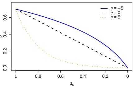
Figure 2: Examples of the rejection rate annealing function with different values of γ as defined in (12). Hereγ = −5,0, and5 respectively. A positive annealing rate would reduce the rejection rate quickly as the proportion of non-zeros weight values, ds, decreases, whereas a negative annealing rate would maintain it at a relatively high level.
To achieve the balance between exploration and exploitation, we construct an annealing function for the rejection rate that decreases monotonically as the level of sparsity decreases. Letβ0 ∈[0,1]
be the maximum rejection rate at initialization and let γ be the annealing rate. The annealing functionφfor the rejection rate at stages+ 1is given by
βs+1=φ(ds;β0, γ)
=
(
β0[exp (−γds)−dse−γ] γ ≥0;
β0log(1
−γ(1−ds))
log(1−γ) , γ <0,
(12)
whereds= |
ˆ Ωs|
p is the level of weight vector sparsity at the end of stages. The greater the valueγ is, the faster the rejection rate is annealed to zero as the number of stable features decreases.
A positive, zero and negative value of γ corresponds to exponential decay, linear decay and logarithmic decay of the rejection rate, respectively. Figure 2 presents examples of the rejection rate anneal function withγ =−5,0, and5respectively.
By using adaptive gravity (11) with annealed rejection rate (12), the amount of shrinkage is adjusted to the current level of sparsity of the weight vector quantified by the size of the stable set |Ωˆs|or theL0 norm of the purgedw˜. Instead of tuning a fixed gravity parameter as in (Langford
et al., 2009), for our proposed algorithm, we tune the annealing rateγ and the maximum rejection rateβ0. Hereγ balances the trade-off between exploration and exploitation andβ0 determines the
Algorithm 4Ψ(D): Stabilized truncated stochastic gradient descent for sparse learning.
Input:the training dataD.
Parameters: β0,γ,π0,K,nK,M,η.
Initialization: For eachm ∈ {1, . . . , M}, initializew˜(0m) =0p,k˜ =0pandD(m)is a random permutation ofD;Ωˆ0={1, . . . , p}.
Fors= 1,2, . . ., Setwˆ(0m) = ˜ws(m−1)
repeat
Obtaing0,s(βs)as in (11).
for allm∈ {1, . . . , M}parallel do forτ = 1tonK do
ˆ
w(τm) =B2
ˆ
w(τm−)1, g0,s(βs),Ωˆs−1,D(m)
.
end for end for
ComputeΠˆsas in (8) and update the set of stable featuresΩˆs=
n
j : ˆΠs,j≥π0 o
.
˜
ws(m)= ˆwn(mK)IΩˆs,m= 1, . . . , M.
βs+1=φ(ds;β0, γ)whereds= |
ˆ Ωs|
p .
Aggregation:w= M1 M
P
m=1
˜
w(sm).
untilwconverges.
Return: w.
permit fast reduction of the active set. The complete algorithm of the stabilized truncated stochastic gradient descent algorithm is summarized in Algorithm 4. .
4. Properties of the Stabilized Truncated Stochastic Gradient Descent Algorithm
The learning goal of sparse online learning is to achieve a low regret as defined in (3). In this section, we analyze the online regret bound of the proposed stabilized truncated SGD algorithm in Algorithm 4 with convex loss. For simplicity, the effect of adaptive gravity with annealed rejection rate is not considered here. To achieve viable result, we make the following assumptions.
Assumption 1 The absolute values of the weight vectorware bounded above, that is,|wj| ≤ C
for someC∈[0,∞),j= 1, . . . , p.
Assumption 2 The loss functionL(w, z)is convex inw, and there exist non-negative constantsA
andBsuch that, for allw∈Rpandz∈
Rp+1,||∇wL(w, z)||2 ≤AL(w, z) +B.
For linear prediction problems, the class of loss function that satisfies Assumption 2 includes common loss functions used in machine learning problems, such as theL2loss, the hinge loss and
the logistic loss, with the condition thatsupx||x|| ≤Cxfor some constantCx>0.
1. W is the parameter space for weight vectorswthat is subject to a sparsity constraint
||w||0 =d∗.
For the optimal weight vector w∗, we denote Ω∗ = {j : |wj∗| > 0} andd∗ = |Ω∗|. We further assume thatd∗ is sufficiently small and the gravity parameterg associated withw∗
is reasonably large so that, forτ = 1,2, . . ., the average number of active selected features from each truncated bursts,qg, given a gravityg, is greater than or equal tod∗.
2. Assume featuresx1, . . . ,xphas various sparsity distribution thatPr(|xi,j|>0) =λj, where
λj ∈[0,1], fori= 1, . . . , n, andwj∗= 0ifλj = 0, forj = 1, . . . , p.
Assumption 3 posits that w’s parameter space of interest is substantially sparse, which is the main focus of sparse learning and of this paper. The theoretical analysis in the following concerns for an fixed optimal weight vectorw∗, if exists, under such a constraint. Nevertheless, this condition does not confine the applicable scenarios of the proposed method to a fixed subclass of problems. It suggests a balance between the model sparsity and the value of the gravity parameter that is implicitly embedded within the parameter tuning process.
Assumption 4 LetΩ = {1, . . . , p} andN = Ω\Ω∗. Let ΩˆG = S
g∈GΩˆg∈G. Assume that the classifierfwis not worse than random guessing. That is,
E(|Ω∗TΩˆG|) E(|NTΩˆG|)
≥ |Ω ∗|
|N|.
Lemma 1 (Error Control in Stability Selection (Meinshausen and B ¨uhlmann, 2010)) LetV be the set of falsely selected variables. Given that the distribution of
n
Ij ∈Sˆg( ˆw;XK, j ∈1, . . . , po
is exchangeable for allg ∈ G and if Assumption 4 holds, the expected cardinality of |V|is then bounded forπ0 ∈ 12,1
by
E(|V|)≤ 1
2π0−1
(qg)2
p . (13)
Lemma 2 Assume all assumptions above holds. Let wˆ be a non-stabilized dense weight vector, i.e., an output weight vector from Algorithm 3. Let w˜ be the stabilized weight vector derived from wˆ, which is purged by the stability selection (10) with a set of stable features Ωˆ. Let qg
be the average number of nonzero entries inwˆ’s of the previous truncated bursts, i.e.,the number of
selected features fromnktruncated bursts, with gravityg. Then, there exists anε∈
0,π0C(p−|Ωˆ|)
|Ωˆ|
withSˆε ={j :E(|wˆj|) > ε}such that the bound on the expected difference between the distance
from the non-stabilized weight vector tow∗ and the distance from the stabilized weight vector to
w∗is given by
E ||wˆ −w∗||2− ||w˜ −w∗||2≥ ε2(|Sˆε| − |Ωˆ|) + 2π0C2
1− q
g
2π0p−p
qg−d∗
. (14)
When the purging threshold is sufficiently high such thatπ0∈
1 2 +
(qg)2 2p(qg−d∗),1
,
Proof: See Appendix A.
Lemma 2 quantifies the gain of using stabilization when w∗ is highly sparse, where stability selection efficiently shrinks high variable estimates to zero. When the purging threshold π0 is
sufficiently high such thatπ0 ∈
1 2 +
(qg)2 2p(qg−d∗),1
, the lower bound achieved by (14) is guaranteed to be positive. Furthermore, this result also indicates that the expected difference between distances from the non-stabilized and stabilized weight vector to the sparsew∗ depends on the differences between the sizes of the temporary nonzero set of features before purging,|Sˆε|, and the size of the stable features after purging. In expectation, the stabilized weight vector is closer to the target sparse weight vector as the operation of purging efficiently reduces the size of stable features. This suggests a much faster convergence with stabilization. Lemma 2 also provides an insight on the benefit from using adaptive gravity with annealed rejection rate. At the beginning of the algorithm, the gap between the size of |Sˆε| and the size of the set of stable features|ˆΩ|is large when aiming for extensive exploration of different sparse combination of features. Hence, the improvement brought by stabilization is more substantial during the early state of learning period. As the algorithm proceeds and the set of stable features becomes smaller and stabler, it dwindles the leeway that allows the aforementioned two sets to be different. Consequently, the proposed algorithm is gradually tuned toward the standard stochastic gradient descent algorithm to facilitate better convergence at the later period of the learning process.
Lemma 3 Letw0be the weight vector at initialization. After the first burst, letw¯1be the truncated weight vector using universal gravity g0K as in Algorithm 1 and letwˆ1 be the truncated weight vector with informative truncation as in Algorithm 2. Then, under Assumption 3,
E ||w¯1−w∗||2− ||wˆ1−w∗||2
≥2g0
K
X
t=1
kζtw∗k1 ≥0, (15)
whereζt,j =I(|xt,j|= 0)forj= 1, . . . , pandζt= (ζt,1, . . . , ζt,p)T.
Proof: See Appendix B.
In Lemma 3, we compare the distances towards w∗ from 1)the weight vector with uniform gravity and 2)the weight vector with informative truncation that depends on the number of zero entries occurred in a burst. Such a gap suggests the effectiveness of informative truncation on sparse data in which feature sparsity is highly heterogeneous. In the scenarios where very few nonzero entries appear in a burst, the informative truncation imposes gravity that is proportional to the information presented in a burst. It is a fairer treatment than uniform truncation and leads to a large improvement in expectation. When features are all considerably dense in a burst, the informative truncation is equivalent to the uniform truncation.
In short, Lemma 2 demonstrates the improvement in expected squared error due to stabilization on the weight vector. Lemma 3, on the other hand, quantifies the improvements in reduce truncation bias when implementing informative truncation on sparse features with heterogeneous sparsity levels.
Theorem 1 Assume all assumptions above holds. Consider the updating rules for the weight vector in Algorithm 3. On an arbitrary path, withw0 = 0andη >0, let{wt}Tt=1be the resulted weight
vector and
n g
t
oT
t=1 be the gravity values applied to the weight vectors generated by Algorithm 4,
along with the base gravity parameters
n g
0,t
oT
t=1. Set the purging thresholdπ0 to be sufficiently large such thatπ0 ∈
1 2 +
(qg)2 2p(qg−d∗),1
. There exists a sequence ofεt ∈
0,π0C(p−|Ωˆt|)
|Ωˆt|
at each
stability selection with the set of stable featuresΩˆtsuch that the expectation of the regret defined in (3)is bounded above by
E
T
X
t=1 h
L(wt, zt) +Kgt||wt||1 i − T X t=1 h
L(w∗, zt) +Kgt||w∗||1 i
!
≤ ηA
2−ηA E
" T X
t=1
L(w∗, zt) +Kg0,t(||w∗||1− ||wt||1) #!
+ 1
2−ηA
ηT B+ 1
η||w
∗||2
− 1
2η−η2A
T
X
t=1 ε2tI
t KnK
∈Z
(|Sˆεt,t| − |Ωˆt|), (16)
whereSˆε,t={j:E(|wˆt,j|)> εt}andwˆtis the weight vector at timetbefore stabilization.
Proof: See Appendix C.
In the result of Theorem 1, the first two parts of the right-hand-side of the expected regret bound (16) is similar to the bound obtained in (Langford et al., 2009). It implies the trade-off between attained sparsity in the resulted weight vector and the regret performance. When the applied gravity is small under the joint effect of the base gravityg0 and the size of each burst K, the sparsity is
less but the expected regret bound is lower. On the other hand, when the applied gravity is large, the resulted weight vector is more sparse but at the risk of higher regret. Based on Lemma 2, the proposed algorithm is guaranteed to achieve lower regret bound in expectation when the target sparse weight vector is highly sparse. As quantified in the third term of the right-hand-side of (16), the improvement comes from the reduction of the active set at each purging. By its virtue, noisy features are removed from the set of stable features and thus are absent in later SGD updates and truncations.
Theorem 1 is stated with a constant learning rateη. It is possible to obtain a lower regret bound in expectation with adaptive learning rateηtdecaying witht, such asηt= √1t, which is commonly used in the literature of online learning and stochastic optimization. However, the discussion of using an varying learning rate is not a main focus of this paper and adds extra complexity of the analysis. Without knowingT in advance, this may lead to a no-regret bound as suggested in (Langford et al., 2009). Instead, in Corollary 1, we show that the convergence rate of the proposed algorithm isO(√T)withη= √1
Corollary 1 Assume that all conditions of Theorem 1 are satisfied. Let the learning rateηbe √1 T.
The upper bound of the expected regret is
E
T
X
t=1 h
L(wt, zt) +gt||wt||1 i − T X t=1 h
L(w∗, zt) +gt||w∗||1 i
!
≤O(√T),
wheregt=Kg0,t.
Proof By plugging inη = √1
T to the result from Theorem 1, we get
E
T
X
t=1 h
L(wt, zt) +gt||wt||1 i − T X t=1 h
L(w∗, zt) +gt||w∗||1 i
!
≤ A
2√T−A E
" T X
t=1
L(w∗, zt) +gt(||w∗||1− ||wt||1 #!
+ T
2√T−A
ηT B+1
η||w
∗||2
− T
2√T −A
T
X
t=1
ε2tI( t
KnK
∈Z)(|Sˆε,t| − |Ωˆt|).
The result is then straightforward.
Assume that the input features have d nonzero entries on average. With linear prediction model fw(x) = wTx, the computational complexity at each iteration is O(d). Leveraging the sparse structure, the informative truncation only requires an additionalO(Kd)space for recording the counters. The purging process of stability selection consumes O(δ), δ = KnKM d, space for storing the generated intermediate weight vectors and O(δlog(δ))computational complexity. Both storage and computational cost decrease when the set of stable features diminishes as the algorithm proceeds. Since the parametersK, nK, and M is normally set to be small values, the complexity mostly depends onO(dlog(d)). In summary, the proposed algorithm scales with the number of nonzero entries instead of the total dimensions, making it appealing to high-dimensional applications.
5. Practical Remarks
When implementing Algorithm 4 in practice, the performance can be further improved in terms of both accuracy and computational efficiency by employing a couple of practical techniques. It includes applying informative purgingand attenuating the truncation frequency to achieve more accurate sparse learning and steadier convergence.
The first improvement can be implemented by better addressing the issue of scarcity of incoming samples. For computing selection probabilities, instead of using only information from the current stage, we can inherit information from previous stages for features that are too scarce to accumulate enough updates during one stage. Specifically, we introduce anaccumulated counterκsat stages as the total number of times that a feature is updated within a burst during this stage:
κj,s= M X m=1 nK X τ=1 ˜
which is essentially the denominator of the selection probability in (8). Similarly, we define an accumulated truncation indicatorbsat stagesas the total number of times that a feature is truncated to zero given valid update(s):
bj,s= M
X
m=1 X
τ:˜k(j,τm)>0
I(|wˆj,τ(m)|>0), j= 1, . . . , p.
A feature is then evaluated in the stability selectiononlyif there are enough updates from the present stage and from any unused information carried over from previous stages. Given a threshold
δK ≥ 0, letκ˜j,s , κ˜j,s−1I(˜κj,s−1 < δK) +κj,sandb˜j,s , b˜j,s−1I(˜κj,s−1 < δK) +bj,s. The selection probability is modified as
ˆ Πj,s=
( ˜
bj,s
˜
κs , forjs.t.κ˜s> δK;
1, otherwise, forj= 1, . . . , p. (17)
This strategy extends the key idea in Section 3.1 that, with sparse data, each decision need to be based on sufficient evidence. Using the “carried-over” information allows the algorithm to utilize information available in a sequence of SGD updates while attuned to the needs of features with different levels of sparsity. In practice, this modification facilitates faster convergence especially for ultra-sparse data.
The second practical strategy is that the size of each burst,K, can be adaptively adjusted in a similar fashion as the rejection rateβ in (12). At the end of each stage, the burst sizeKsis updated as
Ks=
l K0log
1
αds−1
m ,
where K0 > 0 is the initial burst size and, as in (12), ds = |
ˆ Ωs|
p . The tuning parameter α > 0 adjusts the annealing rate of the truncation frequency. Although the result in Theorem 1 is based on a fixedK, it can be easily shown that the same upper bound can also be attained with an increasing
Ks. By increasingK in the later stage of the algorithm, when the majority of irrelevant features have been removed from the stable set, the chance of erroneous truncation is reduced. Such scheme further steers the algorithm from the mode of exploring potential sparse combination of features in the early stage toward the fine tuning of the weight vector by exploiting information from more samples in a sequence. It also facilitates faster convergence as the size of the stable set approaches to a sufficiently small number, as the algorithm converges to the standard stochastic gradient descent approximately.
6. Results
In this section, we present experimental results evaluating the performance of the proposed sta-bilized truncated SGD algorithm in high-dimensional classification problems with sparsity reg-ularization. In this paper, we focus on linear prediction model for binary classification where
fw(x) =wTxandyˆ=sign(fw(x))with the observed class labely ∈ {−1,1}. We consider two commonly used convex loss functions in machine learning tasks that both satisfy Assumption 1:
• Logistic loss:l(f, y) = log (1 + exp(−f y)).
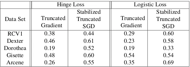
Using five data sets from different domains, the performance of our algorithm and other algo-rithms for comparison are evaluated on classification performance and feature selection stability and sparsity. We first define measure of feature stability in Section 6.1.
6.1 Feature Selection Stability
The goal of sparse learning is to select a subset of truly informative features with stabilized estima-tion variance as well as increased classificaestima-tion accuracy and model interpretability. Subgradient-based online learning methods depend heavily by the random ordering of samples on which they are fed to the algorithm. Such dependence leads to much deteriorated performance when it comes to high-dimensional sparse inputs. For a particular feature, the positions of its nonzero occurrences in a random ordering of samples greatly affect its learning outcome, in terms of learnt weight and membership in the set of selected features. Therefore, in addition to attaining a low generalization error, a desirable sparse online learning method should also produce an informative feature subset that is stable and robust to random permutations of input data. To evaluate feature selection stability of subgradient-based sparse learning methods, we define in the following a numerical measure of similarity between selected feature subsets resulted from different random permutations of data. Given an output weight vectorwfrom a subgradient-based algorithm with input dataD, similarly as in (6), we denote the selected feature subset as
S(w;D) ={j:|wj|>0,w= Ψ(D}.
Given two random permutations of the training data D,D(1) andD(2), the similarity between
the two sets of selected feature subsetsS1 = S(w1;D(1))andS2 = S(w2;D(2))is measured by
the Cohen’s kappa coefficient introduced by Cohen (1960),
κ(S1,S2) = qo−qe 1−qe
,
whereqois therelative observed agreementbetweenS1andS2:
qo=
p11+p22 p ,
andqeis thehypothetical probability of change agreement:S1andS2
qe =
(p11+p12)(p11+p21)
p2 +
(p12+p22)(p21+p22) p2 ,
withp11=|S1∩ S2|,p12=|S1∩ S2C|,p21=|S1C ∩ S2|,p22=|S1C ∩ S2C|, andp=p11+p12+ p21+p22is the size of variable pool.
Note thatκ(S1,S2)∈[−1,1], whereκ(S1,S2) = 1ifS1andS2completely overlap with each other and κ(S1,S2) = −1whenS1 andS2 are in complete disagreement withS1 ∩ S2 = ∅and SC
1 ∩ S2C =∅.
Based on Cohen’s kappa coefficient, we define the measure of feature selection stability of S(w;·)returned by a procedureΨusing randomly ordered dataD(1)andD(2)as
s(Ψ) =ED(1),D(2) h
κ(S(w1;D(1)),S(w2;D(2))
which is motivated by (Sun et al., 2013).
In practice, we use the empirical averagesˆ(Ψ)overBrandom permutations of the training data to measure the stability of the a subgradient-based online learning algorithmΨ(·):
ˆ
s(Ψ) = 1
B(B−1) D
X
i=1 X
j6=i
h
κ(Swi;D(i)),S(wj;D(j))i. (18)
6.2 Experiment Setup
We evaluate the performance of our algorithm on several real-world classification data sets with up to100,000features. These data sets have different levels of sparsity with various sample sizes. The information of experiment data sets are summarized in Table 1. The first four data sets were constructed for NIPS 2003 Feature Selection Challenge4(see Guyon et al., 2004, for details), which were preprocessed with added “probes” as random features distributed similarly to the real features. Thus, a good performance does not only lie in low generalization error rates, but also in sparse weight vectors that identify the truly important features. Reuters CV1 (RCV1) is a popular text classification data set with a bag-of-words representation. We use the binary version from the LIBSVM data set collection5introduced by Cai and He (2012). We create the training and validation set using a 70-30 random splits. All datasets are normalized such that each feature has variance 1.
Data Set Domain Dimensions Data Density (Sparsity)
Training Size
Validation Size
RCV1 Text Mining 47,236 0.16% 14,169 6,073
Dexter Text Mining 20,000 0.48% 300 300
Dorothea Drug Discovery 100,000 0.91% 800 350
Gisette Digits Recognition 5,000 13.00% 6,000 1,000
Arcene Mass-Spectrometry 10,000 50.00% 100 100
Table 1: Datasets used in the numerical experiments. Sparsity is defined as the average feature sparsity levels, which is the column-wise average percentage of nonzero entries, in the training data.
We compare the proposed algorithm with the standard stochastic gradient descent algorithm in (Bottou, 1998) and another three other sparsity-inducing stochastic methods, including the truncated gradient algorithm in (Langford et al., 2009), the Regularized Dual Averaging (RDA) algorithm in (Xiao, 2009), and the forward backward splitting (FOBOS) algorithm in (Duchi and Singer, 2009). The RDA algorithm updates the weight vector at each step based on a running averageg¯tof all subgradients{gτ =L0(wτ, zτ)∈∂wτL(wτ, zτ), τ = 1, . . . , t}in previous iterations as
¯
gt=
t−1
t gt−1+
1
tgt.
4. The data source can be found onhttps://archive.ics.uci.edu/ml/index.html.
5. The data source can be found on https://www.csie.ntu.edu.tw/˜cjlin/libsvmtools/
Given the average subgradient , the next weight vector is computed by solving the minimization problem
wt+1=argmin
w
(
1
t
t
X
τ
hL0(wt, zt),wi+ Ψ(w) +
βt
t h(w) )
, (19)
where Ψ(w) is the regularizer, h(w) is an auxiliary strongly convex function, and{βt}t≥1 is a
nonnegative and nondecreasing input sequence, which determines the convergence properties of the algorithm.
In the context ofL1regularization, the RDA algorithm is derived by settingΨ(w) =λ||w||1, βt=γ
√
t, and replacingh(w)with a parametrized version:
hρ= 1 2||w||
2
2+ρ||w||1,
where ρ ≥ 0 is a sparsity-enhancing parameter. Hence, the minimization problem in (19) has a explicit solution as, forj= 1, . . . , p,
wt(j+1) =
(
0, if|g¯(tj)| ≤λRDAt ;
− √
t γ
¯
g(tj)−λRDAt sgn(¯g(tj)), otherwise,
which is equivalent to
wt+1 =T(¯gt, λRDAt ),
whereλRDAt =λ+γρ/√t.
The FOBOS algorithm alternates between two phases. On each iteration, it first perform an unconstrained gradient descent step as in the standard SGD algorithm, whose output is denoted aswt+1
2. Then it cast and solve an instantaneous optimization problems that trades off between
minimization of a regularization term and a close proximity to the result of the first phase:
wt+1=argmin
w
1
2||w−wt+12|| 2+η
t+12Ψ(w)
, (20)
where the regularization function is scaled by an interim step sizeηt+1
2.
WithL1regularization whereΨ(w) =λ||w||1, the second-phase update can be computed as
wt+1=T(wt+1
2, ηt+
1
2λ).
To evaluate the stability of resulted weight vectors, we randomly permute the indices of the training samples forB = 50 times to produce stochastic samples that are fed to the algorithms. Such randomization helps identify the instability in learning results in terms of both error rate and the selected features.
λfrom the set of values{5×10−5,1×10−4,5×10−4,1×10−3,0.01,0.05,0.1,0.5,1,5,10}for both RDA and FOBOS. As instructed by Duchi and Singer (2009),ηtis set to be √1tin FOBOS. For the proposed stabilized truncated SGD algorithm, the size of each burst (the truncation frequency) is fixed at K = 5 and nK = 5 for all data sets. In the proposed algorithm, we initiate the rejection rate atβ0 = 0.7with annealing rate chosen from{−7,−5,−3,−1,0,1,3}. The stability
selection thresholdπ0is tuned within the range[0.5,0.6, . . . ,0.9]. For multi-thread implementation
in Algorithm 4,M = 16is used running in parallel on a high-performance computing cluster.
6.3 Results
6.3.1 CLASSIFICATIONPERFORMANCE
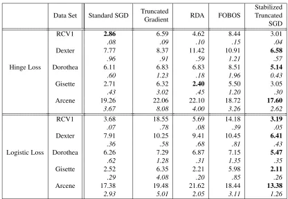
As shown in Table 2, the proposed algorithm shows improvement over the truncated gradient algorithm over all data sets and has better performances than RDA and FOBOS in most of the experiments. As data density increases, the truncated gradient algorithm performs better with hinge loss than with logistic loss. With hinge loss, the algorithm updates the weight vector only for samples within a small margin from the boundary. With logistic loss, the algorithm updates with continuous increments for all incoming samples and favors dense features in sparse learning. With highly sparse samples sequentially feed to the algorithm, the truncation in every K iterations is conducted with insufficient information about the true gradient due to the lack of nonzero entries in sparse features. Truncation with logistic loss leads to over selection of dense features and overfitting. The other two sparsity-inducing methods for comparison, RDA and FOBOS, also have large fluctuations across data sets with different levels of sparsity over these two loss functions, especially when data is highly sparse. In comparison, the performance of the proposed algorithm is consistent for various dimensions and sparsity levels. Our algorithm is also shown to be robust to different choices of loss function. The comparatively lower test errors, especially for highly sparse data, mainly owes to the proposed algorithm’s fairer treatments of features with heterogeneous sparsity.
From Table 2 we also observe substantially lower variances in test errors under random per-mutations of samples. The proposed algorithm has the lowest standard deviations of test errors across all data sets and under both loss functions. Such an improvement over truncated gradient algorithm and other comparing methods comes from both informative truncation with adaptive gravity and stability selection. Based on these selection probabilities we carry out feature purging. Our selection probability is computed based on multiple bursts whose truncation is guided by fair amounts of shrinkage. Hence, the removal decisions of features from the set of stable variables are grounded in reliable information on feature importance, which is more likely to be shared across different permutations of the data. The accumulations of sufficient information for all features help the proposed algorithm to be robust to random fluctuations in online setting.
6.3.2 FEATURESELECTION ANDSPARSITY
Data Set Standard SGD Truncated
Gradient RDA FOBOS
Stabilized Truncated SGD
RCV1 2.86 6.59 4.62 8.44 3.01
.08 .09 .10 .15 .04
Dexter 7.77 8.37 11.42 10.91 6.58
.96 .91 .59 1.21 .57
Hinge Loss Dorothea 6.11 6.83 6.83 8.51 5.14
.60 1.23 .18 1.96 0.43
Gisette 2.71 6.32 2.40 5.50 3.05
.43 3.02 .45 1.20 .30
Arcene 19.26 22.06 22.10 18.72 17.60
3.67 8.08 4.00 3.26 2.62
RCV1 3.68 18.55 5.69 14.18 3.19
.07 .78 .08 .39 .05
Dexter 7.91 10.25 9.41 10.45 6.41
.36 .58 .68 .81 .43
Logistic Loss Dorothea 6.26 7.29 6.87 7.15 5.47
.62 1.28 .31 1.35 .35
Gisette 2.52 6.35 2.21 5.98 2.11
.29 4.08 .20 .85 .26
Arcene 17.38 19.48 21.62 18.44 13.38
2.93 5.01 2.05 3.11 1.26
Table 2: Mean test errors (%) and the corresponding standard deviations with hinge loss and logistic loss over 50 random ordering of the training samples.
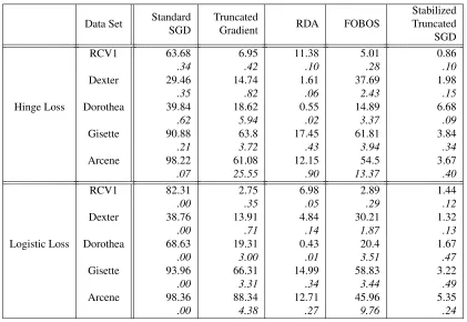
function and when the sparsity level of the input data is low, such as the case of the Arcene data set. These results also indicate that the truncate gradient algorithm fails to extract significant features and to obtain sparse solutions, which motivates the development of techniques discussed in this paper. On the other hand, the variances in the percentage of nonzero features of the proposed algorithm are reduced by approximately a magnitude of 10. The contribution of stabilization is demonstrated again in terms of feature selection. Although RDA achieves very low sparsity in Dorothea, such a behavior is not observed in other data sets. It is shown to result in particularly denser weight vector with highly sparse data, such as RCV1, indicating its weakness in identifying truly informative features when information is scarce. FOBOS demonstrates overall poorer performance in terms of inducing sparse weight vector as compared to RDA and the proposed algorithm. Similar to its performance in terms of test error, the proposed algorithm delivers highly stable results in feature selection regardless of the choice of loss function and of random permutations of the data. We also achieve sufficient sparse result owing to stability selection which prevent noisy features from adding back to the stable set of variables in the online setting. On the other hand, the high sparsity in weight vector does not overshadow the generalizability performance as the informative truncation with unbiased shrinkage underlies a better estimation of the selection probability for the construction of the set of stable variables.
Data Set Standard SGD
Truncated
Gradient RDA FOBOS
Stabilized Truncated SGD
RCV1 63.68 6.95 11.38 5.01 0.86
.34 .42 .10 .28 .10
Dexter 29.46 14.74 1.61 37.69 1.98
.35 .82 .06 2.43 .15
Hinge Loss Dorothea 39.84 18.62 0.55 14.89 6.68
.62 5.94 .02 3.37 .09
Gisette 90.88 63.8 17.45 61.81 3.84
.21 3.72 .43 3.94 .34
Arcene 98.22 61.08 12.15 54.5 3.67
.07 25.55 .90 13.37 .40
RCV1 82.31 2.75 6.98 2.89 1.44
.00 .35 .05 .29 .12
Dexter 38.76 13.91 4.84 30.21 1.32
.00 .71 .14 1.87 .13
Logistic Loss Dorothea 68.63 19.31 0.43 20.4 1.67
.00 3.00 .01 3.51 .47
Gisette 93.96 66.31 14.99 58.83 3.22
.00 3.31 .34 3.44 .49
Arcene 98.36 88.34 12.71 45.96 5.35
.00 4.38 .27 9.76 .24
Table 3: The average percentages (%) of nonzero features selected in the resulted weight vector and the corresponding standard deviations with hinge loss and logistic loss over 50 random permutations of the training samples.
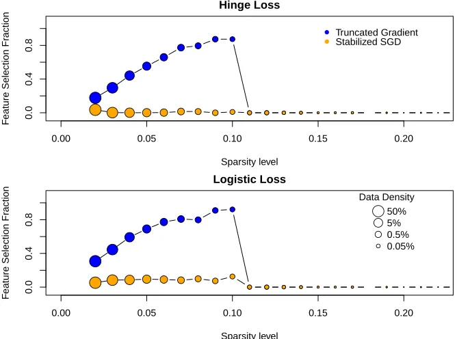
of selected features at different data density levels. It is shown that truncated gradient algorithm is more likely to select dense features over sparse ones with both loss functions. The majority of the sparse features are truncated to zero regardless of their importance. Moreover, the fraction of selected feature exhibits a linear relationship with the level of feature density in truncated gradi-ent algorithm. This pattern suggests that the amount of shrinkage applied to features should be approximately proportional to their data density, on the probability of having informative updates. This provides an independent justification of the informative truncation introduced in Section 3.1. In contrast, features selected by the proposed algorithm have approximately uniform distribution of sparsity levels. This improvement over the truncated gradient algorithm mostly owes to the use of informative truncation. With the crucial treatment on the heterogeneity in feature sparsity, the proposed algorithm is effective in keeping rare but important features from premature truncations.
●●
● ●
● ●
● ● ●
● ● ● ● ● ● ● ● ● ● ● ●
0.00 0.05 0.10 0.15 0.20
0.0
0.4
0.8
Hinge Loss
Sparsity level
F
eature Selection Fr
action
●● ● ● ● ● ● ● ● ● ● ● ● ● ● ● ● ● ● ● ●
●
● Truncated GradientStabilized SGD
●●
● ●
● ● ●
● ●
● ● ● ● ● ● ● ● ● ● ● ●
0.00 0.05 0.10 0.15 0.20
0.0
0.4
0.8
Logistic Loss
Sparsity level
F
eature Selection Fr
action
●● ● ● ● ● ● ● ●
● ● ● ● ● ● ● ● ● ● ● ●
Data Density
●
●
●
●
50% 5% 0.5% 0.05%
Figure 3: The fraction of features selection at different sparsity levels by the truncated gradient algorithm and the proposed algorithm respectively with the Dorothea data set as an example. The selected features are extracted as the features with nonzero entries in the resulted weight vector from the algorithms with a single fixed ordering of the training data. Thex-axis represents the sparsity level, which is the proportion of nonzero entries in a feature in the training sample. They-axis indicates the fraction of selected features among features with a discretized sparsity level. The size of each point scales with the proportion of features that fall in level of sparsity. It can be seen that the truncated gradient algorithm over-selects denser features. The proposed algorithm does not have a pre-exposed preference towards any density level.
sufficient accumulations of information in selection probabilities before applying stability selection. These measures suggest that the proposed algorithm is particularly favorable for high-dimensional sparse data.
7. Conclusion