Reward Maximization Under Uncertainty: Leveraging Side-Observations on Networks

Reward Maximization Under Uncertainty: Leveraging

Side-Observations on Networks

Swapna Buccapatnam [email protected]

AT&T Labs Research, Middletown, NJ 07748, USA

Fang Liu [email protected]

Atilla Eryilmaz [email protected]

Department of Electrical and Computer Engineering The Ohio State University

Columbus, OH 43210, USA

Ness B. Shroff [email protected]

Department of Electrical and Computer Engineering and Computer Science Engineering The Ohio State University

Columbus, OH 43210, USA

Editor:Shie Mannor

Abstract

We study the stochastic multi-armed bandit (MAB) problem in the presence of side-observations across actions that occur as a result of an underlying network structure. In our model, a bipartite graph captures the relationship between actions and a common set of unknowns such that choosing an action reveals observations for the unknowns that it is connected to. This models a common scenario in online social networks where users respond to their friends’ activity, thus providing side information about each other’s preferences. Our contributions are as follows: 1) We derive an asymptotic lower bound (with respect to time) as a function of the bi-partite network structure on the regret of anyuniformly good policythat achieves the maximum longterm average reward. 2) We propose two policies -a r-andomized policy; -and -a policy b-ased on the well-known upper confidence bound (UCB) policies - both of which explore each action at a rate that is a function of its network po-sition. We show, under mild assumptions, that these policies achieve the asymptotic lower bound on the regret up to a multiplicative factor, independent of the network structure. Finally, we use numerical examples on a real-world social network and a routing example network to demonstrate the benefits obtained by our policies over other existing policies. Keywords: Multi-armed Bandits, Side Observations, Bipartite Graph, Regret Bounds

1. Introduction

Multi-armed bandit (MAB) problems are well-known models of sequential decision-making under uncertainty (Lai and Robbins, 1985) and have lately been used to model new and ex-citing decision problems in content recommendation systems, online advertising platforms, and social networks, among others. In the classical MAB setting, at each time, a bandit policy must choose an action from a set of actions with unknown probability distributions. Choosing an action gives a random reward drawn from the distribution of the action. The regret of any policy is defined as the difference between the total reward obtained from the

c

action with the highest average reward and the given policy’s total reward. The goal is to find policies that minimize the expected regret over time.

In this work, we consider an important extension to the classical MAB problem, where choosing an action not only generates a reward from that action, but also reveals important information for a subset of the remaining actions. We model this relationship between different actions using a bipartite graph between the set of actions and a common set of unknowns (see Figure 2). The reward from each action is a known function of a subset of the unknowns (called its parents) and choosing an action reveals observations from each of its parents. Our main objective in this work is to leverage such a structure to improve scalability of bandit policies in terms of the action/decision space.

Such an information structure between actions becomes available in a variety of appli-cations. For example, consider the problem of routing in communication networks, where packets are to be sent over a set of links from source to destination (called a path or a route) in order to minimize the delay. Here, the total delay on each path is the sum of individual link delays, which are unknown. In addition, traveling along a path reveals observations for delays on each of constituent links. Hence, each path provides additional information for all other paths that share some of their links with it. In this example, actions correspond to a set of feasible paths and the set of unknowns corresponds to random delays on all the links in the network.

Another example occurs in advertising in online social networks through promotional offers. Suppose a user is offered a promotion/discounted price for a product in return for advertising it to his friends/neighbors in an online social network. The influence of the user is then measured by the friends that respond to his message through comments/likes, etc. Each user has an intrinsic unknown probability of responding to such messages on social media. Here, the set of actions correspond to the set of users (to whom promotions are given) and the set of unknowns are the users’ intrinsic responsiveness to such promotions.

In this work, we aim to characterize the asymptotic lower bound on the regret for a general stochastic multi-armed bandit problem in the presence of such an information structure and investigate policies that achieve this lower bound by taking the network structure into account. Our main contributions are as follows:

• We model the MAB problem in the presence of additional structure and derive an asymptotic (with respect to time) lower bound (as a function of the network structure) on the regret of any uniformly good policy which achieves the maximum long term average reward. This lower bound is presented in terms of the optimal value of a linear program (LP).

• Motivated by the LP lower bound, we propose and investigate the performance of a randomized policy, we callt-greedy-LP policy, as well as an upper confidence bound

based policy, we call UCB-LP policy. Both of these policies explore each action at a rate that is a function of its location in the network. We show under some mild assumptions that these policies are optimal in the sense that they achieve the asymp-totic lower bound on the regret up to a multiplicative constant that is independent of the network structure.

number of actions becomes large, significant benefits can be obtained from policies that explicitly take network structure into account. While t-greedy-LP policy explores actions

at a rate proportional to their network position, its exploration is oblivious to the average rewards of the sub-optimal actions. On the other hand, UCB-LP policy takes into account both the upper confidence bounds on the mean rewards as well as network position of different actions at each time.

2. Related Work

The seminal work of Lai and Robbins (1985) showed that the asymptotic lower bound on the regret of any uniformly good policy scales logarithmically with time with a multiplicative constant that is a function of the distributions of actions. Further, Lai and Robbins (1985) provide constructive policies called Upper Confidence Bound (UCB) policies based on the concept of optimism in the face of uncertainty that asymptotically achieve the lower bound. More recently, Auer et al. (2002) considered the case of bounded rewards and propose simpler sample-mean-based UCB policies and a decreasing-t-greedy policy that achieve

logarithmic regret uniformly over time, rather than only asymptotically as in the previous works.

The traditional multi-armed bandit policies incur a regret that is linear in the number of suboptimal arms. This makes them unsuitable in settings such as content recommendation, advertising, etc, where the action space is typically very large. To overcome this difficulty, richer models specifying additional information across reward distributions of different ac-tions have been studied, such as dependent bandits by Pandey et al. (2007), X-armed bandits by Bubeck et al. (2011), linear bandits by Rusmevichientong and Tsitsiklis (2010), contextual side information in bandit problems by Li et al. (2010), combinatorial bandits by Chen et al. (2013) etc..

More recently, Cohen et al. (2016), have studied the multi-armed bandit problem with a graph based feedback structure similar to Mannor and Shamir (2011), and Buccapatnam et al. (2014). However, they assume that the graph structure is never fully revealed. In contrast, in many cases such as the problem of routing in communication networks and the problem of influence maximization in social networks, the graph structure is revealed or learnt apriori and is known. When the graph structure is known, the authors in Buccap-atnam et al. (2014) propose algorithms for the stochastic setting whose regret performance is bounded by the domination number of the graph. In contrast, the algorithms proposed in Cohen et al. (2016) assume that the graph is unknown and achieve a regret that is upper bounded by the independence number of the graph. (Note that the independence number of a graph is larger than or equal to the domination number). Our current work proposes a general feedback structure of which Buccapatnam et al. (2014) and Cohen et al. (2016) can be viewed as a special case. Moreover, we present algorithms that benefit significantly from the knowledge of the graph feedback structure.

The setting of combinatorial bandits (CMAB) by Chen et al. (2013) is also closely related to our work. In CMAB, a subset of base actions with unknown distributions form super actions and in each round, choosing a super action reveals outcomes of its constituent actions. The reward obtained is a function of these outcomes. The number of super actions and their composition in terms of base actions is assumed to be arbitrary and the policies do not utilize the underlying network structure between base actions and super actions. In contrast, in our work, we derive a regret lower bound in terms of the underlying network structure and propose policies that achieve this bound. This results in markedly improved performance when the number of super actions is not substantially larger than the number of base actions.

3. Problem Formulation

In this section, we formally define the general bandit problem in the presence of side observa-tions across acobserva-tions. Let N ={1, . . . , N}denote the collection ofbase-arms with unknown distributions. Subsets of base-arms form actions, and are indexed by K ={1, . . . , K}. A decision maker must choose an action j ∈ K at each time t and observes the rewards of related base-arms. Let Xi(t) be the reward of base-arm i observed by the decision maker

(on choosing some action) at time t. We assume that {Xi(t), t ≥0} are independent and

identically distributed (i.i.d.) for each iand{Xi(t),∀i∈ N } are independent for each time

t. Let Vj ⊆ N be the subset of base-arms that are observed when playing action j. Then,

we define Si = {j : i ∈ Vj} as the support of base-arm i, i.e., the decision maker gets

observations for base-arm i on playing action j ∈ Si. When the decision maker chooses

actionj at timet, he or she observes one realization for each of the random variablesXi(t),

i∈Vj. The reward of the played actionjdepends on the outcomes of its related base-arms

subset, denoted by K_j ⊆ N, and some known function fj(·). Note that Kj ⊆ Vj because

there may be some base-arms that can be observed by actionjbut not counted as reward in general (see Figure 2 for a concrete example). Let the vectorX~j(t) = [Xi(t)]i∈Kj denote the collection of random variables associated with the reward of actionj. Then the reward from playing actionj at timetis given byfj(X~j(t)). We assume that the reward is bounded in

and the specific form of fj(·) and Kj are determined by the decision maker or the specific

problem. Letµj be the mean of reward on playing actionj.

Side-observation model : The actions K and base-arms N form nodes in a network

G, represented by a bipartite graph (K,N, E) and the collection {Kj}j∈K. The N ×K

adjacency matrix E = [eij] is defined byeij = 1 if i∈Vj and eij = 0 otherwise. If there is

an edge between actionj and base-arm i, i.e.,eij = 1, then we can observe a realization of

base-armiwhen choosing actionj. Intuitively, the bipartite graph determined by{Vj}j∈K describes the side-observation relationships while the collection{K_j}_j∈Kcaptures the reward structure. Without loss of generality, we assume that∪i∈KKi =N, which means that there

are no useless (dummy) unknown base-arms in the network.

User i

User j

User k

User m

X

(t)

X

(t)

X

(t)

Figure 1: At time t, suppose that the decision maker chooses user i to offer a promotion. He then receives a responseXi(t) from user i. Using the social interconnections,

he also observes responsesXj(t) and Xk(t) of i’s neighborsj andk.

Figure 1 illustrates the side-observation model for the example of targeting users in an online social network. Such side observations are made possible in settings of online social networks like Facebook by surveying or tracking a user’s neighbors’ reactions (likes, dislikes, no opinion, etc.) to the user’s activity. This is possible when the online social network has a survey or a like/dislike indicator that generates side observations. For example, when useriis offered a promotion, her neighbors may be queried as follows: “Useriwas recently offered a promotion. Would you also be interested in the offer?1”

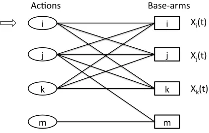
Figure 2 shows the bipartite graph generated from the example shown in Figure 1. The set of base-arms is the set of users since they act independently according to their own preferences in the promotion, which are unknown to the decision maker. The set of actions is also the set of users because the decision maker wants to target the users with the maximum expected reward. When actionj (userj) is chosen, the decision maker observes

Xi(t), Xj(t), Xk(t) and Xm(t) from user i,j,k and m since Vj ={i, j, k, m}. The reward

of playing action j depends on Kj and fj(·). Suppose fj(X~j(t)) = P_i∈KjXi(t). Then

Kj = {i, j, k, m} means that the reward is the sum of all positive feedbacks. It is also

i

j

k

m Base-arms Ac.ons

i

j

k

m

Xi(t)

Xj(t)

Xk(t)

Figure 2: Bipartite graph for the example of targeting users in online social network.

possible that the decision maker set Kj = {j}, which means that the reward of playing

actionj is only the observation from the userj.

The reward function can be quite general (but bounded) to accommodate different settings. Also, the bipartite graph can be more general than social networks in two key ways: 1) Connecting two users in two-hop neighborhood means that the reaction of the friend of my friend is also observable, which is true in Facebook. 2) Connecting two users, say i and j, with similar preference profiles means that the network actively recommends the promotion received by userito userj even though they are not friends. This has been widely applied in recommender systems such as Yelp.

Objective: An allocation strategy or policyφchooses the action to be played at each time. Formally, φ is a sequence of random variables {φ(t), t ≥ 0}, where φ(t) ∈ K is the action chosen by policyφat time t. LetT_jφ(t) be the total number of times action j is chosen up to timetby policyφ.For each action, rewards are only obtained when the action is chosen by the policy (side-observations do not contribute to the total reward). Then, the regret of policyφat time tfor a fixedµ= (µ1, . . . , µK) is defined by

Rφ_µ(t) =µ∗t−

K

X

j=1

µjE[Tjφ(t)] = K

X

j=1

∆jE[Tjφ(t)],

where ∆j , µ∗−µj and µ∗ ,max

j∈K µj. Henceforth, we drop the superscript φ unless it is required. The objective is to find policies that minimize the rate at which the regret grows as a function of time for every fixed network G. We focus our investigation on the class of uniformly good policies (Lai and Robbins, 1985) defined below:

Uniformly good policies: An allocation rule φis said to be uniformly good if for every fixed µ,the following condition is satisfied as t→ ∞:

Rµ(t) =o(tb), for everyb >0.

Definition 1 A hitting set D is a subset of K such that Si∩D 6= ∅, ∀i∈ N. Then the

hitting set number is γ(G) = infD⊆K{|D| : Si∩D 6= ∅, ∀i ∈ N }. For example, the set

{i, m} is a hitting set in Figure 2.

Definition 2 A cliqueC is a subset ofK such thatK_j ⊆Vi,∀i, j∈C. This means that for

every actioniinC, we can observe the reward of playing any action j inC. A clique cover

C of a network G is a partition of all its nodes into sets C ∈ C such that the sub-network formed by each C is a clique. Let χ¯(G) be the smallest number of cliques into which the nodes of the network G can be partitioned, also called the clique partition number.

Proposition 3 For any network G with bipartite graph(K,N, E)and{Kj}j∈K, if∪j∈KKj =

N, then γ(G)≤χ¯(G).

Proof LetC={C1, C2, ..., Cm}be a clique cover with cardinalitym, i.e.,|C|=mand each

Ck is a clique fork = 1, ..., m. Pick arbitrarily an element ak from Ck for each k. Define

H = {ak : k = 1, ..., m}. Now it remains to show that H is a hitting set, which implies

γ(G)≤χ¯(G). We prove this by contradiction.

Suppose H is not a hitting set, then ∃i ∈ N s.t. Si ∩ H = ∅. Since ∪j∈KKj = N,

∃j ∈ K s.t. i∈ Kj. C is a clique cover, then∃k(j)∈ {1,2, ..., m} such that j ∈Ck(j). By

the construction of H, there exists ak(j) ∈ H ∩Ck(j). By the definition of clique, we have K_j ⊆ Vak(j). Thus, we have ak(j) ∈ Si since i ∈ Kj. It follows that Si∩ H 6= ∅, which contradicts toSi∩ H=∅. Hence,H is a hitting set.

In the next section, we obtain an asymptotic lower bound on the regret of uniformly good policies for the setting of MABs with side-observations. This lower bound is expressed as the optimal value of a linear program (LP), where the constraints of the LP capture the connectivity of each action in the network.

4. Regret Lower Bound in the Presence of Side Observations

In order to derive a lower bound on the regret, we need some mild regularity assump-tions (Assumpassump-tions 1, 2, and 3) on the distribuassump-tions Fi (associated with base-arm i) that

are similar to the ones in Lai and Robbins (1985). Let the probability distribution Fi

have a univariate density function g(x;θi) with unknown parameters θi, for each i ∈ N.

Let D(θ||σ) denote the Kullback Leibler (KL) distance between distributions with density functions g(x;θ) and g(x;σ) and with meansu(θ) and u(σ) respectively.

Assumption 1 (Finiteness) We assume thatg(·;·)is such that0< D(θ||σ)<∞whenever u(σ)> u(θ).

Assumption 2 (Continuity) For any > 0 and θ, σ such that u(σ) > u(θ), there exists η >0 for which |D(θ||σ)−D(θ||ρ)|< whenever u(σ)< u(ρ)< u(σ) +η.

Assumption 3 (Denseness) For eachi∈ N, θi ∈Θwhere the setΘsatisfies: for allθ∈Θ

Let ~θbe the vector [θ1, . . . , θN]. Define Θi ={~θ:∃k∈Si such thatµk(~θ)< µ∗(~θ)}.So,

not all actions that support base-armiare optimal. Suppose~θ∈Θi.For base armi,define

the set

B_i(θi) ={θ0i :∃k∈Si such that µk(~θi0)> µ∗(~θ)},

where ~θ0_i = [θ1, . . . , θi0, . . . θN]. ~θi0 differs from ~θ only in the ith parameter. In this set

B_i(θi), base-arm i contributes towards a unique optimal action. Define constant Ji(θi) =

inf{D(θi||θ0i) :θ0i∈ Bi(θi)}.This is well-defined whenBi(θi)6=∅.

The following proposition is obtained using Theorem 2 in Lai and Robbins (1985). It provides an asymptotic lower bound on the regret of any uniformly good policy under the model described in Section 3:

Proposition 4 Suppose Assumptions 1, 2, and 3 hold. Let U ={j:µj < µ∗} be the set of

suboptimal actions. Also, let ∆j =µ∗−µj. Then, under any uniformly good policy φ, the

expected regret is asymptotically bounded below as follows:

lim inf

t→∞

Rµ(t)

log(t) ≥cµ, (1)

where cµ is the optimal value of the following linear program (LP) P1:

P1 : minX

j∈U ∆jwj,

subject to: X

j∈Si

wj ≥

1

Ji(θi)

, ∀i∈ N,

wj ≥0, ∀j ∈ K.

Proof (Sketch)LetMi(t) be the total number of observations corresponding to base-armi

available at timet.Then, by modifying the proof of Theorem 2 of Lai and Robbins (1985), we have that, for i∈ N,

lim inf

t→∞

E[Mi(t)]

log(t) ≥ 1

Ji(θi)

.

An observation is received for base-arm i whenever any action in Si is chosen. Hence,

Mi(t) =

X

j∈Si

Tj(t). These two facts give us the constraints in LP P1. See Appendix A for

the full proof.

The linear program given in P1 contains the graphical information that governs the lower

bound. However, it requires the knowledge of ~θ, which is unknown. This motivates the construction of the following linear program, LPP2, which preserves the graphical structure while eliminating the distributional dependence on ~θ.

P2: minX

j∈K

zj

subject to: X

j∈Si

zj ≥1, ∀i∈ N,

Let z∗ = (z_j∗)j∈K be the optimal solution of LP P2.In Sections 5 and 6, we use the above

LP P2 to modify the -greedy policy in Auer et al. (2002) and UCB policy in Auer and Ortner (2010) for the setting of side-observations. We provide regret guarantees of these modified policies in terms of the optimal value P

j∈Kzj∗ of LPP2.We note that the linear

program P2 is, in fact, the LP relaxation of the minimum hitting set problem on network

G. Since, any hitting set of networkGis a feasible solution to the LPP2,we have that the

optimal value of the LP P

j∈Kzj∗ ≤γ(G)≤χ¯(G).

Proposition 5 Consider an Erdos-Renyi random bipartite graph (K,N, E) such that each entry of the matrix E equals 1 with probability p, where 0 < p < 1. Suppose ∪_j∈KKj =

N, i.e., there are no useless base-arms in the network, then P

j∈Kzj∗ is upper-bounded by

log 1

1−pN as N

→ ∞ in probability.

Proof(sketch) SinceP

j∈Kz∗j ≤γ(G), it remains to be shown thatγ(G) is upper bounded

by the above result. Suppose there are no useless base-arms in the network. Then the set of all actions is a hitting set. Based on this observation, we construct a repeated experiment to generate actions sequentially. Then we define a stopping timeτ as the first time that all the generated actions form a hitting set. Hence, we show the asymptotic result of τ as the upper bound ofγ(G). See full proof in Appendix B.

In the next proposition, we provide a lower bound on cµ in Equation (1) using the

optimal solution z∗ = (z_j∗)j∈K of LPP2.

Proposition 6 Let U ={j :µj < µ∗} be the set of suboptimal actions. Let O={j :µj =

µ∗} be the set of optimal actions. Then,

maxi∈NJi(θi)

minj∈U∆j

cµ+|O| ≥

X

j∈K

z_j∗≥ mini∈NJi(θi)

maxj∈U ∆j

cµ. (2)

Proof (Sketch)Using the optimal solution of LP P1, we construct a feasible solution sat-isfying constraints in LP P2 for base-arms in N. The feasible solution constructed in this way gives an upper bound on the optimal value of LP P2 in terms of the optimal value of

LP P1.For the lower bound, we use the fact that any feasible solution of P2, in particular z∗,can be used to construct a feasible solution of P1.See Appendix C for the full proof. We note that P

j∈Kz∗j = Θ(cµ) completely captures the time dependence of the regret on

network structure under the following assumption:

Assumption 4 The quantities|O|,min

j∈U ∆j,andmini∈NJi(θi) are constants that are

indepen-dent of network size K and N.

Note that the constants in the above assumption are unknown to the decision maker. In the next section, we propose the t-greedy-LP policy which achieves the regret lower bound of

cµlog(t) up to a multiplicative constant factor that is independent of the network structure

5. Epsilon-greedy-LP policy

Motivated by the LPs P1 and P2, we propose a network-aware randomized policy called

thet-greedy-LP policy. We provide an upper bound on the regret of this policy and show

that it achieves the asymptotic lower bound, up to a constant multiplier, independent of the network structure. Let ¯fj(t) be the empirical average of observations (rewards and

side-observations combined) available for action j up to timet. The t-greedy-LP policy is

described in Algorithm 1. The policy consists of two iterations - exploitation and explo-ration, where the exploration probability decreases as 1/t,similarly to that of thet-greedy

policy proposed by Auer et al. (2002). However, in our policy, we choose the exploration probability for action j to be proportional to z_j∗/t,where z∗ is the optimal solution of LP

P2,while in the original policy in Auer et al. (2002), the exploration probability is uniform

over all actions.

Algorithm 1 : t-greedy-LP

Input: c >0,0< d <1,optimal solution z∗ of LPP2. for each timetdo

Update ¯fj(t) for eachj ∈ K, where ¯fj(t) is the empirically average over all the

obser-vations of actionj. Let(t) = min

1,c

P

j∈Kz∗j

d2_t

and a∗ = arg max

j∈K ¯

fj(t).

Sampleafrom the distribution such that P{a=j}=

z_j∗

P

i∈Kz∗i

for allj ∈ K.

Play actionφ(t) such that

φ(t) = (

a, with probability (t)

a∗, with probability 1−(t) (3)

end for

The following proposition provides performance guarantees on the t-greedy-LP policy:

Proposition 7 For 0 < d < min

j∈U ∆j, any c > 0, and α > 1, the probability with which a

suboptimal action j is selected by the t-greedy-LP policy, described in Algorithm 1, for all

t > t0= c P

i∈Kzi∗

d2 is at most

c

d2_tz

∗

j

+2λcδ

αd2

et0 t

cr/αd2 log

e2_t t0

+ 4

∆2_j

et0 t

c∆2_j

2αd2

, (4)

where r = 3(₈α_α−₋1)₂2, λ = maxj∈K|Kj|, and δ = maxi∈N|Si| is the maximum degree of the

supports in the network. Note thatα is a parameter we introduce in the proof, which is used to determine a range for the choice of parameter c as shown in Corollary 8.

and the proof of Theorem 3 in Auer et al. (2002). In particular, we derive an upper bound for the probability that suboptimal actionj is played at each time and then sum over the time. See Appendix D for the full proof.

In the above proposition, for large enough c, we see that the second and third terms are

O(1/t1+) for some >0 (Auer et al., 2002). Using this fact, the following corollary bounds the expected regret of the t-greedy-LP policy:

Corollary 8 Choose parameters c and dsuch that,

0< d <min

j∈U ∆j, and c >max(2αd

2_/r,4α),

for any α >1. Then, the expected regret at time T of the t-greedy-LP policy described in

Algorithm 1 is at most





c d2

X

j∈U ∆jzj∗



log(T) +O(K), (5)

where the O(K) term captures constants independent of time but dependent on the network structure. In particular, the O(K) term is at most

X

j∈U "

π2_λcδ∆

j

3αd2 et

0cr/αd2 + 2π

2

3∆j

et0

c∆2_j

2αd2 #

,

where t0, r, λand δ are defined in Proposition 7.

Remark 9 Under Assumption 4, we can see from Proposition 6 and Corollary 8 that, t-greedy-LP algorithm is order optimal achieving the lower bound Ω



 X

j∈K

z_j∗log(T) 

 =

Ω (cµlog(T))as the network and time scale.

While thet-greedy-LP policy is network aware, its exploration is oblivious to the observed

average rewards of the sub-optimal actions. Further, its performance guarantees depend on the knowledge of minj∈U ∆j, which is the difference between the best and the second

best optimal actions. On the other hand, the UCB-LP policy proposed in the next section is network-aware taking into account the average rewards of suboptimal actions. This could lead to better performance compared to t-greedy-LP policy in certain situations, for

example, when the action with greaterz_j∗ is also highly suboptimal.

6. UCB-LP policy

In this section we develop the UCB-LP policy defined in Algorithm 2 and obtain upper bounds on its regret. The UCB-LP policy is based on the improved UCB policy proposed in Auer and Ortner (2010), which can be summarized as follows: the policy estimates the values of ∆i in each round by a value ˜∆m which is initialized to 1 and halved in each round

actions not eliminated by round m,where n(m) is determined by ˜∆m.Then, it eliminates

those actions whose UCB indices perform poorly. Our policy differs from the one in Auer and Ortner (2010) by accounting for the presence of side-observations - this is achieved by choosing each action according to the optimal solution of LPP2,while ensuring thatn(m)

observations are available for each action not eliminated by roundm.

Algorithm 2 : UCB-LP policy

Input: Set of actionsK,time horizonT, and optimal solution z∗ of LPP2. Initialization: Let ˜∆0:= 1, A0 :=K,andB0 :=K

for roundm= 0,1,2, . . . ,b1

2log2Tec do

Action Selection: Let n(m) := &

2 log(T∆˜2_m) ˜ ∆2

m

'

If |Bm|= 1: choose the single action inBm until time T.

Else If X

i∈K

z∗_i ≤2|Bm|∆˜m:∀j ∈Am, choose actionj

h

z∗_j(n(m)−n(m−1))itimes.

ElseFor each actionj inBm,choose j for [n(m)−n(m−1)] times.

Update ¯fj(m) and Tj(m) for eachj ∈ K, where ¯fj(m) is the empirical average reward

of actionj, and Tj(m) is the total number of observations for action j up to roundm.

Action Elimination:

To getBm+1,delete all actionsj inBm for which

¯

fj(m) +

s

log(T∆˜2

m)

2Tj(m)

< max

a∈Bm 



 ¯

fa(m)−

s

log(T∆˜2

m)

2Ta(m)







,

Reset:

The setAm+1 is given asAm+1=S_i∈Dm+1Si, where Dm+1 = S

j∈Bm+1Kj. Let ˜∆m+1=

˜ ∆m

2 . end for

The following proposition provides performance guarantees on the expected regret due to UCB-LP policy:

Proposition 10 For action j, define round mj as follows:

mj := min

m: ˜∆m <

∆j

2

Define m¯ = min  



m:X

j∈K

z_j∗ > X

j:mj>m 2−m+1

 



and the set B ={j ∈ U :mj >m¯}. Then,

the expected regret due to the UCB-LP policy described in Algorithm 2 is at most

X

j∈U \B

∆jzj∗

32 log(T∆ˆ2_j) ˆ

∆2_j +

X

j∈B

32 log(T∆2_j) ∆j

+O(K2), (6)

where ∆ˆj = max{2−m¯+2,mina:j∈Ga{∆a}}, Ga = ∪i∈KaSi, and (z ∗

j) is the solution of LP

P2.TheO(K2)term captures constants independent of time. Further, under Assumption 4, the regret is also at most

O



 X

j∈K

z∗_jlog(T) 

+O(K2), (7)

where (z_j∗) entirely captures the time dependence on network structure.

Proof (Sketch)The log(T) term in the regret follows from the fact that, with high proba-bility, each suboptimal actionjis eliminated (from the set Bm) on or before the first round

m such that ˜∆m<∆j/2.See Appendix E for the full proof.

Remark 11 While t-greedy-LP does not require knowledge of the time horizon T,

UCB-LP policy requires the knowledge of T. UCB-LP policy can be extended to the case of an unknown time horizon similar to the suggestion in Auer and Ortner (2010). Start with T0 = 2 and at end of each Tl, set Tl+1 = Tl2. The regret bound for this case is shown in

Proposition 19 in Appendix F.

Next, we briefly describe the policies UCB-N and UCB-MaxN proposed in Caron et al. (2012). In the UCB-N policy, at each time, the action with the highest UCB index is chosen similar to UCB1 policy in Auer et al. (2002). In UCB-MaxN policy, at each time t, the action i with the highest UCB index is identified and its neighboring action j with the highest empirical average reward at time tis chosen.

Remark 12 The regret upper bound of UCB-N policy is

inf C

X

C∈C

8 maxj∈C∆j

minj∈C∆2j

log(T) +O(K),

where C is a clique covering of the sub-network of suboptimal actions. The regret upper bound for UCB-MaxN is the same as that for UCB-N with an O(|C|) term instead of the time-invariant O(K) term. We show a better regret performance for UCB-LP policy and t-greedy-LP policies with respect to the log(T) term because Pi∈Kzi∗ ≤ γ(G) ≤ χ¯(G).

Remark 13 All uniformly good policies that ignore side-observations incur a regret that is at leastΩ(|U |log(t))Lai and Robbins (1985), where|U |is the number of suboptimal actions. This could be significantly higher than the guarantees on the regret of botht-greedy-LP policy

and UCB-LP policy for a rich network structure as discussed in Remark 12.

Remark 14 In our model, we assumed that the side observations are always available. However, in reality, side observations may only be obtained sporadically. Suppose that when actionjis chosen, side-observations of base-armsi∈ Kj are obtained almost surely and that

of base-armsi∈Vj\ Kj are obtained with a known probability pj.In this case, Proposition 4

holds with the replacement of LP P1 with LPP10 as follows: P₁0 : minX

j∈U ∆jwj,

subject to: X

j∈Si

(wj1{i∈Kj}+pjwj1{i6∈Kj})≥ 1

Ji(θi)

, ∀i∈ N,

wj ≥0, ∀j ∈ K.

Both of our policies work for this setting by changing the LPP2 to P20 as follows: P₂0 : minX

j∈K

zj

subject to: X

j∈Si

(zj1{i∈Kj}+pjzj1{i6∈Kj})≥1, ∀i∈ N,

and zj ≥0, ∀j∈ K.

The regret bounds of our policies will now depend on the optimal solution of LP P₂0.

7. Numerical Results

7.1 Algorithm Performance on Data Trace

We consider the Flixster network dataset for the numerical evaluation of our algorithms. The authors in Jamali and Ester (2010) collected this social network data, which contains about 1 million users and 14 million links. We use graph clustering by Dhillon et al. (2007) to identify two strongly clustered sub-networks of sizes 1000 and 2000 nodes. Both these sub-networks have a degree distribution that is a straight line on a log-log plot indicating a power law distribution commonly observed in social networks.2

Our empirical setup is as follows. Let N be the set of users and K = N . To be specific, each user in the network is offered a promotion at each time, and accepts the promotion with probability µi ∈ [0.3,0.9]. Let Si be the set of one-hop neighbors in the

social network of user i (including user i). This is the setting when the Flixster has a

survey or a like/dislike indicator that generates side observations of user’s neighborhood. Let Kj = {j} and fj(Xj) = Xj, which means that the decision maker receives a random

reward of 1 if the chosen userj accepts the promotion or 0 reward otherwise. µj is chosen

uniformly at random from [0.3,0.8] and there are 50 randomly chosen users with optimal

µj = 0.9.

104 105 106

0 2 4 6 8 10 12

14x 10

4

Time

Expected Regret

UCB1 with no side−observations UCB−N

UCB−MaxN UCB−LP

ε

t−greedy−LP

Figure 3: Regret comparison of all the policies for a network of size 1000.

104 105 106

0 0.2 0.4 0.6 0.8 1 1.2 1.4 1.6 1.8

2x 10 5

Time

Expected Regret

UCB1 with no side−observations UCB−N

UCB−MaxN UCB−LP

ε

t−greedy−LP

Figure 4: Regret comparison of all the policies for a network of size 2000.

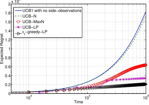
Figures 3 and 4 show the regret performance as a function of time for the two sub-networks of sizes 1000 and 2000 respectively. Note that the average regret is taken over 1000 experiments. For thet-greedy-LP policy, we letc= 5 andd= 0.2 (we choosed= 0.2

(UCB-N and UCB-MaxN policies can also be viewed as special cases of those proposed in Chen et al. (2013) for this specific combinatorial structure). We also observe that the improvement obtained by UCB-N policy over the baseline UCB1 policy is marginal. It has been shown (Cooper et al., 2005) that for power law graphs, both γ(G) and ¯χ(G) scale linearly with N, although γ(G) has a lower slope. Our numerical results show that our policies outperform existing policies even for the Flixster network.

As we show in Corollary 8 and Proposition 10,t-greedy-LP and UCB-LP have the same

upper bound O(P

j∈Uz∗jlogT). It is hard to say which algorithm outperforms the other

one. In the Flixster network, we see that the t-greedy-LP policy performs better than the

UCB-LP policy. As we show in Section 7.2, UCB-LP performs better thant-greedy-LP. In

addition, the regret gap between the t-greedy-LP and UCB-LP is not large compared to

their gain to UCB-N and UCB-maxN.

7.2 Algorithm Performance on Synthetic Data

We consider a routing problem defined on a communication network, which is demonstrated as an undirected graph consisting of 6 nodes in Figure 5. We assume that node 1 is the source node and node 6 is the destination node. The decision maker repeatedly sends packets from the source node to the destination node. There exist 13 simple paths from the source node to the destination node. The delay of each path is the sum of delays over all the constituent links. The goal of the decision maker is to identify the path with the smallest expected delay and minimize the regret as much as possible.

Solving the routing problem is a direct application of this work once we let the set of paths be the set of actions and the set of links be the set of base-arms. We assume that the delay of each link i, denoted by Xi(t), is an independent and identically distributed

sequence of random variables (drawn from the steady-state distribution) over discrete time

t. Then, this is a stochastic bandit problem with side-observations since playing one action (path) reveals some observations of some base-arms (links) that contribute to other actions (paths). For example, choosing path (1,2,4,6) reveals the delay performance of link (1,2) and (2,4), which are included in the path (1,2,4,5,6).

In the routing problem, there are 13 paths and 12 directed links (note that some links are never used in all the paths). Thus, we setK= 13 andN = 12 in the simulation. Then, we construct the set Vj for each action j such that i ∈ Vj if path j traverses the link i.

And, we set Kj = Vj for each j ∈ K since the delay of a path is the total delay of the

traversed links. Let B be the upper bound of all the action delays. Then, we choose the function fj(X~j(t)) = 1−Pi∈KjXi(t)/B as the reward of playing action j at time t. In the simulation, we assume that the delay of linkiis sampled from a Bernoulli distribution with mean ui. Each ui is independently sampled from a uniform distribution from 0 to 1,

which realizes the problem instance in Figure 53_{. One can check that the optimal action}

(shortest path) is the path (1,3,5,6) given the ground truth{ui}i∈N. We let B= 5 in the simulation.

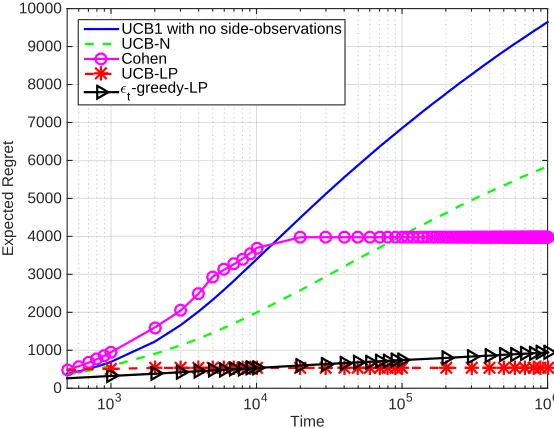
We apply the UCB1, UCB-N, Cohen (Cohen et al., 2016) and our policies to the problem instance in Figure 5 and the regret performance, averaged over 1000 experiments, is shown in Figure 6. We do not represent the result of the UCB-MaxN because it degenerates to

1  

6  

2  

3  

4  

5  

0.20  

0.35  

0.

62  

0.

75  

0.

35  

0.

55  

Figure 5: Routing problem on a communication network

Time

103 104 105 106

Expected Regret

0 1000 2000 3000 4000 5000 6000 7000 8000 9000 10000

UCB1 with no side-observations UCB-N

Cohen UCB-LP

0_t-greedy-LP

Figure 6: Regret comparison of all the policies for the routing problem

the UCB-N policy. The reason is that there is no non-trivial clique (clique with more than one element) in this problem due to the setting K_j = Vj and Kj 6= Ka for any j, a ∈ K.

Intuitively, there does not exist two paths that can observe the outcome of each other. For the t-greedy-LP policy, we let c = 4 and d = 0.05. From the regret performance, we

7.3 Asymptotic Behavior

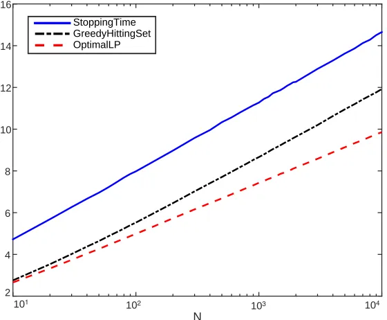
We run a simulation to verify the result provided in Proposition 5. For each base-arm size

N, we sequentially generate action j such that eij = 1 with probability p for any i ∈ N

independently. Stopping timeτ is the number of actions we have generated so that there are no useless base-arms in the network. Note that τ is an upper bound of γ(G) and P

j∈Kzj∗

as shown in Appendix B. Then, we solve the linear program P2 to obtainP

j∈Kz∗j and find

a hitting set by a greedy algorithm.4

N

2 4 6 8 10 12 14 16

StoppingTime GreedyHittingSet OptimalLP

101 102 103 104

Figure 7: Erdos-Renyi random graph with p=0.5

Figure 7 shows the average result over 1000 samples for each N when p = 0.5. The numerical result verifies our theoretical result that P

j∈Kzj∗ is upper-bounded by a

loga-rithmic function of N asymptotically in Erdos-Renyi random graph. The reason why we are interested in the scaling order of P

j∈Kzj∗ is that the traditional UCB1 policy suffers

from the curse of dimensionality when applied in the real world, such as recommendation systems with thousands of items. However, our policies show a regret ofO(P

j∈Kzj∗logT),

andP

j∈Kzj∗is upper-bounded by a logarithmic function of the number of unknowns, which

makes our policies scalable in some large networks.

8. Summary

In this work, we introduce an important structural form of feedback available in many multiarmed bandits using the bipartite network structure. We obtained an asymptotic (with respect to time) lower bound as a function of the network structure on the regret of

any uniformly good policy. Further, we proposed two policies: 1) the t-greedy-LP policy,

and 2) the UCB-LP policy, both of which are optimal in the sense that they achieve the asymptotic lower bound on the regret, up to a multiplicative constant that is independent of the network structure. These policies can have a better regret performance than existing policies for some important network structures. Thet-greedy-LP policy is a network-aware

any-time policy, but its exploration is oblivious to the average rewards of the suboptimal actions. On the other hand, UCB-LP considers both the network structure and the average rewards of actions.

In what follows, we give the proofs of all propositions stated in the earlier sections. These proofs make use of Lemmas 15, 16, and 17, and Proposition 18 given in Section F.

Appendix A. Proof of Proposition 4

Let U = {j : µj < µ∗} be the set of suboptimal actions. Also, let ∆j = µ∗ −µj. Also,

Tj(t) is the total number of times action j is chosen up to time t by policy φ. Let Mi(t)

be the total number of observations corresponding to base-arm iavailable at time t. From Proposition 18 given in the Appendix, we have,

lim inf

t→∞

E[Mi(t)]

log(t) ≥ 1

Ji(θi)

, ∀i∈ N. (8)

An observation is received for base-armiwhenever any action in Si is chosen. Hence,

Mi(t) =

X

j∈Si

Tj(t). (9)

Now, from Equations (8) and (9), for each i∈ N,

lim inf

t→∞ P

j∈SiE[Tj(t)] log(t) ≥

1

Ji(θi)

. (10)

Using (10), we get the constraints of LPP1. Further, we have from definition of regret that,

lim inf

t→∞

Rµ(t)

log(t) = lim inft→∞ X

j∈U ∆jE

[Tj(t)]

log(t) .

The above equation along with the constraints of the LP P1 obtained from (10) gives us

the required lower bound on regret.

Appendix B. Proof of Proposition 5

Here we consider a E-R random graph with each entry of the matrix E equals 1 with probability p, where 0 < p <1. Consider the following discrete stochastic process. χn are

i.i.d., such that χn⊆[N] is sampled by the following steps: for each i= 1,2, .., N,i∈χn

with probability p. Letq = 1−p. Then let τ be a stopping time defined as

τ = min{n≥1,∪_jn₌₁χj = [N]} (11)

The complement cdf ofτ is the following.

P(τ > n) = 1−(1−qn)N (12)

1. Fix N. Given 0< p <1, then 0< q <1. Thus,P(τ =∞) = 0

2. What is the upper bound ofE(τ)?

(1−qn)N >exp(− q

n_N

1−qn) (since ln(1−x)>−

x

Thus, we have

P(τ > n)<1−exp(− q

n_N

1−qn)≤

qnN

1−qn (since1−e

x_{≤ −x) (14)}

Then we can bound the expectation ofτ.

E(τ) = ∞ X

n=1

P(τ > n)<

∞ X

n=1 qn N

1−q = qN

(1−q)2 (15)

3. What is the upper bound ofP(τ ≤n)?

P(τ ≤n) = (1−qn)N ≤exp(−qnN) (16)

4. Doesτ converge asN goes to infinity? Given >0, asN goes to∞,

P(τ ≤(1−) log_1/qN)≤exp(−q(1−) log1/qN_{N) = exp(−N)→0 (17)}

P(τ >(1 +) log_1/qN)≤ q

(1+) log1/qN_N

1−q =

1

(1−q)N →0 (18)

Since is arbitrary, we can have

P(τ = log_1/qN)→1 as N → ∞. (19)

That is to say τ converges to log_1/qN in probability.

Suppose there are no useless base-arms in the network, i.e. [K] is a hitting set. Thenτ

is less than K with probability 1. Given this information, γ(G) should be upper bounded by log_1/qN asN goes to infinity.

Appendix C. Proof of Proposition 6

Let (z∗_j)j∈K be the optimal solution of LPP2.We will first prove the upper bound in Equa-tion 2. Using the optimal soluEqua-tion (w_j∗)j∈Kof LPP1,we construct a feasible solution

satisfy-ing constraints in LPP2 in the following way: For actions j∈ K,let zj =

max

i∈N Ji(θi)

w∗_j.

Then (zj)j∈K satisfy constraints for all base-arms i∈ N because wj∗ satisfy constraints of

LP P1.

The feasible solution constructed in this way gives an upper bound on the optimal value of LP P2.Hence,

X

j∈K

z∗_j ≤X

j∈U

zj +|O|

≤X

j∈U

max

i∈N Ji(θi)

w_j∗+|O|

≤ maxi∈NJi(θi)

minj∈U∆j

X

j∈U

∆jw∗j +|O|

≤ maxi∈NJi(θi)

minj∈U∆j

For the lower bound, any feasible solution ofP2,in particular z∗,can be used to construct

a feasible solution ofP1.For actionsj∈ K,let wj =

z_j∗

mini∈N Ji(θi)

.Then (wj)j∈K satisfies the constraints of LP P1 and hence gives an upper bound on its optimal value. Therefore,

we have

cµ=

X

j∈U ∆jw∗j,

≤X

j∈K

∆jz∗_j

mini∈NJi(θi)

≤X

j∈K

maxa∈U ∆azj∗

mini∈NJi(θi)

which gives us the required lower bound.

Appendix D. Proof of Proposition 7

Since z∗ satisfies the constraints in LPP2, there is sufficient exploration within each sub-optimal action’s neighborhood. The proof is then a combination of this fact and the proof of Theorem 3 in Auer et al. (2002). Let ¯fj(t) be the random variable denoting the sample

mean of all observations available for action j at timet. Let ¯f∗(t) be the random variable denoting the sample mean of all observations available for an optimal action at timet. Fix a suboptimal action j. For someα >1,define mi for each base-armias follows,

mi =

1

α

P

j∈Siz ∗

j

P

j∈Kz∗j t

X

m=1 (m)

Letφ(t) be the action chosen byt-greedy-LP policy at timet.The event{φ(t) =j}implies

that either sampling a random actionj for exploration or playing the best observed action

j for exploitation. Then,

P[φ(t) =j]≤

(t)z_j∗

P

a∈Kza∗

+ (1−(t))P[ ¯fj(t)≥f¯∗(t)]

The event{f¯j(t)≥f¯∗(t)} implies that either{f¯j(t)≥µj+∆₂j}or{f¯∗(t)≤µ∗−∆₂j}since

µj+∆₂j =µ∗−∆₂j. We also have that,

P[ ¯fj(t)≥f¯∗(t)]≤P

¯

fj(t)≥µj+

∆j

2

+P

¯

f∗(t)≤µ∗−∆j

2

.

The analysis of both the terms in the right hand side of the above expression is similar. LetOR_i (t) be the total number of observations available for base-armifrom the exploration iterations of the policy up to timet.LetOi(t) be the total number of observations available

number of observations for action j is lower-bounded by the number of observations from the exploration iterations. Hence, we have,

P

¯

fj(t)≥µj+

∆j 2 = t X m=1 P min

i∈Kj

Oi(t) =m; ¯fj(t)≥µj+

∆j 2 = t X m=1 P ¯

fj(t)≥µj+

∆j

2 |mini∈Kj

Oi(t) =m

P

min

i∈Kj

Oi(t) =m

≤ t X m=1 P min

i∈Kj

Oi(t) =m

e −∆2_{j m}

2

(follows from Chernoff-Hoeffding bound in Lemma 15)

≤ t X m=1 P min

i∈Kj

O_iR(t)≤m

e −∆2_{j m}

2

≤

bm0c X

m=1

P

min

i∈Kj

OR_i (t)≤m

+

t

X

m=bm0c+1

e −∆2_{j m}

2

≤m0P

min

i∈Kj

OR_i (t)≤m0

+ 2

∆2_je

−∆2_{j m0} 2

since ∞ X

m+1

e−ku≤ 1 ke

−km

!

≤ X

i∈Kj

m0PORi (t)≤m0

+ 2

∆2

j

e −∆2_{j m}0

2 ,

wherem0= mini∈Nmi.

Recall that O_iR(t) is the total number of observations for base-armi from exploration. Now, we derive the bounds for the expectation and variance of OR_i (t) in order to use Bernstein’s inequality.

EORi (t)

=

t

X

m=1

(m)X

j∈Si

z_j∗

P

j∈Kzj∗

= P

j∈Siz ∗

j

P

j∈Kz∗j t

X

m=1

(m) =αmi

≥αm0

var

OR_i (t) =

t

X

m=1



(m) X

j∈Si

z_j∗

P

j∈Kzj∗



 

1−(m)X

j∈Si

z_j∗

P

j∈Kz∗j

  ≤ t X m=1

(m)X

j∈Si

z∗_j

P

j∈Kzj∗

Now, using Bernstein’s inequality given in Lemma 16, we have

POiR(t)≤m0

=PORi (t)≤E[OiR(t)] +m0−αmi

≤_P

O_iR(t)≤_E[O_iR(t)] +mi−αmi

≤exp − (α−1) 2_m2

i

2αmi+2₃(α−1)mi

!

= exp

−3(α−1) 2

8α−2 mi

= exp(−rmi)

where r = 3(₈α_α−₋1)₂2.Now, we will obtain upper and lower bounds on mi by plugging in the

definition of(m). For the upper bound, for anyt > t0 = c P

i∈Kzi∗ d2 ,

mi =

P

j∈Siz ∗

j

αP

j∈Kzj∗ t

X

m=1 (m)

= P

j∈Siz ∗

j

αP

j∈Kzj∗

t0+ P

j∈Siz ∗

j

αP

j∈Kzj∗ t

X

m=t0₊₁ cP

i∈Kzi∗

d2_m ≤ cδ

αd2 1 +

t

X

m=t0₊₁

1

m

!

≤ cδ αd2log

e2t t0

.

where δ = maxi∈N|Si|, denoting the maximum degree of the supports in the network. In

the above, P

j∈Siz ∗

j ≤ δ because z

∗

j ≤ 1, which is due to the fact that

z_j∗

j∈K is the optimal solution of LPP2.Next, for the lower bound, we use the fact thatPj∈Siz

∗

j ≥1 for

all ibecause

z∗_j

j∈K satisfies the constraints of LPP2.Thus

mi ≥

P

j∈Siz ∗

j

αP

j∈Kzj∗ t

X

m=t0₊₁ cP

i∈Kzi∗

d2_m

≥ c

αd2

t

X

m=t0₊₁

1

m

≥ c

αd2 log

t et0

Letλ= maxj∈K|Kj|. Hence, combining the inequalities above,

P

¯

fj(t)≥µj+

∆j

2

≤ X

i∈Kj

m0POiR(t)≤m0

+ 2

∆2

j

e−

∆2_{j m0} 2

≤ X

i∈Kj

m0 et0 t cr/αd2 + 2

∆2_je −∆2j m₂ 0

≤λ cδ αd2

log

e2t t0

et0 t

cr/αd2

+ 2

∆2_j

et0 t

c∆2_j

2αd2

Now, similarly for the optimal action, we have, for all t > t0

P

¯

f∗_(t)≤µ∗₋∆j

2 ≤ λcδ αd2 et0 t cr/αd2 log

e2t t0

+ 2

∆2_j

et0 t

c∆2_j

2αd2

.

Combining everything, we have for any suboptimal actionj, for all t > t0

P[φ(t) =j]≤

(t)z_j∗

P

a∈Kza∗

+ (1−(t))P[ ¯fj(t)≥f¯∗(t)]

≤ cz

∗

j

d2_t +P[ ¯fj(t)≥f¯

∗_(t)]

≤ cz

∗

j

d2_t +

2λcδ αd2 et0 t cr/αd2 log

e2t t0

+ 4

∆2_j

et0 t

c∆2_j

2αd2

Appendix E. Proof of Proposition 10

The proof technique is similar to that in Auer and Ortner (2010). We will analyze the regret by conditioning on two disjoint events. The first event is that each suboptimal action ais eliminated by an optimal action on or before the first roundmsuch that ˜∆m <∆a/2.This

happens with high probability and leads to logarithmic regret. The compliment of the first event yields linear regret in time but occurs with probability proportional to 1/T.The main difference from the proof in Auer and Ortner (2010) is that on the first event, the number of times we choose each action j is proportional to z_j∗log(T) in the exploration iterations (i.e., when |Bm| > 1) of the policy. This gives us the required upper bound in terms of

optimal solution z∗ of LPP2.

Let ∗ denote any optimal action. Let m∗ denote the round in which the last optimal action ∗ is eliminated. For each suboptimal action j, define round mj := min{m : ˜∆m <

∆j

2 }.For an optimal actionj, mj =∞ by convention. Then, by the definition ofmj,for all

rounds m < mj,∆j ≤2 ˜∆m,and

2 ∆j

<2mj ₌ 1 ˜ ∆mj

≤ 4

∆j

< 1

˜ ∆mj+1

= 2mj+1_{. (20)}

From Lemma 17 in the Appendix, the probability that action j is not eliminated in round

mj by ∗ is at most _T∆˜22 mj

LetI(t) be the action chosen at timetby the UCB-LP policy.

LetEm∗ be the event that all suboptimal actions withm_j ≤m∗ are eliminated by ∗ on or

before their respectivemj. Then, the complement ofEm∗,denoted asE_mc∗,is the event that

there exists some suboptimal actionjwithmj ≤m∗,which is not eliminated by roundmj.

LetE_jcbe the event that actionj is not eliminated by roundmj by ∗.Letmf =b1₂log2 Tec

and I(t) denote the action chosen at timet by the policy. Recall that regret is denoted by

Rµ(T).LetP[m∗ =m] be denoted by pm.Hence,P mf

m=0pm= 1. E[Rµ(T)] =

mf X

m=0

E[Rµ(T)|{m∗ =m}]P[m∗=m]

= mf X m=0 T X t=1 X j∈U

∆jP[I(t) =j|{m∗=m}]pm

= mf X m=0 T X t=1 X j∈U

∆jP[{I(t) =j} ∩Em∗|{m∗ =m}]p_m

+ mf X m=0 T X t=1 X j∈U

∆jP[{I(t) =j} ∩Emc∗|{m∗=m}]pm

= (i) + (ii)

Next we will show that term (i) leads to logarithmic regret while term (ii) leads to a constant regret with time.

First, consider the term (ii) of the regret expression. For each j∈ U,we have,

mf X m=0 T X t=1

P[{I(t) =j} ∩Emc∗|{m∗ =m}]P[m∗ =m]

≤ mf X m=0 T X t=1

P[{I(t) =j} ∩(∪a∈U:ma≤m∗E c a)|{m

∗

=m}]pm

≤ mf X m=0 T X t=1

P[{I(t) =j}|(∪a∈U:ma≤m∗E c

a),{m∗ =m}]

P[∪a∈U:ma≤m∗E c a|{m

∗

=m}]pm

≤TP[∪a∈UEac|{m∗ =mf}] mf X

m=0 pm

≤TX

a∈U 2

T∆˜2

ma

,

using Lemma 17, P[Eac|{m

∗

=mf}]≤

2

T∆˜2

where the last inequality follows from Equation (20). Hence, the term (ii) of regret is

mf X

m=0

T

X

t=1

X

j∈U

∆jP[{I(t) =j} ∩Emc∗|{m∗ =m}]pm

≤X

j∈U ∆j

X

a∈U 32 ∆2

a

=O(K2). (21)

Next, we consider the term (i). Recall that, in this term, we consider the case that all suboptimal actions j withmj ≤m∗ are eliminated by∗on or before mj.

(i) =

mf X

m=0

T

X

t=1

X

j∈U

∆jP[{I(t) =j} ∩Em∗|{m∗=m}]p_m

=

mf X

m=0

E[Rµ(T)|{m∗=m}, Em∗]_P[E_m∗|{m∗ =m}]p_m

≤

mf X

m=0

E[Regret from{j:mj ≤m∗}|{m∗ =m}, Em∗]

+E[Regret from{j:mj > m∗}|{m∗ =m}, Em∗]

pm

≤

mf X

m=0

ERegret from {j:mj ≤mf}|{m∗=mf}, Emf

+E[Regret from{j:mj > m∗}|{m∗ =m}, Em∗]

pm

≤_E

Rµ(T)|{m∗=mf}, Emf

mf X

m=0 pm

+

mf X

m=0

E[Regret from{j:mj > m∗}|{m∗=m}, Em∗]p_m

= (ia) + (ib)

Once again, we will consider the above two terms separately. For the term (ia),under the eventEmf, each suboptimal actionj is eliminated by ∗by round mj. Define round ¯m and the set B as follows:

¯

m= min{m:X

j∈K

z∗_j > X

a:ma>m

2−m+1}, B ={j∈ U :mj >m¯}.

After round ¯m, Algorithm 2 chooses only those actions withmj >m.¯ Also, by the definition

first. Define nj = min{m,¯ max a:j∈Ga

{ma}} for each suboptimal action j, where Ga =Si∈KaSi for actiona. Then any suboptimal actionj /∈B is chosen for at mostnj rounds.

(ia) =ERµ(T)|{m∗ =mf}, Emf

≤ X

j∈U \B

∆jz∗j

2 log(T∆˜2_nj) ˜ ∆2

nj

+X

j∈B

∆j

2 log(T∆˜2_mj) ˜ ∆2

mj

≤ X

j∈U \B

∆jz∗j

32 log(T∆ˆ2_j) ˆ

∆2_j +

X

j∈B

∆j

32 log(T∆2_j)

∆2_j , (22)

where ˆ∆j = max{2−m¯+2,mina:j∈Ga{∆a}} and (z ∗

j) is the solution of LPP2.

Finally, we consider the term (ib).Note thatTj(m)≥n(m),∀j∈Bm,∀m.An optimal action

∗ is not eliminated in round m∗ if (25) holds form=m∗. Hence, using (26) and (27), the probability pm that ∗ is eliminated by a suboptimal action in any round m∗ is at most

2

T∆˜2 m∗

.Hence, term (ib) is given as:

mf X

m=0

E[Regret from{j:mj > m∗}|{m∗=m}, Em∗]p_m

≤

mf X

m=0

X

j∈U:mj≥m 2

T∆˜2

m

.Tmax

a∈U ∆a

≤max

a∈U ∆a

mf X

m=0

X

j∈U:mj≥m 2 ˜ ∆2 m ≤X j∈U mj X m=0 2 ˜ ∆2 m ≤X j∈U

22mj+2_≤X j∈U

64 ∆2

j

=O(K). (23)

Now we get the result (6) by combining the bounds in (21), (22), and (23). Further, the definition of setB ensures that we have

X

j∈B

∆j ≤

X

j∈K

z∗_j.

Also, using the Assumption 4, 32∆jlog(T∆ˆ 2 j)

ˆ ∆2

j

,32 log(T∆

2 j)

∆2 j

are bounded by Clog(T), where

C = _min32 j∈U∆2j

, is a constant independent of network structure. When one checks the

rewards are bounded by 1. Hence, (22) can be bounded as:

X

j∈U \B

∆jzj∗

32 log(T∆ˆ2_j) ˆ

∆2_j +

X

j∈B

∆j

32 log(T∆2_j) ∆2_j

≤ X

j∈U \B

z_j∗Clog(T) +X

j∈B

∆jClog(T)

≤ X

j∈U \B

z_j∗Clog(T) +X

j∈B

2−m¯+1Clog(T)

≤2X

j∈K

z_j∗Clog(T). (24)

Hence, we get (7) from (24), (21), and (23).

Appendix F. Supplementary Material

Sn = _n1 Pn_j=1Xj denotes the sample mean of the random variables X1, . . . , Xn. The first

two lemmas below state the Chernoff-Hoeffding inequality and Bernstein’s inequality.

Lemma 15 LetX1, . . . , Xnbe a sequence of random variables with support[0,1]andE[Xt] =

µ for allt≤n. Let Sn= 1_n

Pn

j=1Xj.Then, for all >0,we have, P[Sn≥µ+]≤e−2n

2

P[Sn≤µ−]≤e−2n

2

.

Lemma 16 LetX1, . . . , Xnbe a sequence of random variables with support[0,1]and

Pt k=1 var[Xk|X1, . . . , Xk−1]≤σ2 for all t≤n. Let Sn=Pnj=1Xj.Then, for all >0, we have,

P[Sn≥E[Sn] +]≤exp

(

−

2

2σ2₊2 3

)

P[Sn≤E[Sn]−]≤exp

(

−

2

2σ2₊2 3

)

.

The next lemma is used in the proof of Proposition 10.

Lemma 17 The probability that action j is not eliminated in round mj by ∗ is at most

2

T∆˜2 mj

.

Proof Let ¯fj(m) be the sample mean of all observations for actionj available in roundm.

Let ¯f∗(m) be the sample mean of the optimal action. The constraints of LPP2 ensure that at the end of each round m, for all actions in Bm, we have at least n(m) :=

l

2 log(T∆˜2m)

˜ ∆2

m m

observations. The reason is as follows. The set Am contains set Bm. In particular, Am =

∪i∈DmSi and Dm = ∪j∈BmKj. If each action j in Am is played z ∗

j times, then all the

the actions in Bm have at least 1 observations. In sum, for all actions in Bm, we have at

leastn(m)−n(m−1) observations at round m. Thus, we have at leastn(m) observations for all actions inBm.

Now, for m=mj,if we have,

¯

fj(m)≤µj +

s

log(T∆˜2

m)

2n(m) and ¯f ∗

(m)≥µ∗−

s

log(T∆˜2

m)

2n(m) , (25)

then, action j is eliminated by∗ in roundmj.In fact, in round mj,we have

s

log(T∆˜2

mj) 2n(mj)

≤

˜ ∆mj

2 < ∆j

4 .

Hence, in the elimination phase of the UCB-LP policy, if (25) holds for action j in round

mj,we have,

¯

fj(mj) +

s

log(T∆˜2

mj) 2n(mj)

≤µj + 2

s

log(T∆˜2

mj) 2n(mj)

< µj + ∆j−2

s

log(T∆˜2

mj) 2n(mj)

=µ∗−2 s

log(T∆˜2

mj) 2n(mj)

≤f¯∗(mj)−

s

log(T∆˜2

mj) 2n(mj)

,

and actionj is eliminated. Hence, the probability that action j is not eliminated in round

mj is the probability that either one of the inequalities in (25) do not hold. Using

Chernoff-Hoeffding bound (Lemma 15), we can bound this as follows,

P



f¯_j(m)> µ_j+ s

log(T∆˜2

m)

2n(m) 

≤ 1

T∆˜2

m

(26)

P



f¯∗(m)< µ∗− s

log(T∆˜2

m)

2n(m) 

≤ 1

T∆˜2

m

. (27)

Summing the above two inequalities form=mj gives us that the probability that actionj

is not eliminated in round mj by ∗ is at most _T∆˜22 mj

.

The next proposition is a modified version of Theorem 2 in Lai and Robbins (1985). We use it to obtain the regret lower bound in Proposition 4.

Proposition 18 Suppose Assumptions 1, 2, and 3 hold. Let Mi(t) be the total number of

observations for such a base-armi,for which~θ∈Θi.Then, under any uniformly good policy

φ, we have that

lim inf

t→∞

E[Mi(t)]

log(t) ≥ 1

Ji(θi)

Proof By definition ofJi(θi),for every >0,there exists aθ0i ∈ Bi(θi) such thatJi(θi)<

D(θi||θ0i)<(1 +)Ji(θi).

Now, under ~θ_i0 = [θ1, . . . , θ_i0, . . . θN], there exists an action k ∈ Si such that k is the

unique optimal action. Then, for any uniformly good policy, for 0< b < δ,

E~_θ0

i[t

−Tk(t)] =o(tb)

and therefore,

P~_θ0

i

Tk(t)<(1−δ) log(t)/D(θi||θi0)

=o(tb−1),

similar to the asymptotic lower bound proof in Lai and Robbins (1985).

LetMi(t) be the total number of observations for base-armi.ThenMi(t)≥Tk(t),since

choosing any action in Si gives observations for i.Hence,

P~_θ0

i

Mi(t)<(1−δ) log(t)/D(θi||θi0)

=o(tb−1),

Now the rest of the proof of Theorem 2 in Lai and Robbins (1985) applies directly toMi(t).

We will repeat it below for completeness. Let (Yi(r))r≥1 be the observations drawn from

distributionFi and define

Lm= m

X

r=1

log

g(Yi(r);θi)

g(Yi(r);θ0_i)

.

Now, we have thatP~_θ0

i

[Ct] =o(tb−1) whereCt={Mi(t)<(1−δ) log(t)/D(θi||θi0) and LMi(t) ≤ (1−b) log(t)}.

Now, we use the change of measure arguments.

P_θ~0

i

[M1(t) =m1, . . . , MN(t) =mN, Lmi ≤(1−b) log(t)] (28) =

Z

{M1(t)=m1,...,MN(t)=mN,Lmi≤(1−b) log(t)} Πmi

r=1

g(Yi(r);θ_i0)

g(Yi(r);θi)

dP_θ~_i (29)

≥exp(−(1−b) log(t))P_θ~_i[M1(t) =m1, . . . , MN(t) =mN, Lmi ≤(1−b) log(t)] (30) Since Ct is a disjoint union of events of the form {M1(t) = m1, . . . , MN(t) = mN, Lmi ≤ (1−b) log(t)} withmi<(1−δ) log(t)/D(θi||θ0i), it follows that

P~_θ[Ct]≤t1−bP~_θ0

i

[Ct]→0.

So far, we show that the probability of the event Ct goes to 0 as t goes to infinity. If

we show the event {LMi(t) ≤(1−b) log(t)|Mi(t) <(1−δ) log(t)/D(θi||θ 0

i)} occurs almost

surely, then we show the probability of{Mi(t)<(1−δ) log(t)/D(θi||θi0)}goes to 0 astgoes

to infinity, which is the desired result. By strong law of large numbers Lm/m→ D(θi||θ0i)

asm→ ∞and maxr≤mLr/m→D(θi||θi0) almost surely. Now, since 1−b >1−δ,it follows

that as t→ ∞,

P~_θLr>(1−b) log(t) for somer <(1−δ) log(t)/D(θi||θi0)

→0. (31)

Hence, we have that as t→ ∞,

P~_θMi(t)<(1−δ) log(t)/D(θi||θi0)

By choosing, δ appropriately, this translates to

lim inf

t→∞

E[Mi(t)]

log(t) ≥ 1

Ji(θi)

.

Proposition 19 When the horizon is unknown, start the UCB-LP algorithm with T0˜ = 2

and increaseT˜ after reachingT˜ steps by setting T˜l+1= ˜Tl2. The regret of unknown horizon

UCB-LP is bounded by

X

j∈U \B

64∆jzj∗

ˆ

∆2_j log(T ˆ

∆2_j) +X

j∈B

64 log(T∆2_j) ∆j

+O(K2log₂log₂T). (32)

Proof When the horizon is unknown, start the UCB-LP algorithm with ˜T0 = 2 and increase

˜

T after reaching ˜T steps by setting ˜Tl+1 = ˜T_l2. Thus, ˜Tl = 22 l

until reaching horizon T. Also, the period in which horizon is reached is denoted by L. Note that 2≤L≤log₂log₂T. In any period l,(0≤l≤L), UCB-LP uses ˜Tl as input. Note that ¯m, mj, B and ˆ∆j are

independent of ˜Tl, thus l. Recall that regret of UCB-LP is bounded by (6). The regret of

UCB-LP with unknown horizon is upper bounded by the summation over all the periods.

L X l=0   X

j∈U \B

∆jzj∗

32 log( ˜Tl∆ˆ2j)

ˆ

∆2_j +

X

j∈B

32 log( ˜Tl∆2j)

∆j

+O(K2) 

= (i) + (ii) + (iii).

First, we consider the term (i). We can plug in the definition of ˜Tl into (i).

(i) =

L

X

l=0

X

j∈U \B

∆jz∗j

32 log( ˜Tl∆ˆ2j)

ˆ ∆2_j

= X

j∈U \B

32∆jz∗j

ˆ ∆2 j L X l=0

log(22l∆ˆ2_j)

= X

j∈U \B

32∆jz∗j

ˆ

∆2_j (log 2)

L

X

l=0

2l+ (L+ 1) log ˆ∆2_j !

≤ X

j∈U \B

32∆jz∗j

ˆ ∆2

j

2L+1(log 2) + (L+ 1) log ˆ∆2_j

≤ X

j∈U \B

32∆jz∗j

ˆ ∆2

j

2 logT + (L+ 1) log ˆ∆2_j

(since L≤log₂log₂T)

≤ X

j∈U \B

64∆jz∗j

ˆ ∆2

j