Optimal Distributed Online Prediction Using Mini-Batches
Ofer Dekel [email protected]
Ran Gilad-Bachrach [email protected]
Microsoft Research 1 Microsoft Way
Redmond, WA 98052, USA
Ohad Shamir [email protected]
Microsoft Research 1 Memorial Drive
Cambridge, MA 02142, USA
Lin Xiao [email protected]
Microsoft Research 1 Microsoft Way
Redmond, WA 98052, USA
Editor: Tong Zhang
Abstract
Online prediction methods are typically presented as serial algorithms running on a single proces-sor. However, in the age of web-scale prediction problems, it is increasingly common to encounter situations where a single processor cannot keep up with the high rate at which inputs arrive. In this work, we present the distributed mini-batch algorithm, a method of converting many serial gradient-based online prediction algorithms into distributed algorithms. We prove a regret bound for this method that is asymptotically optimal for smooth convex loss functions and stochastic in-puts. Moreover, our analysis explicitly takes into account communication latencies between nodes in the distributed environment. We show how our method can be used to solve the closely-related distributed stochastic optimization problem, achieving an asymptotically linear speed-up over mul-tiple processors. Finally, we demonstrate the merits of our approach on a web-scale online predic-tion problem.
Keywords: distributed computing, online learning, stochastic optimization, regret bounds, convex
optimization
1. Introduction
First, we begin by defining the stochastic online prediction problem. Suppose that we observe a stream of inputs z1,z2, . . ., where each ziis sampled independently from a fixed unknown distribution
over a sample space
Z. Before observing each z
i, we predict a point wifrom a set W . After makingthe prediction wi, we observe zi and suffer the loss f(wi,zi), where f is a predefined loss function.
Then we use zito improve our prediction mechanism for the future (e.g., using a stochastic gradient
method). The goal is to accumulate the smallest possible loss as we process the sequence of inputs. More specifically, we measure the quality of our predictions using the notion of regret, defined as
R(m) =
m
∑
i=1
(f(wi,zi)−f(w⋆,zi)),
where w⋆=arg minw∈WEz[f(w,z)]. Regret measures the difference between the cumulative loss of
our predictions and the cumulative loss of the fixed predictor w⋆, which is optimal with respect to the underlying distribution. Since regret relies on the stochastic inputs zi, it is a random variable. For
simplicity, we focus on bounding the expected regretE[R(m)], and later use these results to obtain high-probability bounds on the actual regret. In this paper, we restrict our discussion to convex prediction problems, where the loss function f(w,z) is convex in w for every z∈
Z, and W is a
closed convex subset ofRn.Before continuing, we note that the stochastic online prediction problem is closely related, but not identical, to the stochastic optimization problem (see, e.g., Wets, 1989; Birge and Louveaux, 1997; Nemirovski et al., 2009). The main difference between the two is in their goals: in stochastic optimization, the goal is to generate a sequence w1,w2, . . .that quickly converges to the minimizer
of the function F(·) =Ez[f(·,z)]. The motivating application is usually a static (batch) problem, and
not an online process that occurs over time. Large-scale static optimization problems can always be solved using a serial approach, at the cost of a longer running time. In online prediction, the goal is to generate a sequence of predictions that accumulates a small loss along the way, as measured by regret. The relevant motivating application here is providing a real-time service to users, so our algorithm must keep up with the inputs as they arrive, and we cannot choose to slow down. In this sense, distributed computing is critical for large-scale online prediction problems. Despite these important differences, our techniques and results can be readily adapted to the stochastic online optimization setting.
We model our distributed computing system as a set of k nodes, each of which is an indepen-dent processor, and a network that enables the nodes to communicate with each other. Each node receives an incoming stream of examples from an outside source, such as a load balancer/splitter. As in the real world, we assume that the network has a limited bandwidth, so the nodes cannot sim-ply share all of their information, and that messages sent over the network incur a non-negligible latency. However, we assume that network operations are non-blocking, meaning that each node can continue processing incoming traffic while network operations complete in the background.
the network. We call this the no-communication solution. The main disadvantage of this solution is that the performance guarantee, as measured by regret, scales poorly with the network size k. More specifically, assuming that each node processes m/k inputs, the expected regret per node is O(p
m/k). Therefore, the total regret across all k nodes is O(√km)- namely, a factor of√k worse than the ideal solution. The first sanity-check that any distributed online prediction algorithm must pass is that it outperforms the na¨ıve no-communication solution.
In this paper, we present the distributed mini-batch (DMB) algorithm, a method of converting any serial gradient-based online prediction algorithm into a parallel or distributed algorithm. This method has two important properties:
• It can use any gradient-based update rule for serial online prediction as a black box, and convert it into a parallel or distributed online prediction algorithm.
• If the loss function f(w,z)is smooth in w (see the precise definition in Equation (5)), then our method attains an asymptotically optimal regret bound of O(√m). Moreover, the coefficient of the dominant term√m is the same as in the serial bound, and independent of k and of the network topology.
The idea of using mini-batches in stochastic and online learning is not new, and has been previously explored in both the serial and parallel settings (see, e.g., Shalev-Shwartz et al., 2007; Gimpel et al., 2010). However, to the best of our knowledge, our work is the first to use this idea to obtain such strong results in a parallel and distributed learning setting (see Section 7 for a comparison to related work).
Our results build on the fact that the optimal regret bound for serial stochastic gradient-based prediction algorithms can be refined if the loss function is smooth. In particular, it can be shown that the hidden coefficient in the O(√m) notation is proportional to the standard deviation of the stochastic gradients evaluated at each predictor wi (Juditsky et al., 2011; Lan, 2009; Xiao, 2010).
We make the key observation that this coefficient can be effectively reduced by averaging a mini-batch of stochastic gradients computed at the same predictor, and this can be done in parallel with simple network communication. However, the non-negligible communication latencies prevent a straightforward parallel implementation from obtaining the optimal serial regret bound.1 In order to close the gap, we show that by letting the mini-batch size grow slowly with m, we can attain the optimal O(√m)regret bound, where the dominant term of order√m is independent of the number of nodes k and of the latencies introduced by the network.
The paper is organized as follows. In Section 2, we present a template for stochastic gradient-based serial prediction algorithms, and state refined variance-gradient-based regret bounds for smooth loss functions. In Section 3, we analyze the effect of using mini-batches in the serial setting, and show that it does not significantly affect the regret bounds. In Section 4, we present the DMB algorithm, and show that it achieves an asymptotically optimal serial regret bound for smooth loss functions. In Section 5, we show that the DMB algorithm attains the optimal rate of convergence for stochastic optimization, with an asymptotically linear speed-up. In Section 6, we complement our theoretical results with an experimental study on a realistic web-scale online prediction problem. While sub-stantiating the effectiveness of our approach, our empirical results also demonstrate some interesting
1. For example, if the network communication operates over a minimum-depth spanning tree and the diameter of the network scales as log(k), then we can show that a straightforward implementation of the idea of parallel variance reduction leads to an O pm log(k)
Algorithm 1: Template for a serial first-order stochastic online prediction algorithm. for j=1,2, . . .do
predict wj
receive input zjsampled i.i.d. from unknown distribution
suffer loss f(wj,zj)
define gj=∇wf(wj,zj)
compute(wj+1,aj+1) =φ(aj,gj,αj) end
properties of mini-batching that are not reflected in our theory. We conclude with a comparison of our methods to previous work in Section 7, and a discussion of potential extensions and future re-search in Section 8. The main topics presented in this paper are summarized in Dekel et al. (2011). Dekel et al. (2011) also present robust variants of our approach, which are resilient to failures and node heterogeneity in an asynchronous distributed environment.
2. Variance Bounds for Serial Algorithms
Before discussing distributed algorithms, we must fully understand the serial algorithms on which they are based. We focus on gradient-based optimization algorithms that follow the template out-lined in Algorithm 1. In this template, each prediction is made by an unspecified update rule:
(wj+1,aj+1) =φ(aj,gj,αj). (1)
The update rule φtakes three arguments: an auxiliary state vector aj that summarizes all of the
necessary information about the past, a gradient gj of the loss function f(·,zj)evaluated at wj, and
an iteration-dependent parameterαj such as a stepsize. The update rule outputs the next
predic-tor wj+1∈W and a new auxiliary state vector aj+1. Plugging in different update rules results in
different online prediction algorithms. For simplicity, we assume for now that the update rules are deterministic functions of their inputs.
As concrete examples, we present two well-known update rules that fit the above template. The first is the projected gradient descent update rule,
wj+1=πW
wj−
1
αj
gj
, (2)
whereπW denotes the Euclidean projection onto the set W . Here 1/αj is a decaying learning rate,
withαj typically set to beΘ(√j). This fits the template in Algorithm 1 by defining aj to simply
be wj, and defining φto correspond to the update rule specified in Equation (2). We note that the
projected gradient method is a special case of the more general class of mirror descent algorithms (e.g., Nemirovski et al., 2009; Lan, 2009), which all fit in the template of Equation (1).
Another family of update rules that fit in our setting is the dual averaging method (Nesterov, 2009; Xiao, 2010). A dual averaging update rule takes the form
wj+1=arg min w∈W
(* j
∑
i=1
gi,w
+
+αjh(w)
)
whereh·,·idenotes the vector inner product, h : W→Ris a strongly convex auxiliary function, and
αj is a monotonically increasing sequence of positive numbers, usually set to beΘ(√j). The dual
averaging update rule fits the template in Algorithm 1 by defining ajto be∑ij=1gi. In the special case
where h(w) = (1/2)kwk22, the minimization problem in Equation (3) has the closed-form solution
wj+1=πW −
1
αj
j
∑
i=1
gj
!
. (4)
For stochastic online prediction problems with convex loss functions, both of these update rules have expected regret bound of O(√m). In general, the coefficient of the dominant √m term is proportional to an upper bound on the expected norm of the stochastic gradient (e.g., Zinkevich, 2003). Next we present refined bounds for smooth convex loss functions, which enable us to develop optimal distributed algorithms.
2.1 Optimal Regret Bounds for Smooth Loss Functions
As stated in the introduction, we assume that the loss function f(w,z)is convex in w for each z∈
Z
and that W is a closed convex set. We usek·kto denote the Euclidean norm inRn. For convenience, we use the notation F(w) =Ez[f(w,z)]and assume w⋆=arg minw∈WF(w)always exists. Our mainresults require a couple of additional assumptions:
• Smoothness - we assume that f is L-smooth in its first argument, which means that for any z∈
Z
, the function f(·,z)has L-Lipschitz continuous gradients. Formally,∀z∈
Z
, ∀w,w′∈W, k∇wf(w,z)−∇wf(w′,z)k ≤Lkw−w′k. (5)• Bounded Gradient Variance - we assume that∇wf(w,z)has aσ2-bounded variance for any
fixed w, when z is sampled from the underlying distribution. In other words, we assume that there exists a constantσ≥0 such that
∀w∈W, Ez
h
∇wf(w,z)−∇F(w)]
2i
≤σ2.
Using these assumptions, regret bounds that explicitly depend on the gradient variance can be established (Juditsky et al., 2011; Lan, 2009; Xiao, 2010). In particular, for the projected stochastic gradient method defined in Equation (2), we have the following result:
Theorem 1 Let f(w,z)be an L-smooth convex loss function in w for each z∈
Z
and assume that the stochastic gradient ∇wf(w,z) has σ2-bounded variance for all w∈W . In addition, assumethat W is convex and bounded, and let D=p
maxu,v∈Wku−vk2/2. Then usingαj=L+ (σ/D)√j
in Equation (2) gives
E[R(m)] ≤ F(w1)−F(w⋆)
+D2L+2Dσ√m.
In the above theorem, the assumption that W is a bounded set does not play a critical role. Even if the learning problem has no constraints on w, we could always confine the search to a bounded set (say, a Euclidean ball of some radius) and Theorem 1 guarantees an O(√m)regret compared to the optimum within that set.
Theorem 2 Let f(w,z)be an L-smooth convex loss function in w for each z∈
Z
, assume that the stochastic gradient ∇wf(w,z) has σ2-bounded variance for all w ∈ W , and let D =p
h(w⋆)−min
w∈Wh(w). Then, by setting w1=arg minw∈Wh(w) andαj =L+ (σ/D)√j in the
dual averaging method we have
E[R(m)] ≤ F(w1)−F(w⋆)
+D2L+2Dσ√m.
For both of the above theorems, if∇F(w⋆) =0 (which is certainly the case if W=Rn), then the expected regret bounds can be simplified to
E[R(m)] ≤ 2D2L+2Dσ√m. (6) Proofs for these two theorems, as well as the above simplification, are given in Appendix A. Al-though we focus on expected regret bounds here, our results can equally be stated as high-probability bounds on the actual regret (see Appendix B for details).
In both Theorem 1 and Theorem 2, the parametersαj are functions ofσ. It may be difficult to
obtain precise estimates of the gradient variance in many concrete applications. However, note that any upper bound on the variance suffices for the theoretical results to hold, and identifying such a bound is often easier than precisely estimating the actual variance. A loose bound on the variance will increase the constants in our regret bounds, but will not change its qualitative O(√m)rate.
Euclidean gradient descent and dual averaging are not the only update rules that can be plugged into Algorithm 1. The analysis in Appendix A (and Appendix B) actually applies to a much larger class of update rules, which includes the family of mirror descent updates (Nemirovski et al., 2009; Lan, 2009) and the family of (non-Euclidean) dual averaging updates (Nesterov, 2009; Xiao, 2010). For each of these update rules, we get an expected regret bound that closely resembles the bound in Equation (6).
Similar results can also be established for loss functions of the form f(w,z) +Ψ(w), where
Ψ(w) is a simple convex regularization term that is not necessarily smooth. For example, setting
Ψ(w) =λkwk1 with λ>0 promotes sparsity in the predictor w. To extend the dual averaging
method, we can use the following update rule in Xiao (2010):
wj+1=arg min w∈W
(*
1 j
j
∑
i=1
gi,w
+
+Ψ(w) +αj j h(w)
)
.
Similar extensions to the mirror descent method can be found in, for example, Duchi and Singer (2009). Using these composite forms of the algorithms, the same regret bounds as in Theorem 1 and Theorem 2 can be achieved even ifΨ(w) is nonsmooth. The analysis is almost identical to Appendix A by using the general framework of Tseng (2008).
Asymptotically, the bounds we presented in this section are only controlled by the varianceσ2 and the number of iterations m. Therefore, we can think of any of the bounds mentioned above as an abstract functionψ(σ2,m), which we assume to be monotonically increasing in its arguments. 2.2 Analyzing the No-Communication Parallel Solution
Using the abstract notationψ(σ2,m)for the expected regret bound simplifies our presentation
Algorithm 2: Template for a serial mini-batch algorithm. for j=1,2, . . .do
initialize ¯gj:=0 for s=1, . . . ,b do
define i := (j−1)b+s predict wj
receive input zisampled i.i.d. from unknown distribution
suffer loss f(wj,zi)
gi:=∇wf(wj,zi)
¯
gj:=g¯j+ (1/b)gi end
set(wj+1,aj+1) =φ aj,g¯j,αj
end
In the na¨ıve no-communication solution, each of the k nodes in the parallel system applies the same serial update rule to its own substream of the high-rate inputs, and no communication takes place between them. If the total number of examples processed by the k nodes is m, then each node processes at most⌈m/k⌉ inputs. The examples received by each node are i.i.d. from the original distribution, with the same variance boundσ2 for the stochastic gradients. Therefore, each node suffers an expected regret of at mostψ(σ2,⌈m/k⌉)on its portion of the input stream, and the total
regret bound is obtain by simply summing over the k nodes, that is,
E[R(m)] ≤ kψσ2,lm
k
m
.
Ifψ(σ2,m) =2D2L+2Dσ√m, as in Equation (6), then the expected total regret is
E[R(m)] ≤ 2kD2L+2Dσk
r lm
k
m
.
Comparing this bound to 2D2L+2Dσ√m in the ideal serial solution, we see that it is approximately √
k times worse in its leading term. This is the price one pays for the lack of communication in the distributed system. In Section 4, we show how this√k factor can be avoided by our DMB approach.
3. Serial Online Prediction using Mini-Batches
The expected regret bounds presented in the previous section depend on the variance of the stochas-tic gradients. The explicit dependency on the variance naturally suggests the idea of using averaged gradients over mini-batches to reduce the variance. Before we present the distributed mini-batch algorithm in the next section, we first analyze a serial mini-batch algorithm.
algorithm calculates and accumulates gradients and defines the average gradient
¯ gj=
1 b
b
∑
s=1
∇wf(wj,z(j−1)b+s).
Hence, each batch of b inputs generates a single average gradient. Once a batch ends, the serial mini-batch algorithm feeds ¯gjto the update ruleφas the jthgradient and obtains the new prediction
for the next batch and the new state. See Algorithm 2 for a formal definition of the serial mini-batch algorithm. The appeal of the serial mini-batch setting is that the update rule is used less frequently, which may have computational benefits.
Theorem 3 Let f(w,z)be an L-smooth convex loss function in w for each z∈
Z
and assume that the stochastic gradient∇wf(w,zi)hasσ2-bounded variance for all w. If the update ruleφhas theserial regret boundψ(σ2,m), then the expected regret of Algorithm 2 over m inputs is at most
bψ
σ2
b ,
lm
b
m
.
Ifψ(σ2,m) =2D2L+2Dσ√m, then the expected regret is bounded by
2bD2L+2Dσ√m+b.
Proof Assume without loss of generality that b divides m, and that the serial mini-batch algorithm
processes exactly m/b complete batches.2Let
Z
bdenote the set of all sequences of b elements fromZ, and assume that a sequence is sampled from
Z
b by sampling each element i.i.d. fromZ. Let
¯
f : W×
Z
b7→Rbe defined as¯
f(w,(z1, . . . ,zb)) =
1 b
b
∑
s=1
f(w,zs).
In other words, ¯f averages the loss function f across b inputs from
Z, while keeping the prediction
constant. It is straightforward to show thatE¯z∈Zbf¯(w,¯z) =Ez∈Zf(w,z) =F(w).Using the linearity of the gradient operator, we have
∇wf¯(w,(z1, . . . ,zb)) =
1 b
b
∑
s=1
∇wf(w,zs) .
Let ¯zj denote the sequence(z(j−1)b+1, . . . ,zjb), namely, the sequence of b inputs in batch j. The
vector ¯gj in Algorithm 2 is precisely the gradient of ¯f(·,¯zj) evaluated at wj. Therefore the serial
mini-batch algorithm is equivalent to using the update ruleφwith the loss function ¯f .
Next we check the properties of ¯f(w,¯z)against the two assumptions in Section 2.1. First, if f is L-smooth then ¯f is L-smooth as well due to the triangle inequality. Then we analyze the variance of the stochastic gradient. Using the properties of the Euclidean norm, we can write
∇wf¯(w,¯z)−∇F(w)
2
=
1 b
b
∑
s=1
(∇wf(w,zs)−∇F(w))
2
= 1 b2
b
∑
s=1 b
∑
s′=1
D
∇wf(w,zs)−∇F(w),∇wf(w,zs′)−∇F(w)
E
.
Notice that zsand zs′ are independent whenever s6=s′, and in such cases,
E
D
∇wf(w,zs)−∇F(w),∇wf(w,zs′)−∇F(w)
E
= DE∇
wf(w,zs)−∇F(w)
,E∇
wf(w,zs′)−∇F(w)
E
= 0.
Therefore, we have for every w∈W ,
E∇wf¯(w,¯z)−∇F(w)
2
= 1 b2
b
∑
s=1
E(∇wf(w,zs)−∇F(w))
2
≤ σ
2
b . (7)
So we conclude that∇wf¯(w,¯zj)has a(σ2/b)-bounded variance for each j and each w∈W . If the
update ruleφhas a regret boundψ(σ2,m)for the loss function f over m inputs, then its regret for ¯f
over m/b batches is bounded as
E
m/b
∑
j=1
¯
f(wj,¯zj)−f¯(w⋆,¯zj)
≤ ψ
σ2
b , m b
.
By replacing ¯f above with its definition, and multiplying both sides of the above inequality by b, we have
E
m/b
∑
j=1 jb
∑
i=(j−1)b+1
f(wj,zi)−f(w⋆,zi)
≤ bψ
σ2
b , m
b
.
Ifψ(σ2,m) =2D2L+2Dσ√m, then simply plugging in the general bound bψ(σ2
/b,⌈m/b⌉)and
using ⌈m/b⌉ ≤m/b+1 gives the desired result. However, we note that the optimal algorithmic
pa-rameters, as specified in Theorem 1 and Theorem 2, must be changed toαj=L+ (σ/√bD)√j to
reflect the reduced varianceσ2/b in the mini-batch setting.
The bound in Theorem 3 is asymptotically equivalent to the 2D2L+2Dσ√m regret bound for
the basic serial algorithms presented in Section 2. In other words, performing the mini-batch update in the serial setting does not significantly hurt the performance of the update rule. On the other hand, it is also not surprising that using mini-batches in the serial setting does not improve the regret bound. After all, it is still a serial algorithm, and the bounds we presented in Section 2.1 are optimal. Nevertheless, our experiments demonstrate that in real-world scenarios, mini-batching can in fact have a very substantial positive effect on the transient performance of the online prediction algorithm, even in the serial setting (see Section 6 for details). Such positive effects are not captured by our asymptotic, worst-case analysis.
4. Distributed Mini-Batch for Stochastic Online Prediction
through other nodes. The latency incurred between u and v is therefore proportional to the graph distance between them, and the longest possible latency is thus proportional to the diameter of
G
.In addition to latency, we assume that the network has limited bandwidth. However, we would like to avoid the tedious discussion of data representation, compression schemes, error correcting, packet sizes, etc. Therefore, we do not explicitly quantify the bandwidth of the network. Instead, we require that the communication load at each node remains constant, and does not grow with the number of nodes k or with the rate at which the incoming functions arrive.
Although we are free to use any communication model that respects the constraints of our net-work, we assume only the availability of a distributed vector-sum operation. This is a standard3 synchronized network operation. Each vector-sum operation begins with each node holding a vec-tor vj, and ends with each node holding the sum∑kj=1vj. This operation transmits messages along a
rooted minimum-depth spanning-tree of
G
, which we denote byT
: first the leaves ofT
send their vectors to their parents; each parent sums the vectors received from his children and adds his own vector; the parent then sends the result to his own parent, and so forth; ultimately the sum of all vectors reaches the tree root; finally, the root broadcasts the overall sum down the tree to all of the nodes.An elegant property of the vector-sum operation is that it uses each up-link and each down-link in
T
exactly once. This allows us to start vector-sum operations back-to-back. These vector-sum operations will run concurrently without creating network congestion on any edge ofT
. Further-more, we assume that the network operations are non-blocking, meaning that each node can continue processing incoming inputs while the vector-sum operation takes place in the background. This is a key property that allows us to efficiently deal with network latency. To formalize how latency affects the performance of our algorithm, let µ denote the number of inputs that are processed by the entire system during the period of time it takes to complete a vector-sum operation across the entire network. Usually µ scales linearly with the diameter of the network, or (for appropriate network architectures) logarithmically in the number of nodes k.4.1 The DMB Algorithm
We are now ready to present a general technique for applying a deterministic update rule φin a distributed environment. This technique resembles the serial mini-batch technique described earlier, and is therefore called the distributed mini-batch algorithm, or DMB for short.
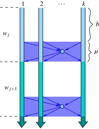
Algorithm 3 describes a template of the DMB algorithm that runs in parallel on each node in the network, and Figure 1 illustrates the overall algorithm work-flow. Again, let b be a batch size, which we will specify later on, and for simplicity assume that k divides b and µ. The DMB algorithm processes the input stream in batches j=1,2, . . ., where each batch contains b+µ consecutive inputs. During each batch j, all of the nodes use a common predictor wj. While observing the first b
inputs in a batch, the nodes calculate and accumulate the stochastic gradients of the loss function f at wj. Once the nodes have accumulated b gradients altogether, they start a distributed vector-sum
operation to calculate the sum of these b gradients. While the vector-sum operation completes in the background, µ additional inputs arrive (roughly µ/k per node) and the system keeps processing them using the same predictor wj. The gradients of these additional µ inputs are discarded (to this
end, they do not need to be computed). Although this may seem wasteful, we show that this waste can be made negligible by choosing b appropriately.
Algorithm 3: Distributed mini-batch (DMB) algorithm (running on each node). for j=1,2, . . .do
initialize ˆgj:=0 for s=1, . . . ,b/k do
predict wj
receive input z sampled i.i.d. from unknown distribution suffer loss f(wj,z)
compute g :=∇wf(wj,z)
ˆ
gj:=gˆj+g end
call the distributed vector-sum to compute the sum of ˆgj across all nodes
receive µ/k additional inputs and continue predicting using wj
finish vector-sum and compute average gradient ¯gjby dividing the sum by b
set(wj+1,aj+1) =φ aj,g¯j,αj
end
1 2 . . . k
wj
wj+1
b
µ
Figure 1: Work flow of the DMB algorithm. Within each batch j=1,2, . . ., each node accumulates the stochastic gradients of the first b/k inputs. Then a vector-sum operation across the network is used to compute the average across all nodes. While the vector-sum operation completes in the background, a total of µ inputs are processed by the processors using the same predictor wj, but their gradients are not collected. Once all of the nodes have the
overall average ¯gj, each node updates the predictor using the same deterministic serial
Once the vector-sum operation completes, each node holds the sum of the b gradients collected during batch j. Each node divides this sum by b and obtains the average gradient, which we denote by ¯gj. Each node feeds this average gradient to the update ruleφ, which returns a new synchronized
prediction wj+1. In summary, during batch j each node processes(b+µ)/k inputs using the same
predictor wj, but only the first b/k gradients are used to compute the next predictor. Nevertheless,
all b+µ inputs are counted in our regret calculation.
If the network operations are conducted over a spanning tree, then an obvious variants of the DMB algorithm is to let the root apply the update rule to get the next predictor, and then broadcast it to all other nodes. This saves repeated executions of the update rule at each node (but requires interruption or modification of the standard vector-sum operations in the network communication model). Moreover, this guarantees all the nodes having the same predictor even with update rules that depends on some random bits.
Theorem 4 Let f(w,z)be an L-smooth convex loss function in w for each z∈
Z
and assume that the stochastic gradient∇wf(w,zi)hasσ2-bounded variance for all w∈W . If the update ruleφhasthe serial regret boundψ(σ2,m), then the expected regret of Algorithm 3 over m samples is at most
(b+µ)ψ
σ2
b ,
m b+µ
.
Specifically, ifψ(σ2,m) =2D2L+2Dσ√m, then setting the batch size b=m1/3 gives the expected regret bound
2Dσ√m+2Dm1/3
(LD+σ√µ) +2Dσm1/6
+2Dσµm−1/6
+2µD2L. (8) In fact, if b=mρfor anyρ∈(0,1/2), the expected regret bound is 2Dσ√m+o(√m).
To appreciate the power of this result, we compare the specific bound in Equation (8) with the ideal serial solution and the na¨ıve no-communication solution discussed in the introduction. It is clear that our bound is asymptotically equivalent to the ideal serial boundψ(σ2,m)—even the
constants in the dominant terms are identical. Our bound scales nicely with the network latency and the cluster size k, because µ (which usually scales logarithmically with k) does not appear in the dominant√m term. On the other hand, the na¨ıve no-communication solution has regret bounded by kψ σ2,m/k=2kD2L+2Dσ√km (see Section 2.2). If 1≪k≪m, this bound is worse than the
bound in Theorem 4 by a factor of√k.
Finally, we note that choosing b as mρfor an appropriateρrequires knowledge of m in advance. However, this requirement can be relaxed by applying a standard doubling trick (Cesa-Bianchi and Lugosi, 2006). This gives a single algorithm that does not take m as input, with asymptotically similar regret. If we use a fixed b regardless of m, the dominant term of the regret bound becomes 2Dσplog(k)m/b; see the following proof for details.
Proof Similar to the proof of Theorem 3, we assume without loss of generality that k divides b+µ, we define the function ¯f : W×
Z
b7→Ras¯
f(w,(z1, . . . ,zb)) =
1 b
b
∑
s=1
and we use ¯zjto denote the first b inputs in batch j. By construction, the function ¯f is L-smooth and
its gradients haveσ2
/b-bounded variance. The average gradient ¯gj computed by the DMB algorithm
is the gradient of ¯f(·,¯zj)evaluated at the point wj. Therefore,
E
m/(b+µ)
∑
j=1
¯
f(wj,¯zj)−f¯(w⋆,¯zj)
≤ ψ σ2 b , m b+µ
. (9)
This inequality only involve the additional µ examples in counting the number of batches asm/b+µ.
In order to count them in the total regret, we notice that
∀j, Ef¯(wj,¯zj)|wj
=E
1 b+µ
j(b+µ)
∑
i=(j−1)(b+µ)+1
f(wj,zi)
wj ,
and a similar equality holds for ¯f(w⋆,zi). Substituting these equalities in the left-hand-side of
Equation (9) and multiplying both sides by b+µ yields
E
m/(b+µ)
∑
j=1
j(b+µ)
∑
i=(j−1)(b+µ)+1
f(wj,zi)−f(w⋆,zi)
≤ (b+µ)ψ
σ2
b , m b+µ
.
Again, if(b+µ)divides m, then the left-hand side above is exactly the expected regret of the DMB algorithm over m examples. Otherwise, the expected regret can only be smaller.
For the concrete case ofψ(σ2,m) =2D2L+2Dσ√m, plugging in the new values forσ2and m
results in a bound of the form
(b+µ)ψ
σ2
b ,
m b+µ
≤ (b+µ)ψ
σ2
b , m b+µ+1
≤ 2(b+µ)D2L+2Dσ
r
m+µ bm+
(b+µ)2
b .
Using the inequality√x+y+z≤√x+√y+√z, which holds for any nonnegative numbers x, y and z, we bound the expression above by
2(b+µ)D2L+2Dσ√m+2Dσ
r
µm b +2Dσ
b+µ √
b .
It is clear that with b=Cmρfor anyρ∈(0,1/2)and any constant C>0, this bound can be written as 2Dσ√m+o(√m). Letting b=m1/3gives the smallest exponents in the o(√m)terms.
In the proofs of Theorem 3 and Theorem 4, decreasing the variance by a factor of b, as given in Equation (7), relies on properties of the Euclidean norm. For serial gradient-type algorithms that are specified with different norms (see the general framework in Appendix A), the variance does not typically decrease as much. For example, in the dual averaging method specified in Equation (3), if we use h(w) =1/(2(p−1))kwk2pfor some p∈(1,2], then the “variance” bounds for the stochastic gradients must be expressed in the dual norm, that is, Ek∇wf(w,z)−∇F(w)k2q≤σ2, where q=
p/(p−1)∈[2,∞). In this case, the variance bound for the averaged function becomes
E∇wf¯(w,¯z)−∇F(w)
2
q ≤ C(n,q)
σ2
where C(n,q) =min{q−1,O(log(n))}is a space-dependent constant.4 Nevertheless, we can still obtain a linear reduction in b even for such non-Euclidean norms. The net effect is that the regret bound for the DMB algorithm becomes 2DpC(n,q)σ√m+o(√m).
4.2 Improving Performance on Short Input Streams
Theorem 4 presents an optimal way of choosing the batch size b, which results in an asymptotically optimal regret bound. However, our asymptotic approach hides a potential shortcoming that occurs when m is small. Say that we know, ahead of time, that the sequence length is m=15,000. More-over, say that the latency is µ=100, and thatσ=1 and L=1. In this case, Theorem 4 determines that the optimal batch size is b∼25. In other words, for every 25 inputs that participate in the update, 100 inputs are discarded. This waste becomes negligible as b grows with m and does not affect our asymptotic analysis. However, if m is known to be small, we can take steps to improve the situation.
Assume for simplicity that b divides µ. Now, instead of running a single distributed mini-batch algorithm, we run c=1+µ/b independent interlaced instances of the distributed mini-batch
algorithm on each node. At any given moment, c−1 instances are asleep and one instance is
active. Once the active instance collects b/k gradients on each node, it starts a vector-sum network operation, awakens the next instance, and puts itself to sleep. Note that each instance awakens after (c−1)b=µ inputs, which is just in time for its vector-sum operation to complete.
In the setting described above, c different vector-sum operations propagate concurrently through the network. The distributed vector sum operation is typically designed such that each network link is used at most once in each direction, so concurrent sum operations that begin at different times should not compete for network resources. The batch size should indeed be set such that the generated traffic does not exceed the network bandwidth limit, but the latency of each sum operation should not be affected by the fact that multiple sum operations take place at once.
Simply interlacing c independent copies of our algorithm does not resolve the aforementioned problem, since each prediction is still defined by 1/c of the observed inputs. Therefore, instead of using the predictions prescribed by the individual online predictors, we use their average. Namely, we take the most recent prediction generated by each instance, average these predictions, and use this average in place of the original prediction.
The advantages of this modification are not apparent from our theoretical analysis. Each in-stance of the algorithm handles m/c inputs and suffers a regret of at most
bψ
σ2
b ,1+ m bc
,
and, using Jensen’s inequality, the overall regret using the average prediction is upper bounded by
bcψ
σ2
b ,1+ m bc
.
The bound above is precisely the same as the bound in Theorem 4. Despite this fact, we conjecture that this method will indeed improve empirical results when the batch size b is small compared to the latency term µ.
5. Stochastic Optimization
As we discussed in the introduction, the stochastic optimization problem is closely related, but not identical, to the stochastic online prediction problem. In both cases, there is a loss function f(w,z) to be minimized. The difference is in the way success is measured. In online prediction, success is measured by regret, which is the difference between the cumulative loss suffered by the prediction algorithm and the cumulative loss of the best fixed predictor. The goal of stochastic optimization is to find an approximate solution to the problem
minimize
w∈W F(w),Ez[f(w,z)],
and success is measured by the difference between the expected loss of the final output of the optimization algorithm and the expected loss of the true minimizer w⋆. As before, we assume that the loss function f(w,z)is convex in w for any z∈
Z, and that W is a closed convex set.
We consider the same stochastic approximation type of algorithms presented in Algorithm 1, and define the final output of the algorithm, after processing m i.i.d. samples, to be
¯ wm=
1 m
m
∑
j=1
wj.
In this case, the appropriate measure of success is the optimality gap
G(m) = F(w¯m)−F(w⋆).
Notice that the optimality gap G(m)is also a random variable, because ¯wmdepends on the random
samples z1, . . . ,zm. It can be shown (see, e.g., Xiao, 2010, Theorem 3) that for convex loss functions
and i.i.d. inputs, we always have
E[G(m)] ≤ 1
mE[R(m)].
Therefore, a bound on the expected optimality gap can be readily obtained from a bound on the expected regret of the same algorithm. In particular, if f is an L-smooth convex loss function and
∇wf(w,z)hasσ2-bounded variance, and our algorithm has a regret bound ofψ(σ2,m), then it also
has an expected optimality gap of at most
¯
ψ(σ2,m) = 1
mψ(σ
2,m).
For the specific regret bound ψ(σ2,m) =2D2L+2Dσ√m, which holds for the serial algorithms
presented in Section 2, we have
E[G(m)] ≤ ψ¯(σ2,m) = 2D2L
m +
2Dσ √
m .
5.1 Stochastic Optimization using Distributed Mini-Batches
Our template of a DMB algorithm for stochastic optimization (see Algorithm 4) is very similar to the one presented for the online prediction setting. The main difference is that we do not have to process inputs while waiting for the vector-sum network operation to complete. Again let b be the batch size, and the number of batches r=⌊m/b⌋. For simplicity of discussion, we assume that b
Algorithm 4: Template of DMB algorithm for stochastic optimization.
r←mb
for j=1,2, . . . ,r do reset ˆgj=0
for s=1, . . . ,b/k do
receive input zssampled i.i.d. from unknown distribution
calculate gs=∇wf(wj,zs)
calculate ˆgj←gˆj+gi end
start distributed vector sum to compute the sum of ˆgjacross all nodes
finish distributed vector sum and compute average gradient ¯gj
set(wj+1,aj+1) =φ aj,g¯j,j
end
Output: 1r∑rj=1wj
Theorem 5 Let f(w,z)be an L-smooth convex loss function in w for each z∈
Z
and assume that the stochastic gradient∇wf(w,z)hasσ2-bounded variance for all w∈W . If the update ruleφusedin a serial setting has an expected optimality gap bounded by ¯ψ(σ2,m), then the expected optimality
gap of Algorithm 4 after processing m samples is at most
¯
ψσ2
b , m b
.
If ¯ψ(σ2,m) = 2D2L
m + 2D√σ
m, then the expected optimality gap is bounded by
2bD2L
m +
2Dσ √
m .
The proof of the theorem follows along the lines of Theorem 3, and is omitted.
We comment that the accelerated stochastic gradient methods of Lan (2009), Hu et al. (2009) and Xiao (2010) can also fit in our template for the DMB algorithm, but with more sophisti-cated updating rules. These accelerated methods have an expected optimality bound of ¯ψ(σ2,m) = 4D2L/m2+4Dσ/√m, which translates into the following bound for the DMB algorithm:
¯
ψ
σ2
b , m
b
=4b
2D2L
m2 +
4Dσ √
m .
Most recently, Ghadimi and Lan (2010) developed accelerated stochastic gradient methods for strongly convex functions that have the convergence rate ¯ψ(σ2,m) =O(1) L/m2+σ2/νm, where
νis the strong convexity parameter of the loss function. The corresponding DMB algorithm has a convergence rate
¯
ψσ2
b , m
b
=O(1)
b2L
m2 +
σ2
νm
.
The significance of our result is that the dominating factor in the convergence rate is not affected by the batch size. Therefore, depending on the value of m, we can use large batch sizes without affecting the convergence rate in a significant way. Since we can run the workload associated with a single batch in parallel, this theorem shows that the mini-batch technique is capable of turning many serial optimization algorithms into parallel ones. To this end, it is important to analyze the speed-up of the parallel algorithms in terms of the running time (wall-clock time).
5.2 Parallel Speed-Up
Recall that k is the number of parallel computing nodes and m is the total number of i.i.d. samples to be processed. Let b(m) be the batch size that depends on m. We define a time-unit to be the time it takes a single node to process one sample (including computing the gradient and updating the predictor). For convenience, let δbe the latency of the vector-sum operation in the network (measured in number of time-units).5 Then the parallel speed-up of the DMB algorithm is
S(m) = m
m b(m)
b
(m)
k +δ
=
k
1+b(δm)k ,
where m/b(m) is the number of batches, and b(m)/k+δis the wall-clock time by k processors to finish one batch in the DMB algorithm. If b(m)increases at a fast enough rate, then we have S(m)→k as m→∞. Therefore, we obtain an asymptotically linear speed-up, which is the ideal result that one would hope for in parallelizing the optimization process (see Gustafson, 1988).
In the context of stochastic optimization, it is more appropriate to measure the speed-up with respect to the same optimality gap, not the same amount of samples processed. Letε be a given target for the expected optimality gap. Let msrl(ε)be the number of samples that the serial algorithm
needs to reach this target and let mDMB(ε)be the number of samples needed by the DMB algorithm.
Slightly overloading our notation, we define the parallel speed-up with respect to the expected optimality gapεas
S(ε) = m msrl(ε) DMB(ε)
b b k+δ
. (10)
In the above definition, we intentionally leave the dependence of b on m unspecified. Indeed, once we fix the function b(m), we can substitute it into the equation ¯ψ(σ2
/b,m/b) =εto solve for the exact
form of mDMB(ε). As a result, b is also a function ofε.
Since both msrl(ε) and mDMB(ε) are upper bounds for the actual running times to reach ε
-optimality, their ratio S(ε)may not be a precise measure of the speed-up. However, it is difficult in practice to measure the actual running times of the algorithms in terms of reachingε-optimality. So we only hope S(ε)gives a conceptual guide in comparing the actual performance of the algorithms. The following result shows that if the batch size b is chosen to be of order mρfor anyρ∈(0,1/2), then we still have asymptotic linear speed-up.
Theorem 6 Let f(w,z)be an L-smooth convex loss function in w for each z∈
Z
and assume that the stochastic gradient∇wf(w,z)hasσ2-bounded variance for all w∈W . Suppose the update ruleφused in the serial setting has an expected optimality gap bounded by ¯ψ(σ2,m) =2D2L
m + 2D√σ
m. If the
batch size in the DMB algorithm is chosen as b(m) =Θ(mρ), whereρ∈(0,1/2), then we have
lim
ε→0S(ε) =k. Proof By solving the equation
2D2L
m +
2Dσ √
m =ε,
we see that the following number of samples is sufficient for the serial algorithm to reach ε -optimality:
msrl(ε) =
D2σ2
ε2 1+
r
1+2Lε
σ2
!2
.
For the DMB algorithm, we use the batch size b(m) = (θσ/DL)mρ, with someθ>0, to obtain the
equation
2b(m)D2L
m +
2Dσ √
m =
2Dσ m1/2
1+ θ
m1/2−ρ
= ε. (11)
We use mDMB(ε)to denote the solution of the above equation. Apparently mDMB(ε)is a monotone
function ofεand limε→0mDMB(ε) =∞. For convenience (with some abuse of notation), let b(ε)to
denote b(mDMB(ε)), which is also monotone inεand satisfies limε→0b(ε) =∞. Moreover, for any
batch size b>1, we have mDMB(ε)≥msrl(ε). Therefore, from Equation (10) we get
lim sup
ε→0
S(ε)≤lim
ε→0
k
1+b(δε)k =k.
Next we show lim infε→0S(ε)≥k. For anyη>0, let
mη(ε) = 4D
2σ2(1+η)2
ε2 .
which is monotone decreasing inε, and can be seen as the solution to the equation
2Dσ
m1/2(1+η) = ε.
Comparing this equation with Equation (11), we see that, for anyη>0, there exists anε′such that for all 0<ε≤ε′, we have mDMB(ε)≤mη(ε). Therefore,
lim inf
ε→0 S(ε) ≥ limε→0
msrl(ε)
mη(ε) k
1+b(δε)k = εlim→0
1+q1+2Lε
σ2
2
4(1+η)2
k
1+b(δε)k = 1 (1+η)2k.
Since the above inequality holds for any η > 0, we can take η → 0 and conclude that
lim infε→0S(ε)≥k. This finishes the proof.
6. Experiments
We conducted experiments with a large-scale online binary classification problem. First, we ob-tained a log of one billion queries issued to the Internet search engine Bing. Each entry in the log specifies a time stamp, a query text, and the id of the user who issued the query (using a temporary browser cookie). A query is said to be highly monetizable if, in the past, users who issued this query tended to then click on online advertisements. Given a predefined list of one million highly monetizable queries, we observe the queries in the log one-by-one and attempt to predict whether the next query will be highly monetizable or not. A clever search engine could use this prediction to optimize the way it presents search results to the user. A prediction algorithm for this task must keep up with the stream of queries received by the search engine, which calls for a distributed solution.
The predictions are made based on the recent query-history of the current user. For example, the predictor may learn that users who recently issued the queries “island weather” and “sunscreen reviews” (both not highly monetizable in our data) are likely to issue a subsequent query which is highly monetizable (say, a query like “Hawaii vacation”). In the next section, we formally define how each input, zt, is constructed.
First, let n denote the number of distinct queries that appear in the log and assume that we have enumerated these queries, q1, . . . ,qn. Now define xt∈ {0,1}nas follows
xt,j=
(
1 if query qj was issued by the current user during the last two hours,
0 otherwise.
Let yt be a binary variable, defined as
yt =
(
+1 if the current query is highly monetizable,
−1 otherwise.
In other words, yt is the binary label that we are trying to predict. Before observing xt or yt, our
algorithm chooses a vector wt ∈Rn. Then xt is observed and the resulting binary prediction is the
sign of their inner producthwt,xti. Next, the correct label yt is revealed and our binary prediction is
incorrect if ythwt,xti ≤0. We can re-state this prediction problem in an equivalent way by defining
zt =ytxt, and saying that an incorrect prediction occurs whenhwt,zti ≤0.
We adopt the logistic loss function as a smooth convex proxy to the error indicator function. Formally, define f as
f(w,z) = log2 1+exp(−hw,zi)
.
Additionally, we introduced the convex regularization constraintkwtk ≤C, where C is a predefined
regularization parameter.
We ran the synchronous version of our distributed algorithm using the Euclidean dual averaging update rule (4) in a cluster simulation. The simulation allowed us to easily investigate the effects of modifying the number of nodes in the cluster and the latencies in the network.
105 106 107 108 109 0.6
0.65 0.7 0.75 0.8 0.85 0.9 0.95 1
b=1 b=32 b=1024
number of inputs
av
er
ag
e
lo
ss
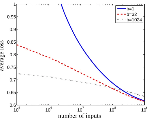
Figure 2: The effects of of the batch size when serial batching on average loss. The mini-batches algorithm was applied with different batch sizes. The x-axis presents the number of instances observed, and the y-axis presents the average loss. Note that the case b=1 is the standard serial dual-averaging algorithm.
is log2(k)ms, where k is the number of nodes in the cluster. We assumed that our search engine receives 4 queries per ms (which adds up to ten billion queries a month). Overall, the number of queries discarded between mini-batches is µ=4 log2(k).
In all of our experiments, we use the algorithmic parameter αj =L+γ√j (see Theorem 2).
We set the smoothness parameter L to a constant, and the parameterγto a constant divided by√b. This is because L depends only on the loss function f , which does not change in DMB, whileγ is proportional to σ, the standard deviation of the gradient-averages. We chose the constants by manually exploring the parameter space on a separate held-out set of 500 million queries.
We report all of our results in terms of the average loss suffered by the online algorithm. This is simply defined as(1/t)∑t
i=1f(wi,zi). We cannot plot regret, as we do not know the offline risk
minimizer w⋆.
6.1 Serial Mini-Batching
As a warm-up, we investigated the effects of modifying the mini-batch size b in a standard serial Euclidean dual averaging algorithm. This is equivalent to running the distributed simulation with a cluster size of k=1, with varying mini-batch size. We ran the experiment with b=1,2,4, . . . ,1024. Figure 2 shows the results for three representative mini-batch sizes. The experiments tell an in-teresting story, which is more refined than our theoretical upper bounds. While the asymptotic worst-case theory implies that batch-size should have no significant effect, we actually observe that mini-batching accelerates the learning process on the first 108inputs. On the other hand, after 108
105 106 107 108 109 0.5
1 1.5 2 2.5
k=1024, µ=40, b=1024
no−comm batch no−comm serial
DMB
number of inputs
av
er
ag
e
lo
ss
105 106 107 108 109
0.5 1 1.5 2 2.5
k=32, µ=20, b=1024
no−comm batch no−comm serial
DMB
number of inputs
av
er
ag
e
lo
ss
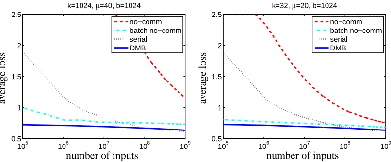
Figure 3: Comparing DBM with the serial algorithm and the no-communication distributed algo-rithm. Results for a large cluster of k=1024 machines are presented on the left. Results for a small cluster of k=32 machines are presented on the right.
for many different parameter setting, during the initial stage when we tuned the parameters on a held-out set.
Similar transient behaviors also exist for multi-step stochastic gradient methods (see, e.g., Polyak, 1987, Section 4.3.2), where the multi-step interpolation of the gradients also gives the smoothing effects as using averaged gradients. Typically such methods converge faster in the early iterations when the iterates are far from the optimal solution and the relative value of the stochastic noise is small, but become less effective asymptotically.
6.2 Evaluating DBM
Next, we compared the average loss of the DBM algorithm with the average loss of the serial algorithm and the no-communication algorithm (where each cluster node works independently). We tried two versions of the no-communication solution. The first version simply runs k independent copies of the serial prediction algorithm. The second version runs k independent copies of the serial mini-batch algorithm, with a mini-batch size of 128. We included the second version of the no-communication algorithm after observing that mini-batching has significant advantages even in the serial setting. We experimented with various cluster sizes and various mini-batch sizes. As mentioned above, we set the latency of the DBM algorithm to µ=4 log2(k). Taking a cue from our theoretical analysis, we set the batch size to b=m1/3≃1024. We repeated the experiment for
105 106 107 108 109 0.62
0.64 0.66 0.68 0.7 0.72 0.74 0.76
b=1024
µ=40
µ=320
µ=1280
µ=5120
number of inputs
av
er
ag
e
lo
ss
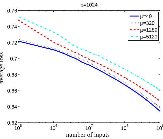
Figure 4: The effects of increased network latency. The loss of the DMB algorithm is reported with different latencies as measured by µ. In all cases, the batch size is fixed at b=1024.
6.3 The Effects of Latency
Network latency results in the DMB discarding gradients, and slows down the algorithm’s progress. The theoretical analysis shows that this waste is negligible in the asymptotic worst-case sense. How-ever, latency will obviously have some negative effect on any finite prefix of the input stream. We examined what would happen if the single-link latency were much larger than our 0.5ms estimate (e.g., if the network is very congested or if the cluster nodes are scattered across multiple datacen-ters). Concretely, we set the cluster size to k=1024 nodes, the batch size to b=1024, and the single-link latency to 0.5,1,2, . . . ,512 ms. That is, 0.5ms mimics a realistic 1Gbs Ethernet link, while 512ms mimics a network whose latency between any two machines is 1024 times greater, namely, each vector-sum operation takes a full second to complete. Note that µ is still computed as before, namely, for latency 0.5·2p, µ=2p4 log2(k) =2p·40. Figure 4 shows how the average loss curve reacts to four representative latencies. As expected, convergence rate degrades monotonically with latency. When latency is set to be 8 times greater than our realistic estimate for 1Gbs Ethernet, the effect is minor. When the latency is increased by a factor of 1024, the effect becomes more noticeable, but still quite small.
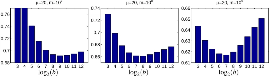
6.4 Optimal Mini-Batch Size
3 4 5 6 7 8 9 10 11 12 0.68
0.7 0.72 0.74 0.76
µ=20, m=107
log2(b)
3 4 5 6 7 8 9 10 11 12 0.66
0.68 0.7 0.72 0.74
µ=20, m=108
log2(b)
3 4 5 6 7 8 9 10 11 12 0.61
0.62 0.63 0.64 0.65 0.66
µ=20, m=109
log2(b)
Figure 5: The effect of different mini-batch sizes (b) on the DBM algorithm. The DMB algorithm was applied with different batch sizes b=8, . . . ,4096. The loss is reported after 107 instances (left), 108instances (middle) and 109instances (right).
that b=Θ(m1/3) is a pretty good concrete choice. We have already seen that larger batch sizes accelerate the initial learning phase, even in a serial setting. We set the cluster size to k=32 and set batch size to 8,16, . . . ,4096. Note that b=32 is the case where each node processes a single example before engaging in a vector-sum network operation. Figure 5 depicts the average loss after 107,108,and 109inputs. As noted in the serial case, larger batch sizes (b=512) are beneficial at first (m=107), while smaller batch sizes(b=128) are better in the end (m=109).
6.5 Discussion
We presented an empirical evaluation of the serial mini-batch algorithm and its distributed version, the DMB algorithm, on a realistic web-scale online prediction problem. As expected, the DMB algorithm outperforms the n¨aive no-communication algorithm. An interesting and somewhat unex-pected observation is the fact that the use of large batches improves performance even in the serial setting. Moreover, the optimal batch size seems to generally decrease with time.
We also demonstrated the effect of network latency on the performance of the DMB algorithm. Even for relatively large values of µ, the degradation in performance was modest. This is an encour-aging indicator of the efficiency and robustness of the DMB algorithm, even when implemented in a high-latency environment, such as a grid.
7. Related Work
In recent years there has been a growing interest in distributed online learning and distributed opti-mization.