Dynamic Affine-Invariant Shape-Appearance Handshape Features
and Classification in Sign Language Videos
Anastasios Roussos [email protected]
Queen Mary, University of London
School of Electronic Engineering and Computer Science Mile End Road, London E1 4NS, UK
Stavros Theodorakis [email protected]
Vassilis Pitsikalis [email protected]
Petros Maragos [email protected]
National Technical University of Athens School of Electrical and Computer Engineering Zografou Campus, Athens 15773, Greece
Editor:Isabelle Guyon and Vassilis Athitsos
Abstract
We propose the novel approach of dynamic affine-invariant shape-appearance model (Aff-SAM) and employ it for handshape classification and sign recognition in sign language (SL) videos. Aff-SAM offers a compact and descriptive representation of hand configurations as well as regularized model-fitting, assisting hand tracking and extracting handshape features. We construct SA images representing the hand’s shape and appearancewithout landmark points. We model the variation of the images by linear combinations of eigenimages followed by affine transformations, account-ing for 3D hand pose changes and improvaccount-ing model’s compactness. We also incorporate static and dynamic handshape priors, offering robustness in occlusions, which occur often in signing. The approach includes anaffine signer adaptationcomponent at the visual level, without requiring training from scratch a new singer-specific model. We rather employ a short development data set to adapt the models for a new signer. Experiments on the Boston-University-400 continuous SL corpus demonstrate improvements on handshape classification when compared to other feature ex-traction approaches. Supplementary evaluations of sign recognition experiments, are conducted on a multi-signer, 100-sign data set, from the Greek sign language lemmas corpus. These explore the fusion with movement cues as well as signer adaptation of Aff-SAM to multiple signers providing promising results.
Keywords: affine-invariant shape-appearance model, landmarks-free shape representation, static and dynamic priors, feature extraction, handshape classification
1. Introduction
based human-computer interaction. Nevertheless, these tasks still pose several challenges, which are mainly due to the fast movement and the great variation of the hand’s 3D shape and pose.
In this article, we propose a novel modeling of the shape and dynamics of the hands during signing that leads to efficient handshape features, employed to train statistical handshape models and finally for handshape classification and sign recognition. Based on 2D images acquired by a monocular camera, we employ a video processing approach that outputs reliable and accurate masks for the signer’s hands and head. We constructShape-Appearance (SA) imagesof the hand by combining 1) the hand’s shape, as determined by its 2D hand mask, with 2) the hand’s appearance, as determined by a normalized mapping of the colors inside the hand mask. The proposed modeling does not employ any landmark points and bypasses the point correspondence problem. In order to design a model of the variation of the SA images, which we callAffine Shape-Appearance Model
(Aff-SAM), we modify the classic linear combination of eigenimages by incorporating 2D affine transformations. These effectively account for various changes in the 3D hand pose and improve the model’s compactness. After developing a procedure for the training of the Aff-SAM, we design a robust hand tracking system by adopting regularized model fitting that exploits prior information about the handshape and its dynamics. Furthermore, we propose to use as handshape features the Aff-SAM’s eigenimage weights estimated by the fitting process.
The extracted features are fed into statistical classifiers based on Gaussian mixture models (GMM), via a supervised training scheme. The overall framework is evaluated and compared to other methods in extensive handshape classification experiments. The SL data are from the Boston University BU400 corpus (Neidle and Vogler, 2012). The experiments are based on manual an-notation of handshapes that contain 3D pose parameters and the American Sign Language (ASL) handshape configuration. Next, we define classes that account for varying dependency of the hand-shapes w.r.t. the orientation parameters. The experimental evaluation addresses first, in a qualitative analysis the feature spaces via a cluster quality index. Second, we evaluate via supervised train-ing a variety of classification tasks accounttrain-ing for dependency w.r.t. orientation/pose parameters, with/without occlusions. In all cases we also provide comparisons with other baseline approaches or more competitive ones. The experiments demonstrate improved feature quality indices as well as classification accuracies when compared with other approaches. Improvements in classification accuracy for the non-occlusion cases are on average of 35% over baseline methods and 3% over more competitive ones. Improvements by taking into account the occlusion cases are on average of 9.7% over the more competitive methods.
In addition to the above, we explore the impact of Aff-SAM features in a sign recognition task based on statistical data-driven subunits and hidden Markov models. These experiments are applied on data from the Greek Sign Language (GSL) lemmas corpus (DictaSign, 2012), for two different signers, providing a test-bed for the fusion with movement-position cues, and as evaluation of the affine-adapted SA model to a new signer, for which there has been no Aff-SAM training. These experiments show that the proposed approach can be practically applied to multiple signers without requiring training from scratch for the Aff-SAM models.
2. Background and Related Work
including the one presented here, use skin color segmentation for hand detection (Argyros and Lourakis, 2004; Yang et al., 2002; Sherrah and Gong, 2000). Some degree of robustness to illumi-nation changes can be achieved by selecting color spaces, as theHSV,YCbCror theCIE-Lab, that separate the chromaticity from the luminance components (Terrillon et al., 2000; Kakumanu et al., 2007). In our approach, we adopt theCIE-Labcolor space, due to its property of being perceptually uniform. Cui and Weng (2000) and Huang and Jeng (2001) employ motion cues assuming the hand is the only moving object on a stationary background, and that the signer is relatively still.
The next visual processing step is the hand tracking. This is usually based on blobs (Starner et al., 1998; Tanibata et al., 2002; Argyros and Lourakis, 2004), hand appearance (Huang and Jeng, 2001), or hand boundary (Chen et al., 2003; Cui and Weng, 2000). The frequent occlusions during signing make this problem quite challenging. In order to achieve robustness against occlusions and fast movements, Zieren et al. (2002), Sherrah and Gong (2000) and Buehler et al. (2009) apply probabilistic or heuristic reasoning for simultaneous assignment of labels to the possible hand/face regions. Our strategy for detecting and labeling the body-parts shares similarities with the above. Nevertheless, we have developed a more elaborate preprocessing of the skin mask, which is based on the mathematical morphology and helps us separate the masks of different body parts even in cases of overlaps.
Furthermore, a crucial issue to address in a SL recognition system is hand feature extraction, which is the focus of this paper. A commonly extracted positional feature is the 2D or 3D center-of-gravity of the hand blob (Starner et al., 1998; Bauer and Kraiss, 2001; Tanibata et al., 2002; Cui and Weng, 2000), as well as motion features (e.g., Yang et al., 2002; Chen et al., 2003). Several works use geometric measures related to the hand, such as shape moments (Hu, 1962; Starner et al., 1998) or sizes and distances between fingers, palm, and back of the hand (Bauer and Kraiss, 2001), though the latter employs color gloves. In other cases, the contour that surrounds the hand is used to extract translation, scale, and/or in-plane rotation invariant features, such as Fourier descriptors (Chen et al., 2003; Conseil et al., 2007).
Segmented hand images are usually normalized for size, in-plane orientation, and/or illumina-tion and afterwards principal component analysis (PCA) is often applied for dimensionality reduc-tion and descriptive representareduc-tion of handshape (Sweeney and Downton, 1996; Birk et al., 1997; Cui and Weng, 2000; Wu and Huang, 2000; Deng and Tsui, 2002; Dreuw et al., 2008; Du and Piater, 2010). Our model uses a similar framework but differs from these methods mainly in the following aspects. First, we employ a more general class of transforms to align the hand images, namely affine transforms that extend both similarity transforms, used, for example, by Birk et al. (1997) and translation-scale transforms as in the works of Cui and Weng (2000), Wu and Huang (2000) and Du and Piater (2010). In this way, we can effectively approximate a wider range of changes in the 3D hand pose. Second, the estimation of the optimum transforms is done simultaneously with the estimation of the PCA weights, instead of using a pipeline to make these two sets of estimations. Finally, unlike all the above methods, we incorporate combined static and dynamic priors, which make these estimations robust and allow us to adapt an existing model on a new signer.
R L H
R L H
HR L
HR L
HR L
RL H
R L H
RL H
HR L
R L H
Figure 1: Output of the initial hands and head tracking in two videos of two different signers, from different databases. Example frames with extracted skin region masks and assigned body-part labelsH(head),L(left hand),R(right hand).
way, it avoids shape representation through landmarks and the cumbersome manual annotation re-lated to that.
Other more general purpose approaches have also been seen in the literature. A method earlier employed for action-type features is the histogram of oriented gradients (HOG): these descriptors are used for the handshapes of a signer (Buehler et al., 2009; Liwicki and Everingham, 2009; Ong et al., 2012). Farhadi et al. (2007) employ the scale invariant feature transform (SIFT) descrip-tors. Finally, Thangali et al. (2011) take advantage of linguistic constraints and exploit them via a Bayesian network to improve handshape recognition accuracy. Apart from the methods that pro-cess 2D hand images, there are methods built on a 3D hand model, in order to estimate the finger joint angles and the 3D hand pose (Athitsos and Sclaroff, 2002; Fillbrandt et al., 2003; Stenger et al., 2006; Ding and Martinez, 2009; Agris et al., 2008). These methods have the advantage that they can potentially achieve view-independent tracking and feature extraction; however, their model fitting process might be computationally slow.
a∗
b
∗
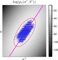
log(ps(a∗, b∗))
−120 −100 −80 −60 −40 −20
Figure 2: Skin color modeling. Training samples in thea∗-b∗ space and fitted pdfps(a∗,b∗). The ellipse bounds the colors that are classified to skin, according to the thresholding of
ps(a∗(x),b∗(x)). The straight line corresponds to the first PCA eigendirection on the skin samples and determines the projection that defines the mapping g(I) used in the Shape-Appearance images formation.
3. Visual Front-End Preprocessing
The initial step of the visual processing is not the main focus of our method, nevertheless we de-scribe it for completeness and reproducibility. The output of this subsystem at every frame is a set of skin region masks together with one or multiplelabelsassigned to every region, Figure 1. These labels correspond to thebody-parts of interestfor sign language recognition: head (H), left hand (L) and right hand (R). The case that a mask has multiple labels reflects anoverlapof the 2D regions of the corresponding body-parts, that is, there is anocclusionof some body-parts. Referring for exam-ple to the right hand, there are the following cases: 1) The system outputs a mask that contains the right hand only, therefore there isno occlusionrelated to that hand, and 2) The output mask includes the right hand as well as other body-part region(s), therefore there is anocclusion. As presented in Section 4, the framework of SA refines this tracking while extracting handshape features.
3.1 Probabilistic Skin Color Modeling
We are based on the color cue for body-parts detection. We consider a Gaussian model of the signer’s skin color in the perceptually uniform color space CIE-Lab, after keeping the two chro-maticity components a∗, b∗, to obtain robustness to illumination (Cai and Goshtasby, 1999). We assume that the (a∗,b∗) values of skin pixels follow a bivariate Gaussian distribution ps(a∗,b∗), which is fitted using a training set of color samples (Figure 2). These samples are automatically extracted from pixels of the signer’s face, detected using a face detector (Viola and Jones, 2003).
3.2 Morphological Processing of Skin Masks
In each frame, a first estimation of the skin maskS0is derived by thresholding at every pixelxthe
valueps(a∗(x),b∗(x))of the learned skin color distribution, see Figures 2, 3(b). The corresponding threshold is determined so that a percentage of the training skin color samples are classified to skin. This percentage is set to 99% to cope with training samples outliers. The skin maskS0may contain
spurious regions or holes inside the head area due to parts with different color, as for instance eyes, mouth. For this, we regularizeS0with tools from mathematical morphology (Soille, 2004; Maragos,
(a) Input (b)S0 (c)S2 (d)S2⊖Bc (e) SegmentedS2
Figure 3: Results of skin mask extraction and morphological segmentation. (a) Input. (b) Initial skin mask estimationS0. (c) Final skin maskS2(morphological refinement). (d) Erosion S2⊖Bc of S2 and separation of overlapped regions. (e) Segmentation of S2 based on
competitive reconstruction opening.
components, not connected to the border of the image. In order to fill also some background regions that are not holes in the strict sense but are connected to the image border passing from a small “canal”, we designed a filter that we callgeneralized hole filling. This filter yields a refined skin mask estimationS1=S0∪
H
(S0)∪
H
(S0•B)⊕B whereBis a structuring element with size 5×5pixels, and⊕and•denotes Minkowski dilation, closing respectively. The connected components (CCs) of relevant skin regions can be at most three (corresponding to the head and the two hands) and cannot have an area smaller than a thresholdAmin, which corresponds to the smallest possible area of a hand region for the current signer and video acquisition conditions. Therefore, we apply an
area openingwith a varying threshold value: we find all CCs ofS1, compute their areas and finally
discard all the components whose area is not on the top 3 or is less thanAmin. This yields the final skin maskS2, see Figure 3(c).
3.3 Morphological Segmentation of the Skin Masks
In the frames whereS2contains three CCs, these yield an adequate segmentation. On the contrary,
whenS2contains less than three CCs, the skin regions of interest occlude each other. In such cases
though, the occlusions are not always essential: different skin regions inS2may be connected via a
thin connection, Figure 3(c). Therefore we further segment the skin masks of some frames by sep-arating occluded skin regions with thin connections: IfS2containsNcc<3 connected components, we find the CCs ofS2⊖Bc, Figure 3(d), for a structuring elementBc of small radius, for example, 3 pixels and discard those CCs whose area is smaller thanAmin. A number of remaining CCs not greater thanNccimplies the absence of any thin connection, thus does not provide any occlusion separation. Otherwise, we use each one of these CCs as the seed of a different segment and expand it to coverS2. For this we propose acompetitive reconstruction opening, see Figure 3(e), described
by the following iterative algorithm: In every iteration 1) each evolving segment expands using its conditional dilation by the 3×3 cross, relative toS2, 2) pixels belonging to more than one segment
are excluded from all segments. This means that segments are expanded insideS2but their
expan-sion stops wherever they meet other segments. The above two steps are repeated until all segments remain unchanged.
3.4 Body-part Label Assignment
Note that these ellipses yield a rough estimate of the shapes of the occluded regions and contribute to the correct assignment of labels after each occlusion. A detailed presentation of this algorithm falls beyond the scope of this article. A brief description follows. Non-occlusions: For the hands’ labels, given their values in the previous frames, we employ a prediction of the centroid position of each hand region taking into account three preceding frames and using a constant acceleration model. Then, we assign the labels based on minimum distances between the predicted positions and the segments’ centroids. We also fit one ellipse on each segment since an ellipse can coarsely approximate the hand or head contour. Occlusions: Using the parameters of the body-part ellipses already computed from the three preceding frames, we employ similarly forward prediction for all ellipses parameters, assuming constant acceleration. We face non-disambiguated cases by obtaining an auxiliary centroid estimation of each body-part via template matching of the corresponding image region between consecutive frames. Then, we repeat the estimations backwards in time. Forward and backward predictions, are fused yielding a final estimation of the ellipses’ parameters for the signer’s head and hands. Figure 1 depicts the output of the initial tracking in sequences of frames with non-occlusion and occlusion cases. We observe that the system yields accurate skin extraction and labels assignment.
4. Affine Shape-Appearance Modeling
In this section, we describe the proposed framework of dynamic affine-invariant shape-appearance model which offers a descriptive representation of the hand configurations as well as a simultaneous hand tracking and feature extraction process.
4.1 Representation by Shape-Appearance images
We aim to model all possible configurations of the dominant hand during signing, using directly the 2D hand images. These images exhibit a high diversity due to the variations on the configuration and 3D hand pose. Further, the set of the visible points of the hand is significantly varying. Therefore, it is more effective to represent the 2D handshape without using any landmarks. We thus represent the handshape by implicitly using its binary maskM, while incorporating also theappearanceof the hand, that is, the color values inside this mask. These values depend on the hand texture and shading, and offer crucial 3D information.
IfI(x) is a cropped part of the current color frame around the hand maskM, then the hand is represented by the followingShape-Appearance (SA) image(see Figure 4):
f(x) =
(
g(I(x)), if x∈M
−cb, otherwise
,
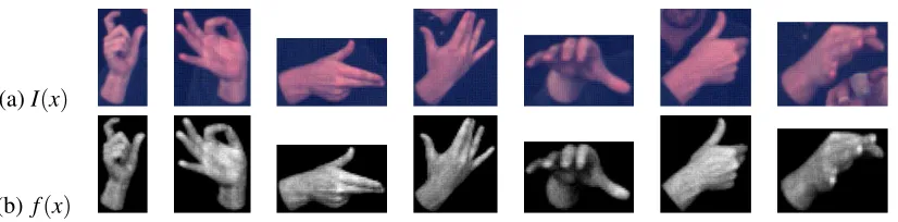
(a)I(x)
(b) f(x)
Figure 4: Construction of Shape-Appearance images. (a) Cropped hand images I(x). (b) Corre-sponding Shape-Appearance images f(x). For the foreground of f(x) we use the most descriptive feature of the skin chromaticity. The background has been replaced by a con-stant value that is out of the range of the foreground values.
The mappingg(I)is constructed as follows. First we transform each color valueIto theCIE-Lab
color space, then keep only the chromaticity componentsa∗,b∗. Finally, we output the normalized weight of the first principal eigendirection of the PCA on the skin samples, that is the major axis of the Gaussian ps(a∗,b∗), see Section 3.1 and Figure 2(c). The outputg(I)is the most descriptive value for the skin pixels’ chromaticity. Furthermore, if considered together with the training of
ps(a∗,b∗), the mappingg(I)is invariant to global similarity transforms of the values (a∗,b∗). There-fore, the SA images are invariant not only to changes of the luminance componentLbut also to a wide set of global transforms of the chromaticity pair (a∗,b∗). As it will be described in Section 5, this facilitates the signer adaptation.
4.2 Modeling the Variation of Hand Shape-Appearance Images
Following Matthews and Baker (2004), the SA images of the hand, f(x), are modeled by a linear combination of predefined variation images followed by an affine transformation:
f(Wp(x))≈A0(x) +
Nc
∑
i=1
λiAi(x),x∈ΩM. (1)
A0(x) is the mean image, Ai(x) areNc eigenimages that model the linear variation. These images can be considered as affine-transformation-free images. In addition,λ= (λ1· · ·λNc)are the weights of the linear combination andWpis an affine transformation with parameters p= (p1· · ·p6)that is
defined as follows:
Wp(x,y) =
1+p1 p3 p5 p2 1+p4 p6
x y
1
.
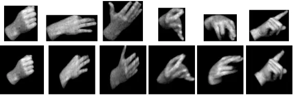
Figure 5: Semi-automatic affine alignment of a training set of Shape-Appearance images. (Top row) 6 out of 500 SA images of the training set. (Bottom row) Corresponding transformed images, after affine alignment of the training set. A video that demonstrates this affine alignment is available online (see text).
We will hereafter refer to the proposed model asShape-Appearance Model (SAM). A specific model of hand SA images is defined from the base imageA0(x)and the eigenimagesAi(x), which are statistically learned from training data. The vectorspandλare the model parameters that fit the
model to the hand SA image of every frame. These parameters are considered as features of hand pose and shape respectively.
4.3 Training of the SAM Linear Combination
In order to train the hand SA images model, we employ a representative set of handshape images from frames where the modeled hand is fully visible and non-occluded. Currently, this set is con-structed by a random selection of approximately 500 such images. To exclude the variation that can be explained by the affine transformations of the model, we apply a semi-automatic affine alignment of the training SA images. For this, we use the framework ofprocrustes analysis(Cootes and Tay-lor, 2004; Dryden and Mardia, 1998), which is an iterative process that is repeatedly applying 1-1 alignments between pairs of training samples. In our case, the 1-1 alignments are affine alignments, implemented by applying the inverse-compositional (IC) algorithm (Gross et al., 2005) on pairs of SA images.
The IC algorithm result depends on the initialization of the affine warp, since the algorithm converges to a local optimum. Therefore, in each 1-1 alignment we test two different initializa-tions: Using the binary masksMof foreground pixels of the two SA images, these initializations correspond to the two similarity transforms that make the two masks have the same centroid, area and orientation.1 Among the two alignment results, the plausible one is kept, according to manual feedback from a user.
It must be stressed that the manual annotation of plausible alignment results is needed only dur-ing the traindur-ing of the SA model, not durdur-ing the fittdur-ing of the model. Also, compared to methods that use landmarks to model the shape (e.g., Cootes and Taylor, 2004; Matthews and Baker, 2004; Ahmad et al., 1997; Bowden and Sarhadi, 2002), the amount of manual annotation during training is substantially decreased: The user here is not required to annotate points but just make a binary de-cision by choosing the plausible result of 1-1 alignments. Other related methods for aligning sets of images are described by Learned-Miller (2005) and Peng et al. (2010). However, the adopted
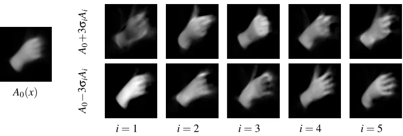
A0(x)
A0
+
3
σi
Ai
A0
−
3
σi
Ai
i=1 i=2 i=3 i=4 i=5
Figure 6: Result of the PCA-based learning of the linear variation images of Equation (1): Mean imageA0(x) and principal modes of variation that demonstrate the first 5 eigenimages.
The top (bottom) row corresponds to deviating from A0 in the direction of the
corre-sponding eigenimage, with a weight of 3σi(-3σi), whereσiis the standard deviation of the corresponding component.
crustes analysis framework facilitates the incorporation of the manual annotation in the alignment procedure. Figure 5 shows some results from the affine alignment of the training set. For more details, please refer to the following URL that contains a video demonstration of the training set alignment:http://cvsp.cs.ntua.gr/research/sign/aff_SAM. We observe that the alignment produces satisfactory results, despite the large variability of the images of the training set. Note that the resolution of the aligned images is 127×133 pixels.
Then, the imagesAi of the linear combination of the SA model are statistically learned using principal component analysis (PCA) on the aligned training SA images. The numberNcof eigenim-ages kept is a basic parameter of the SA model. Using a largerNc, the model can better discriminate different hand configurations. On the other hand, ifNc gets too large, the model may not general-ize well, in the sense that it will be consumed on explaining variation due to noise or indifferent information. In the setup of our experiments, we have practically concluded that the valueNc=35 is quite effective. With this choice, the eigenimages kept explain 78% of the total variance of the aligned images.
Figure 6 demonstrates results of the application of PCA. Even though the modes of principal variation do not correspond to real handshapes, there is some intuition behind the influence of each eigenimage at the modeled hand SA image. For example, the first eigenimageA1has mainly to do
with the foreground appearance: as its weight gets larger, the foreground intensities get darker and vice-versa. As another example, we see that by increasing the weight of the second eigenimageA2,
the thumb is extended. Note also that when we decrease the weight ofA4all fingers extend and start
detaching from each other.
4.4 Regularized SAM Fitting with Static and Dynamic Priors
occlusions, we exploit prior information about the handshape and its dynamics. Therefore, we minimize the following energy:
E(λ,p) =Erec(λ,p) +wSES(λ,p) +wDED(λ,p), (2)
whereErecis a reconstruction error term. The termsES(λ,p)andED(λ,p)correspond to static and dynamic priors on the SAM parametersλandp. The valueswS,wDare positive weights that control the balance between the 3 terms.
The reconstruction error term Erecis a mean square difference defined by:
Erec(λ,p) = 1
NM
∑
x
A0(x) +
Nc
∑
i=1
λiAi(x)−f(Wp(x))
2
,
where the above summation is done over all theNM pixelsxof the domain of the imagesAi(x).
The static priors term ES(λ,p)ensures that the solution stays relatively close to the parameters mean valuesλ0,p0:
ES(λ,p) = 1
Nc
kλ−λ0k2Σλ+
1
Np
kp−p0k2Σp ,
where Nc andNp are the dimensions of λ and p respectively (since we model affine transforms,
Np=6). These numbers act as normalization constants, since they correspond to the expected values of the quadratic terms that they divide. Also,ΣλandΣpare the covariance matrices ofλandp re-spectively,2which are estimated during the training of the priors (Section 4.4.2). We denote bykykA, withAbeing aN×N symmetric positive-definite matrix andy∈RN, the following Mahalanobis distance fromyto 0:
kykA,pyTA−1y.
Using such a distance, the term ES(λ,p) penalizes the deviation from the mean values but in a weighted way, according to the appropriate covariance matrices.
The dynamic priors term ED(λ,p)makes the solution stay close to the parameters estimations
λe=λe[n],pe=pe[n]based on already fitted values on adjacent frames (for how these estimations are derived, see Section 4.4.1):
ED(λ,p) = 1
Nc
kλ−λek2Σελ+ 1
Np
kp−pek2Σεp , (3) where Σελ andΣεp are the covariance matrices of the estimation errors of λ and p respectively, see Section 4.4.2 for the training of these quantities too. The numbers Nc and Np act again as normalization constants. Similarly toES(λ,p), the termED(λ,p) penalizes the deviation from the predicted values in a weighted way, by taking into account the corresponding covariance matrices. Since the parametersλare the weights of the eigenimagesAi(x)derived from PCA, we assume that their meanλ0=0 and their covariance matrixΣλis diagonal, which means that each component of
λis independent from all the rest.
It is worth mentioning that the energy-balancing weightswS,wDare not constant through time, but depend on whether the modeled hand in the current frame is occluded or not (this information is provided by the initial tracking preprocessing step of Section 3). In the occlusion cases, we are
less confident than in the non-occlusion cases about the input SA image f(x), which is involved in the termErec(λ,p). Therefore, in these cases we obtain more robustness by increasing the weights
wS,wD. In parallel, we decrease the relative weight of the dynamic priors term wSwD+wD, in order to prevent error accumulation that could be propagated in long occlusions via the predictionsλe, pe. After parameters tuning, we have concluded that the following choices are effective for the setting of our experiments: 1)wS=0.07,wD=0.07 for the non-occluded cases and 2)wS=0.98,wD=0.42 for the occluded cases.
An input video is split into much smaller temporal segments, so that the SAM fitting is sequen-tialinside every segment as wellindependentfrom the fittings in all the rest segments: All the video segments of consecutive non-occluded and occluded frames are found and the middle frame of each segment is specified. For each non-occluded segment, we start from its middle frame and we get 1) a segment with forward direction by ending to the middle frame of the next occluded segment and 2) a segment with backward direction by ending after the middle frame of the previous occluded segment. With this splitting, we increase the confidence of the beginning of each sequential fit-ting, since in a non-occluded frame the fitting can be accurate even without dynamic priors. In the same time, we also get the most out of the dynamic priors, which are mainly useful in the occluded frames. Finally, this splitting strategy allows a high degree of parallelization.
4.4.1 DYNAMICALMODELS FOR PARAMETERPREDICTION
In order to extract the parameter estimations λe, pe that are used in the dynamic prior term ED (3), we use linear prediction models (Rabiner and Schafer, 2007). At each frame n, a varying numberK=K(n)of already fitted frames is used for the parameter prediction. If the frame is far enough from the beginning of the current sequential fitting,Ktakes its maximum value,Kmax. This maximum length of a prediction window is a parameter of our system (in our experiments, we used
Kmax=8 frames). If on the other hand, the frame is close to the beginning of the corresponding segment, thenKvaries from 0 toKmax, depending on the number of frames of the segment that have been already fitted.
IfK=0, we are at the starting frame of the sequential fitting, therefore no prediction from other available frames can be made. In this case, which is degenerate for the linear prediction, we consider that the estimations are derived from the prior means λe =λ0, pe = p0 and also that Σελ =Σε,
Σεp=Σp, which results toED(λ,p) =ES(λ,p). In all the rest cases, we apply the framework that is described next.
Given the prediction window valueK, the parameters λare predicted using the following au-toregressive model:
λe[n] = K
∑
ν=1
Aνλ[n∓ν],
where the−sign (+sign) corresponds to the case of forward (backward) prediction. Also, Aνare
As far as the parameters pare concerned, they do not have zero mean and we cannot consider them as independent since, in contrast toλ, they are not derived from a PCA. Therefore, in order to apply the same framework as above, we consider the following re-parametrization:
ep=UpT(p−p0)⇔p=p0+Upep,
where the matrixUpcontains column-wise the eigenvectors ofΣp. The new parametersephave zero mean and diagonal covariance matrix. Similarly toλ, the normalized parametersep are predicted using the following model:
epe[n] =
K
∑
ν=1
Bνep[n∓ν],
where Bνare the corresponding weight matrices which again are all considered diagonal.
4.4.2 AUTOMATICTRAINING OF THESTATIC ANDDYNAMICPRIORS
In order to apply the regularized SAM fitting, we first learn the priors on the parameters λand p
and their dynamics. This is done by training subsequences of frames where the modeled hand is not occluded. This training does not require any manual annotation. We first apply a random selection of such subsequences from videos of the same signer. Currently, the randomly selected subsequences used in the experiments are 120 containing totally 2882 non-occluded frames and coming from 3 videos. In all the training subsequences, we fit the SAM in each frame independently by minimizing the energy in Equation (2) withwS=wD=0 (that is without prior terms). In this way, we extract fitted parametersλ,pfor all the training frames. These are used to train the static and dynamic priors.
4.4.3 STATICPRIORS
In this case, for both cases of λand p, the extracted parameters from all the frames are used as samples of the same multivariate distribution, without any consideration of their successiveness in the training subsequences. In this way, we form the training setsTλandTpthat correspond toλand
prespectively. Concerning the parameter vectorλ, we have assumed that its meanλ0=0 and its covariance matrixΣλis diagonal. Therefore, only the diagonal elements ofΣλ, that is the variances
σ2
λi of the components ofλ, are to be specified. This could be done using the result of the PCA (Section 4.2), but we employ the training parameters ofTλthat come from the direct SAM fitting, since they are derived from a process that is closer to the regularized SAM fitting. Therefore, we estimate eachσ2
λi from the empirical variance of the corresponding componentλiin the training set
Tλ. Concerning the parameters p, we estimate p0andΣpfrom the empirical mean and covariance matrix of the training setTp.
4.4.4 DYNAMICPRIORS
As already mentioned, for each prediction direction (forward, backward) and for each lengthKof the prediction window, we consider a different prediction model. The(K+1)-plets3of samples for each one of these models are derived by sliding the appropriate window in the training sequences. In order to have as good accuracy as possible, we do not make any zero (or other) padding in unknown parameter values. Therefore, the samples are picked only when the window fits entirely inside the
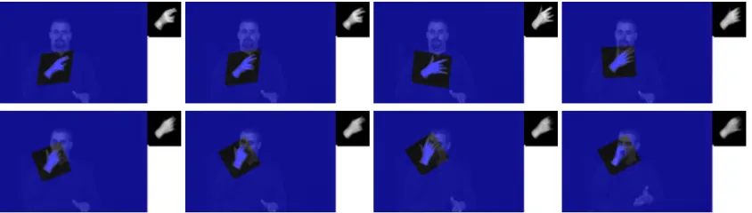
Figure 7: Regularized Shape-Appearance Model fitting in a sign language video. In every input frame, we superimpose the model-based reconstruction of the hand in the frame domain,
A0(Wp−1(x)) +∑ λiAi(Wp−1(x)). In the upper-right corner, we display the reconstruction in the model domain,A0(x) +∑ λiAi(x), which determines the optimum weights λ. A demo video is available online (see text).
training sequence. Similarly to linear predictive analysis (Rabiner and Schafer, 2007) and other tracking methods that use dynamics (e.g., Blake and Isard, 1998) we learn the weight matrices Aν, Bν by minimizing the mean square estimation error over all the prediction-testing frames. Since we have assumed that Aν and Bν are diagonal, this optimization is done independently for each component ofλandep, which is treated as 1D signal. The predictive weights for each component are thus derived from the solution of an ordinary least squares problem. The optimum values of the mean squared errors yield the diagonal elements of the prediction errors’ covariance matricesΣελ andΣεep, which are diagonal.
4.4.5 IMPLEMENTATION ANDRESULTS OFSAM FITTING
The energyE(λ,p)(2) of the proposed regularized SAM fitting is a special case of the general ob-jective function that is minimized by the simultaneous inverse compositional with a prior (SICP) algorithm of Baker et al. (2004). Therefore, in order to minimizeE(λ,p), we specialize this algo-rithm for the specific types of our prior terms. Details are given in the Appendix A. At each frame
nof a video segment, the fitting algorithm is initialized as follows. If the current frame is not the starting frame of the sequential fitting (that isK(n)6=0), then the parameters λ, pare initialized from the predictions λe, pe. Otherwise, if K(n) =0, we test as initializations the two similarity transforms that, when applied to the SAM mean imageA0, make its mask have the same centroid,
area and orientation as the mask of the current frame’s SA image. We twice apply the SICP al-gorithm using these two initializations, and finally choose the initialization that yields the smallest regularized energyE(λ,p).
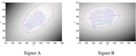
non-Signer A Signer B
Figure 8: Skin color modeling for the two signers of the GSL lemmas corpus, where we test the signer adaptation. Training samples in the a∗-b∗ chromaticity space and fitted pdf’s
ps(a∗,b∗). In each case, the straight line defines the normalized mapping g(I) used in the Shape-Appearance images formation.
occlusion cases, since the prior terms keep the result closer to the SAM mean imageA0. In addition,
extensive handshape classification experiments were performed in order to evaluate the extracted handshape features employing the proposed Aff-SAM method (see Section 7).
5. Signer Adaptation
We develop a method for adapting a trained Aff-SAM model to a new signer. This adaptation is facilitated by the characteristics of the Aff-SAM framework. Let us consider an Aff-SAM model trained to a signer, using the procedure described in Section 4.3. We aim to reliably adapt and fit the existing Aff-SAM model on videos from anew signer.
5.1 Skin Color and Normalization
The employed skin color modeling adapts on the characteristics of the skin color of a new signer. Figure 8 illustrates the skin color modeling for the two signers of the GSL lemmas corpus, where we test the adaptation. For each new signer, the color model is built from skin samples of a face tracker (Section 3.1, Section 4.1). Even though there is an intersection, the domain of colors classified as skin is different between the two. In addition, the mapping g(I) of skin color values, used to create the SA images, is normalized according to the skin color distribution of each signer. The differences in the lines of projection reveal that the normalized mappingg(I)is different in these two cases. This skin color adaptation makes the body-parts label extraction of the visual front-end preprocessing to behave robustly over different signers. In addition, the extracted SA images have the same range of values and are directly comparable across signers.
5.2 Hand Shape and Affine Transforms
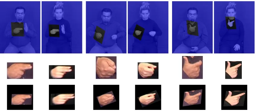
Figure 9: Alignment of the hands of two different signers, using affine transformations. First row: Input frames with superimposed rectangles that visualize the affine transformations. Sec-ond row: Cropped images around the hand.Third row: Alignment of the cropped images in a common model domain, using the affine transformations.
the affine transforms have the ability to stretch or shrink the hand images over the major hand axis. They thus automatically compensate for the fact that the second signer has thinner hands and longer fingers. In general, the class of affine transforms can effectively approximate the transformation needed to align the 2D hand shapes of different signers.
5.3 New Signer Fitting
To process a new signer the visual front-end is applied as in Section 3. Then, we only need to re-train the static and dynamic priors on the new signer. For this, we randomly select frames where the hand is not occluded. Then, for the purposes of this training, the existing SAM is fitted on them by minimizing the energy in Equation (2) withwS=wD=0, namely the reconstruction error term without prior terms. Since the SAM is trained on another signer, this fitting is not always successful, at this step. At that point, the user annotates the frames where this fitting has succeeded. This feedback is binary and is only needed during training and for a relatively small number of frames. For example, in the case of the GSL lemmas corpus, we sampled frames from approximately 1.2% of all corpus videos of this signer. In 15% of the sampled frames, this fitting with no priors was annotated as successful. Using the samples from these frames, we learn the static and dynamic priors ofλandp, as described in Section 4.4.2 for the new signer. The regularized SAM fitting is implemented as in Section 4.4.5.
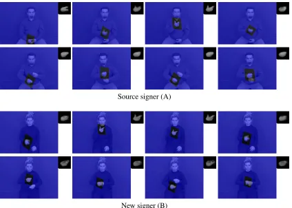
Figure 10 demonstrates results of the SAM fitting, in the case of signer adaptation. The SAM eigenimages are learned using solely Signer A. The SAM is then fitted on the signer B, as above. For comparison, we also visualize the result of the SAM fitting to the signer A, for the same sign. Demo videos for these fittings also are included in the following URL:http://cvsp.cs.ntua.gr/
Source signer (A)
New signer (B)
Figure 10: Regularized Shape-Appearance Model fitting on 2 signers. The SA model was trained on Signer A and adapted for Signer B. Demo videos are available online (see text).
the performance of the SAM fitting is satisfactory after the adaptation. In both signers, the fitting yields accurate shape estimation in non-occlusion cases.
6. Data Set and Handshape Annotation for Handshape Classification
TheSL Corpus BU400(Neidle and Vogler, 2012) is a continuous American sign language database. The background is uniform and the images have a resolution of 648x484 pixels, recorded at 60 frames per second. In the classification experiments we employ the front camera video, data from a single signer, and the story ‘Accident’. We next describe the annotation parameters required to produce the ground-truth labels. These concern the pose and handshape configurations and are essential for the supervised classification experiments.
6.1 Handshape Parameters and Annotation
(a) Front (F) (b) Side (S) (c) Bird’s (B) (d) Palm (P)
Figure 11: 3D Hand Orientation parameters: (a-c) Extended Finger Direction Parameters: (a) Signer’s front view (F), (b) Side view (S), (c) Birds’ view (B); (d) Palm orienta-tion (P). Note that we have modified the corresponding figures of Hanke (2004) with numerical parameters.
by the HamNoSys description (Hanke, 2004). The adopted annotation parameters are as follows: 1)Handshape identity (HSId)which defines the handshape configuration, that is, (‘A’, ‘B’, ‘1’, ‘C’ etc.), see Table 1 for examples. 2)3D Hand Orientation (hand pose) consisting of the following parameters (see Figure 11): i)Extended Finger Directionparameters that define the orientation of the hand axis. These correspond to the hand orientation relatively to the three planes that are de-fined relatively to: the Signer’s Front view (referred to as F), the Bird’s view (B) and the Side view (S). ii) Palm Orientationparameter (referred to as P) for a given extended finger direction. This parameter is defined w.r.t. the bird’s view, as shown in Figure 11(d).
6.2 Data Selection and Classes
We select and annotate a set of occluded and non-occluded handshapes so that 1) they cover sub-stantial handshape and pose variation as they are observed in the data and 2) they are quite frequent. More specifically we have employed three different data sets (DS): 1) DS-1: 1430 non-occluded handshape instances with 18 different HSIds. 2)DS-1-extend: 3000 non-occluded handshape in-stances with 24 different HSIds. 3)DS-2: 4962 occluded and non-occluded handshape instances with 42 different HSIds. Table 1 presents an indicative list of annotated handshape configurations and 3D hand orientation parameters.
7. Handshape Classification Experiments
HSId 1 1 4 4 5C 5 5 5 A A BL BL BL BL
3
D
h
an
d
p
o
se F 8 1 7 6 1 7 8 1 8 8 8 7 8 8
S 0 0 0 3 1 0 2 2 0 2 0 0 0 0
B 0 0 0 6 4 0 1 1 0 6 0 0 0 0
P 1 8 3 1 3 3 1 5 3 2 2 3 3 4
# insts. 14 24 10 12 27 38 14 19 14 31 10 15 23 30
exmpls.
HSId BL CUL F F U UL V Y b1 c5 c5 cS cS fO2
3
D
h
an
d
p
o
se F 8 7 7 1 7 7 8 8 7 8 8 7 8 8
S 2 0 0 2 0 0 0 0 0 0 0 0 2 0
B 6 0 0 1 0 0 0 0 0 0 6 6 6 0
P 4 3 3 3 2 3 2 2 3 3 1 3 3 1
# insts. 20 13 23 13 10 60 16 16 10 17 18 10 34 12
exmpls.
Table 1: Samples of annotated handshape identities (HSId) and corresponding 3D hand orientation (pose) parameters for the D-HFSBP class dependency and the corresponding experiment; in this case each model is fully dependent on all of the orientation parameters. ‘# insts.’ corresponds to the number of instances in the dataset. In each case, we show an example handshape image that is randomly selected among the corresponding handshape instances of the same class.
7.1 Experimental Protocol and Other Approaches
The experiments are conducted by employing cross-validation by selecting five different random partitions of the dataset into train-test sets. We employ 60% of the data for training and 40% for testing. This partitioning samples data, among all realizations per handshape class in order to equalize class occurrence. The number of realizations per handshape class are on average 50, with a minimum and maximum number of realizations in the range of 10 to 300 depending on the ex-periment and the handshape class definition. We assign to each exex-periment’s training set one GMM per handshape class; each has one mixture and diagonal covariance matrix. The GMMs are uni-formly initialized and are afterwards trained employing Baum-Welch re-estimation (Young et al., 1999). Note that we are not employing other classifiers since we are interested in the evaluation of the handshape features and not the classifier. Moreover this framework fits with common hid-den Markov model (HMM)-based SL recognition frameworks (Vogler and Metaxas, 1999), as in Section 8.
7.1.1 EXPERIMENTALPARAMETERS
Class Annotation Parameters
Dependency label HSId(H) Front(F) Side(S) Bird’s(B) Palm(P)
D-HFSBP D D D D D
D-HSBP D * D D D
D-HBP D * * D D
D-HP D * * * D
D-H D * * * *
Table 2: Class dependency on orientation parameters. One row for each model dependency w.r.t. the annotation parameters. The dependency or non-dependency state to a particu-lar parameter for the handshape trained models is noted as ‘D’ or ‘*’ respectively. For instance the D-HBP model is dependent on the HSId and Bird’s view and Palm orientation parameters.
Data Set (DS): We have experimented employing three different data sets DS-1, DS-1-extend and DS-2 (Section 6.2 for details).
Class dependency (CD):The class dependency defines the orientation parameters in which our trained models are dependent to (Table 2). Take for instance the orientation parameter ‘Front’ (F). There are two choices, either 1) construct handshape models independent to this parameter or 2) construct different handshape models for each value of the parameter. In other words, at one extent CD restricts the models generalization by making each handshape model specific to the annotation parameters, thus highly discriminable, see for instance in Table 2 the experiment corresponding to D-HFSBP. At the other extent CD extends the handshape models generalization w.r.t. to the annotation parameters, by letting the handshape models account for pose variability (that is depend only on the HSId; same HSId’s with different pose parameters are tied), see for instance experiment corresponding to the case D-H (Table 2). The CD field takes the values shown in Table 2.
7.1.2 FEATUREEXTRACTIONMETHOD
Apart from the proposed Aff-SAM method, the methods employed for handshape feature extraction are the following:
Direct Similarity Shape-Appearance Modeling (DS-SAM): Main differences of this method with Aff-SAM are as follows: 1)we replace the affine transformations that are incorporated in the SA model (1) by simplersimilaritytransforms and2)we replace the regularized model fitting by direct estimation (withoutoptimization) of the similarity transform parameters using the centroid, area and major axis orientation of the hand region followed by projection into the PCA subspace to find the eigenimage weights. Note that in the occlusion cases, this simplified fitting is done directly on the SA image of the region that contains the modeled hand as well as the other occluded body-part(s) (that is the other hand and/or the head), without using any static or dynamic priors as those of Section 4.4. This approach is similar to Birk et al. (1997) and is adapted to fit our framework.
(a)
Figure 12: Feature space for the Aff-SAM features and the D-HFSBP experiment case (see text). The trained models are visualized via projections on theλ1−λ2 plane that is formed from the weights of the two principal Aff-SAM eigenimages. Cropped handshape im-ages are placed at the models’ centroids.
using the square that tightly surrounds the hand mask, followed again by projection into the PCA subspace to find the eigenimage weights. In this simplified version too, the hand occlusion cases are treated by simply fitting the model to the Shape-Appearance image that contains the occlusion, without static or dynamic priors. This approach is similar to Cui and Weng (2000), Wu and Huang (2000) and Du and Piater (2010) and is adapted so as to fit our proposed framework.
com-−0.5 0 0.5 1 1.5
Aff−SAM
DTS−SAM DS−SAM
FD
RB M
log(DBi)
D−HFSBP D−HSBP D−HSB D−HB D−H
Figure 13: Davies-Bouldin index (DBi) in logarithmic scale (y-axis) for multiple feature spaces and varying models class dependency to the orientation parameters. Lower values of DBi indicate better compactness and separability of classes.
pactness and minor and major axis lengths of the hand region (Agris et al., 2008). Compared to the proposed Aff-SAM features we consider the rest five sets of features belonging to eitherbaseline features or more advanced features. First, the baseline features contain the FD, M and RB ap-proaches. Second, the more advanced features contain the DS-SAM and DTS-SAM methods which we have implemented as simplified versions of the proposed Aff-SAM. As it will be revealed by the evaluations, the more advanced features are more competitive than the baseline features and the comparisons with them are more challenging.
7.2 Feature Space Evaluation Results
Herein we evaluate the feature space of the Aff-SAM method. In order to approximately visualize it, we employ the weightsλ1,λ2of the two principal eigenimages of Aff-SAM. Figure 12(a) provides a visualization of the trained models per class, for the experiment corresponding to D-HFSBP class dependency (that is each class is fully dependent on orientation parameters). It presents a single indicative cropped handshape image per class to add intuition on the presentation: these images correspond to the points in the feature space that are closest to the specific classes’ centroids. We observe that similar handshape models share close positions in the space. The presented feature space is indicative and it seems clear when compared to feature spaces of other methods. To support this we compare the feature spaces with the Davies-Boulding index (DBi), which quantifies their quality. In brief, the DBi is the average over alln clusters, of the ratio of intra-cluster distances
σi versus the inter-cluster distance di,j of i,j clusters, as a measure of their separation: DBi=
1
n∑ n
i=1maxi6=j( σi+σj
Data Set # HSIds CD Occ. Feat. Method Avg.Acc.% Std.
DS-1 18 Table. 2
Aff-SAM 93.7 1.5
✗ DS-SAM 93.4 1.6
DTS-SAM 89.2 1.9
DS-1-extend 24 ‘D-H’
Aff-SAM 77.2 1.6
✗ DS-SAM 74 2.3
DTS-SAM 67 1.4
DS-2 42 Table. 2
Aff-SAM 74.9 0.9
X DS-SAM 66.1 1.1
DTS-SAM 62.7 1.4
Table 3: Experiments overview with selected average overall results over different main feature extraction methods and experimental cases of DS and CD experiments, with occlusion or not (see Section 7.1). CD: class dependency. Occ.: indicates whether the dataset includes occlusion cases. # HSIds: the number of HSId employed, Avg.Acc.: average classification accuracy, Std.: standard deviation of the classification accuracy.
indices are for varying CD field, that is the orientation parameters on which the handshape models are dependent or not (as discussed in Section 7.1) and are referred in Table 2. We observe that the DBi’s for the Aff-SAM features are lower that is the classes are more compact and more separable, compared to the other cases. The closest DBi’s are these of DS-SAM. In addition, the proposed features show stable performance over experiments w.r.t. class-dependency, indicating robustness to some amount of pose variation.
7.3 Results of Classification Experiments
We next show average classification accuracy results after 5-fold cross-validation for each experi-ment. together with the standard deviation of the accuracies. The experiments consist of 1) Class dependency and Feature variation for non-occlusion cases and 2) Class dependency and Feature variation for both occlusion and non-occlusion cases. Table 3 presents averages as well as compar-isons with other features for the three main experimental data sets discussed. The averages are over all cross-validation cases, and over the multiple experiments w.r.t. class dependency, where appli-cable. For instance, in the first block for the case ‘DS-1’, that is non-occluded data from the dataset DS-1, the average is taken over all cases of class dependency experiments as described in Table 2. For the ‘DS-1-extend’ case, the average is taken over the D-H class dependency experiment, since we want to increase the variability within each class.
7.3.1 FEATURECOMPARISONS FORNON-OCCLUDEDCASES
Next, follow comparisons by employing the referred feature extraction approaches, for two cases of data sets, while accounting for non-occluded cases.
7.3.2 DATASETDS-1
D−HFBSP D−HBSP D−HBP D−HP D−H 30
40 50 60 70 80 90 100
Class Dependency
Classification Accuracy
FD RB M DTS−SAM DS−SAM Aff−SAM
Figure 14: Classification experiments for non-occlusion cases, dataset DS-1. Classification Ac-curacy for varying experiments (x-axis) that is the dependency of each class w.r.t. the annotation parameters [H,F,B,S,P] and the feature employed (legend). For the numbers of classes per experiment see Table 4.
Class dependency
D-HFSBP D-HSBP D-HBP D-HP D-H
Parameters
# Classes 34 33 33 31 18
Table 4: Number of classes for each type of class dependency (classification experiments for Non-Occlusion cases).
D−HFBSP D−HBSP D−HBP D−HP D−H 40
50 60 70 80 90
Class Dependency
Classification Accuracy
DTS−SAM DS−SAM Aff−SAM
Figure 15: Classification experiments for both occluded and non-occluded cases. Classification Accuracy by varying the dependency of each class w.r.t. to the annotation parameters [H,F,B,S,P] (x-axis) and the feature employed (legend). For the numbers of classes per experiment see Table 5.
7.3.3 DATASETDS-1-EXTEND
This is an extension of DS-1 and consists of 24 different HSIds with much more 3D handshape pose variability. We trained models independent to the 3D handshape pose. Thus, these experiments refer to the D-H case. Table 3 (DS-1-extend block) shows average results for the three competitive methods. We observe that Aff-SAM outperforms both DS-SAM and DTS-SAM achieving average improvements of 3.2% and 10.2% respectively. This indicates the advancement of the Aff-SAM over the other two competitive methods (DS-SAM and DTS-SAM) in more difficult tasks. It also shows that, by incorporating more data with extended variability w.r.t. pose parameters, there is an increase in the average improvements.
Class dependency
D-HFSBP D-HSBP D-HBP D-HP D-H
Parameters
# Classes 100 88 83 72 42
Table 5: Number of classes for each type of class dependency (classification experiments for Oc-clusion and Non-OcOc-clusion cases).
7.3.4 FEATURECOMPARISONS FOROCCLUDED ANDNON-OCCLUDEDCASES
This indicates that Aff-SAM handles handshape classification obtaining decent results even during occlusions. The performance for the other baseline methods is not shown since they cannot handle occlusions and the results are lower. The comparisons with the two more competitive methods show the differential gain due to theclaimed contributions of the Aff-SAM. By making our models in-dependent to 3D pose orientation, that is,-H, the classification performance decreases. This makes sense since by taking into consideration the occlusion cases the variability of the handshapes’ 3D pose increases; as a consequence the classification task is more difficult. Moreover, the classification during occlusions may already include errors at the visual modeling level concerning the estimated occluded handshape. In this experiment, the range of 3D pose variations is larger than the amount handled by the affine transforms of the Aff-SAM.
8. Sign Recognition
Next, we evaluate the Aff-SAM approach, on automatic sign recognition experiments, while fus-ing with movement/position cues, as well as concernfus-ing its application on multiple signers. The experiments are applied on data from the GSL lexicon corpus (DictaSign, 2012). By employing the presented framework for tracking and feature extraction (Section 3) we extract the Aff-SAM features (Section 4). These are then employed to construct data-driven subunits as in Roussos et al. (2010b) and Theodorakis et al. (2012), which are further statistically trained. The lexicon corpus contains data from two different signers, A and B. Given the Aff-SAM based models from signer A these are then adapted and fitted to another signer (B) as in Section 5 for which no Aff-SAM models have been trained. The features resulting as a product of the visual level adaptation, are employed next in the recognition experiment. For signer A, the features are extracted from the signer’s own model. Note that, there are other aspects concerning signer adaptation during SL recognition, as for instance the manner of signing or the different pronunciations, which are not within the focus of this article.
GSL Lemmas: We employ 100 signs from the GSL lemmas corpus. These are articulated in isolation with five repetitions each, from two native signers (male and female). The videos have a uniform background and a resolution of 1440x1080 pixels, recorded at 25 fps.
8.1 Sub-unit Modeling and Sign Recognition
Signer−A Signer−B 50
60 70 80 90 100
Sign Accuracy %
HS MP MP+HS
Figure 16: Sign recognition in GSL lemmas corpus employing 100 signs for each signer A and B, and multiple cues: Hanshape (HS), Movement-Position (MP) cue and MP+HS fusion between both via Parallel HMMs.
8.2 Sign Recognition Results
In Figure 16 we present the sign recognition performance on the GSL lemmas corpus employing 100 signs from two signers, A and B, while varying the cues employed: movement-position (MP), handshape (HS) recognition performance and the fusion of both MP+HS cues via PaHMMs. For both signers A and B, handshape-based recognition outperforms the one of movement-position cue. This is expected, and indicates that handshape cue is crucial for sign recognition. Nevertheless, the main result we focus is the following: The sign recognition performance in Signer-B is similar to Signer-A, where the Aff-SAM model has been trained. Thus by applying the affine adaptation procedure and employing only a small development set, as presented in Section 5 we can extract reliable handshape features for multiple signers. As a result, when both cues are employed, and for both signers, the recognition performance increases, leading to a 15% and 7.5% absolute improve-ment w.r.t. the single cues respectively.
9. Conclusions
In this paper, we propose a new framework that incorporates dynamic affine-invariant Shape - Ap-pearance modeling and feature extraction for handshape classification. The proposed framework leads to the extraction of effective features for hand configurations. The main contributions of this work are the following: 1) We employ Shape-Appearance hand images for the representation of the hand configurations. These images are modeled with a linear combination of eigenimages followed by an affine transformation, which effectively accounts for some 3D hand pose variations. 2) In or-der to achieve robustness w.r.t. occlusions, we employ a regularized fitting of the SAM that exploits prior information on the handshape and its dynamics. This process outputs an accurate tracking of the hand as well as descriptive handshape features. 3) We introduce an affine-adaptation for differ-ent signers than the signer that was used to train the model. 4) All the above features are integrated in a statistical handshape classification GMM and a sign recognition HMM-based system.
cases. We compare with existing baseline features as well as with more competitive features, which are implemented as simplifications of the proposed SAM method. We investigate the quality of the feature spaces and evaluate the compactness-separation of the different features in which the proposed features show superiority. The Aff-SAM features yield improvements in classification accuracy too. For the non-occlusion cases, these are on average 35% over the baseline methods (FD, RB, M) and 3% over the most competitive SAM methods (DS-SAM, DST-SAM). Furthermore, when we also consider the occlusion cases, the improvements in classification accuracy are on average 9.7% over the most competitive SAM methods (DS-SAM, DST-SAM). Although DS-SAM yields similar performance in some cases, it under-performs in the more difficult and extended data set classification tasks. On the task of sign recognition for a 100-sign lexicon of GSL lemmas, the approach is evaluated via handshape subunits and also fused with movement-position cues, leading to promising results. Moreover, it is shown to have similar results, even if we do not train an explicit signer dependent Aff-SA model, given the introduction of the affine-signer adaptation component. In this way, the approach can be easily applicable to multiple signers.
To conclude with, given that handshape is among the main sign language phonetic parameters, we address issues that are indispensable for automatic sign language recognition. Even though the framework is applied on SL data, its application is extendable on other gesture-like data. The quanti-tative evaluation and the intuitive results presented show the perspective of the proposed framework for further research.
Acknowledgments
This research work was supported by the EU under the research program Dictasign with grant FP7-ICT-3-231135. A. Roussos was also supported by the ERC Starting Grant 204871-HUMANIS.
Appendix A. Details about the Regularized Fitting Algorithm
We provide here details about the algorithm of the regularized fitting of the shape-appearance model. The total energyE(λ,p)that is to be minimized can be written as (after a multiplication withNM that does not affect the optimum parameters):
J(λ,p) =
∑
x
A0(x) +
Nc
∑
i=1
λiAi(x)−f(Wp(x))
2
+
NM
Nc
wSkλ−λ0k2Σλ+wDkλ−λek2Σελ
+
NM
Np
wSkp−p0k2Σp+wDkp−pek2Σεp
.
(4)
Ifσλ
i,σpi˜ are the standard deviations of the components of the parametersλ,eprespectively and
σελ,i,σεep,i are the standard deviations of the components of the parameters’ prediction errorsελ,εep, then the corresponding covariance matricesΣλ,Σep,Σελ,Σεep, which are diagonal, can be written as:
Σλ=diag(σ2λ1, . . . ,σ2λNc),Σep=diag(σ2p˜1, . . . ,σ
2 ˜
pNc),
The squared norms of the prior terms in Equation (4) are thus given by:
kλ−λ0k2Σλ=
Nc
∑
i=1
λi σλi
2
,
kλ−λek2Σελ = Nc
∑
i=1
λi−λe i
σελ,i
!2
,
kp−p0k2Σp = (p−p0) TU
pΣ−ep1UpT(p−p0) =kepk 2
Σep = Np
∑
i=1
˜
pi
σpi˜ 2
,
kp−pek2Σεp =kep−ep ek2
Σε
ep = Np
∑
i=1
˜
pi−p˜ei
σεp˜,i
2
.
Therefore, if we set:
m1= p
wSNM/Nc,m2= p
wDNM/Nc,
m3= q
wSNM/Np,m4= q
wDNM/Np,
the energy in Equation (4) takes the form:
J(λ,p) =
∑
x
A0(x) +
Nc
∑
i=1
λiAi(x)−f(Wp(x))
2
+ NG
∑
i=1
G2i(λ,p), (5)
withGi(λ,p)beingNG=2Nc+2Npprior functions defined by:
Gi(λ,p) =
m1 λi σλ i
, 1≤i≤Nc
m2
λj−λe j σελ
,j
,j=i−Nc, Nc+1≤i≤2Nc
m3σpj˜p j˜ ,j=i−2Nc, 2Nc+1≤i≤2Nc+Np
m4 ˜
pj−p˜ej
σεp˜,j ,j=i−2Nc−Np, 2Nc+Np+1≤i≤2Nc+2Np
. (6)
Each component ˜pj, j=1, . . . ,Np, of the re-parametrization ofpcan be written as:
˜
pj=vTp˜j(p−p0), (7)
wherevpj˜ is the j-th column ofUp, that is the eigenvector of the covariance matrixΣpthat corre-sponds to the j-th principal component ˜pj.