http://www.sciencepublishinggroup.com/j/ajtas doi: 10.11648/j.ajtas.20180704.11
ISSN: 2326-8999 (Print); ISSN: 2326-9006 (Online)
Interval Estimation of a P(X
1
< X
2
) Model for Variables
having General Inverse Exponential Form Distributions
with Unknown Parameters
N. A. Mokhlis, E. J. Ibrahim, D. M. Gharieb
Department of Mathematics, Ain Shams University, Cairo, Egypt
Email address:
To cite this article:
N. A. Mokhlis, E. J. Ibrahim, D. M. Gharieb. Interval Estimation of a P(X1 < X2) Model for Variables having General Inverse Exponential Form Distributions with Unknown Parameters. American Journal of Theoretical and Applied Statistics. Vol. 7, No. 4, 2018, pp. 132-138. doi: 10.11648/j.ajtas.20180704.11
Received: February 28, 2018; Accepted: March 26, 2018; Published: May 3, 2018
Abstract:
In this article the interval estimation of a P(X1 < X2) model is discussed when X and X are non-negativeindependent random variables, having general inverse exponential form distributions with different unknown parameters. Different interval estimators are derived, by applying different approaches. A simulation study is performed to compare the estimators obtained. The comparison is carried out on basis of average length, average coverage, and tail errors. The results are illustrated, using inverse Weibull distribution as an example of the general inverse exponential form distribution.
Keywords:
General Inverse Exponential Form Distribution, Coverage Probability, Bootstrap Confidence Interval, Generalized Pivotal Quantity1. Introduction
There has been continuous interest in the problem of estimating the stress–strength reliability,R P X X , where X and X are independent random variables. The parameter R is referred to as the reliability parameter. This problem arises in the classical stress–strength reliability, where the random strength X of a component exceeds the random stressX to which the component is subjected. If
X X , then the component fails. Kotz et al.[1] have surveyed most all the theoretical and the practical results on the theory and applications of the stress-strength reliability problem up to year 2003. However, after year 2003 several authors have considered the stress-strength reliability problem by different approaches for example, Al-Mutairi et al. [2], Amiri et al. [3], Rezaei et al. [4], among others.
Recently Mokhlis et al. [5] have obtained the point and the interval estimation of R P X X by different methods, under the assumption that X and X are non-negative independent and continuous random variables, having the general inverse exponential form with the cumulative distribution functions (CDFs) and probability density functions (pdfs) given respectively by
; ; ,
; ; ; ; , . (1)
where c is a common known parameter, η ∈ ζ; i 1, 2, are unknown parameters,ζ is the parametric space,g x; c is a continuous, monotone decreasing, differentiable function,
such that, g x; c → ∞ as x → 0 and g x; c → 0 as x → ∞. They proved that the reliability function, R, is given by
R .
/0 ., if and only if, X and X have CDFs as in (1). Also, Mokhlis et al. [6] obtained interval estimators of R, when c is unknown, and η b, c is a function of the unknown parameters b and c; i 1,2. The reliability, R, takes the form
R .2.,
/2/, 0 .2., (2)
The present paper, presents estimation of R, when X and
F4 x; η, c = exp −η b, c g x; c , and
f4 x; η, c = −η b, c g< x; c exp −η b, c g x; c ; i = 1,2 . (3)
whereη = η b , c is a differentiable function in two unknown parameters b and c , where c ∈ ∁ , b ∈ B , and ∁ and B are the parametric spaces of c and b , respectively. The function g x; c is a continuous, monotone decreasing, differentiable function, such that, g x; c → ∞ as x → 0 and g x; c → 0asx → ∞, g< x; c is the first derivative of g x; c w.r.t x. Using (3), the reliability is given by
R = ? −
A@ η2 b2, c2 g′ z; c2 expD
−η1 b1, c1 g z; c1 − η2 b2, c2 g z; c2
E
dz (4)The above integral can be evaluated numerically. If
c = c = c, then the reliability can be expressed as in (2) as Mokhlis et al. [6].
Different interval estimators are constructed by applying different approaches. (i) An approximate confidence interval for R is constructed; using the maximum likelihood estimator (MLE) of R. (ii) A generalized confidence interval is obtained, using the generalized variable (GV) approach. (iii) Two bootstrap confidence intervals (percentile and t) are also presented. (iv) Two Bayesian credible intervals of R are obtained, using Markov chain Monte Carlo (MCMC) method, with different priors. The different interval estimators obtained are illustrated using inverse Weibull distributions as examples of the underlying distributions. A comparison is performed, by means of simulation among the estimators obtained on the basis of average length, average coverage, and tail errors.
This paper is organized as follows: the approximate confidence interval for R is obtained, in Section 2. In Section
3, using generalized variable approach, the generalized confidence interval of R is derived. The bootstrap intervals are obtained, using percentile and t-bootstrap methods, in Section 4. In Section 5, using MCMC method, two Bayesian credible intervals of R are presented by applying two different sets of priors. In Section 6, taking the inverse Weibull distribution as an example of the underlying distributions, the results obtained are illustrated and a numerical comparison of the interval estimators is performed.
2. Approximate Confidence Interval
(ACI) of R
Let X = FX , X , … , X H; i = 1, 2, be two independent random samples from populations with general inverse exponential form distributions given by (3). The likelihood function is
(
)
(
)
i(
)
(
)
ii i i i
n n
2 2 2
1 2 1 2, 1, 2 i 1 i i
b ,c
i 1 j 1 ij i i 1 ib ,c
j 1 ij iL x , x
,
c c
exp
n ln
ln
g (x ;c )
g(x ;c ) ,
= = = = =
∑ ∑ ∑ ∑ ∑
η η
=
η
+
−
′
− η
(5)where xij is the jth observation in the sample X ; j = 1, …, ni. For simplicity write η = η b , c ; i = 1,2, the log-likelihood
function is
(
1)
(
)
i i
n n
2 2 2
2 1 2 1 2 i i ij i i ij i
i 1 i 1 j 1 i 1 j 1
ln
L= L x , x
ln,
,c c
,n ln
ln
g (x ;c )
g(x ;c ).
= = = = =
∑ ∑ ∑ ∑ ∑
η η
=
η +
−
′
− η
(6)To derive the MLEs,ηI , cI , and bJ of η ,c , and b ; i = 1, 2, respectively, solve the following system of equations for ηI , cK , and
bJ
i
i i i i
i i i i i i i i
n
i i
ij i j 1
i b b ,cˆ ˆc , ˆ i i b ˆb ,c c ,ˆ ˆ
n ln
g(x ; c ) 0, and
b b
L
=
= =
= = η =η η =η
∑
∂η
∂ = − =
∂ η ∂ (7)
(
)
ii i
i i i i n
ij i j 1
i i i i i i i i
n n
i i i
ij i i ij i
j 1 j 1
ˆ
i b b ,c c ,ˆ ˆ ˆ i i i i i b b ,c c ,ˆ ˆ
g(x ;c )
n ln
ln g (x ;c ) g(x ;c ) 0.
c c c c c
L
=
= =
= =
∑
= = η =η η =η
∑ ∑
∂η ∂η
∂ = + ∂ − ′ − −η ∂
∂ η ∂ ∂ ∂ ∂ = (8)
As known i i
0 b
∂η ≠
∂ , from (7) the MLE, ηI of ηi; i = 1, 2, is
expressed as
i
i n i
ij i j 1
n
ˆ ; i = 1, 2.
ˆ g(x ;c )
=
∑
=
η (9)
The MLE, cI of c ; i = 1, 2, can be obtained by substituting (9) in (8), and then solving (8) numerically. Finally, the
MLE,bJ of b ; i = 1, 2, is obtained by using the relation
ηI = η bJ , cI . Consequently, the MLE, RLof R can be obtained by replacing the parameters in (4) with their MLEs. This means
RL = ? −ηIA@ g< z; cI exp −ηI g z; cI − ηI g z; cI dz. (10)
Clearly, bJ doesn't need to be inRL. The MLE, RLis asymptotically normal with mean R and variance
information matrix, T, of θ = θ , θ , θS, θT =
c , c , b , b ,SP is the transpose of matrix S, where
i R S=∂
∂θ
, and
2
i j
ln L
T E
∂
= −
∂θ ∂θ
, with
(
)
i i i
2
2 n 2 n n 2
i i i
ij i ij i i ij i
2 2 2 2
j 1 j 1 j 1
i i i i i i i
n ln
ln g (x ;c ) 2 g(x ;c ) g(x ;c ),
c c c c c c
L
= = =
∑ ∑ ∑
∂η ∂η
∂ = − + ∂ − ′ − ∂ −η ∂
∂ η ∂ ∂ ∂ ∂ ∂
i
2 2
n
i i i i
ij i 2
j 1
i i i i i i i i i
n
ln ln
g(x ;c ) ,
c b b c b c b c
L
L
= ∑
∂η ∂η ∂η
∂ =∂ = − ∂ −
∂ ∂ ∂ ∂ ∂ ∂ η ∂ ∂
2 2
i i
2 2
i i i
n ln
;i 1, 2,
b b
L
∂η ∂ = − =
∂ η ∂
2 2 2 2
i j i j i j i j
ln ln ln ln
b b c c b c c b
0;i, j 1,2,i
j
L
L
L
L
∂ =∂ =∂ =∂ =
∂ ∂ ∂ ∂ ∂ ∂ ∂ ∂
=
≠
.Clearly, the explicit expression of UNL depends on
η , g<Fx V; c H, and gFx V; c H; j = 1, … , n , i = 1, 2. The 1 − α 100% ACI for R is FRL ±z [⁄ σKNLH , where σKNL =
SPT S|
2 2L , I , K is the estimator of UNL.
3. Generalized Confidence Interval
(GCI) of R
Let X = FX , X , … , X H; i = 1, 2, be two independent random samples from populations with distributions given in (3), having unknown parameters c andb ; i = 1, 2. It is known that, a GPQ of any parameter is a function of observed statistics and random variables whose distribution is free of unknown parameters. For constructing the GCI, applying a useful feature of the GV approach, which states that if G2 and G are GPQs of b and c , then η G2, G is a GPQ of η ; i = 1, 2. This feature enables us obtaining a GPQ for R given as GN= R G /, G ., G/, G. by replacing the parameters in (4) with their GPQs, then using GN in constructing confidence interval for R. The
1 − α 100% GCI for R is obtained asFGN [⁄ , GN [⁄ H, where GN [⁄ and GN [⁄ are the
α 2⁄ th and 1 − α 2⁄ th quantiles of R.
4. Bootstrap Confidence Interval (boot)
of R
There are several ways to construct bootstrap confidence intervals. Clearly, the percentile and t-bootstrap confidence intervals are commonly used for the reliability, (see, Efron [7]). Algorithm 1 is applied for constructing the bootstrap confidence intervals.
Algorithm 1.
1.From the original data _`, compute the MLEs, cI and ηI of c and η ; i = 1, 2, respectively, and the MLE, RL of R.
2.Resample two independent random samples _`∗; i = 1,2,
from x ; i = 1,2, respectively; compute the MLEs, cI∗, cI∗, ηI∗, ηI∗, and RL∗ of c , c , η , η , and R, respectively.
3.Repeat step 2, N times to derivebRLV∗; j = 1, … , Nd, and orderRLV∗; j = 1, … , N, like thatRLV∗ ≤ ⋯ ≤ RLV∗ g. 4.Construct the percentile and t-bootstrap confidence
intervals of R, as follows: a. Percentile bootstrap (P-boot)
The 1 − α 100% P-boot for R is given by
FRL∗[⁄ , RL∗ [⁄ H , where RL∗[⁄ and RL∗ [⁄ are the α 2⁄ th and 1 − α 2⁄ th quantiles of RL∗, respectively.
b.T-bootstrap (T-boot)
The 1 − α 100%T-boot for R is expressed asFRL −
t̂ [⁄ S∗, RL − t̂[⁄ S∗H, whereS∗is the sample standard deviation of bRLV∗; j = 1, … , Nd and t̂[ is the α th quantile of
jNLk∗ NL
l∗ ; j = 1, … , Nm.
5. Bayesian Credible Interval (BCI) of R
a. Gamma priors (G-BCI)
Let X ; i = 1, 2 be two independent random samples from general inverse exponential form distributions in (3) with unknown parameters b and c . Consider, η = η b , c , as a single parameter, assume that the prior distributions of
η ; i = 1, 2 are independent with pdfs
i
i i i
i i i i
1 i
i i
i
;i 1, 2, , , 0.
( ) e
α
α − −β η
π η = β η = η α β >
Γα (11)
Moreover assume that, c ; i = 1, 2 have independent gamma priors with pdfs
i
i i i
ii i i i
1 c
i
i i
i
;i 1, 2, c , , 0.
(c ) c e
µ
µ − −λ
π = λ = µ λ >
Γµ (12)
(
)
(
)
(
)
1 1 2 2 11 1 22 21 2 1 2 1 2
1 1 2 2 11 1 22 2 1 2 1 2
0 0 0 0
1 2 1 2 1 2
1 2 1 2 1 2
( ) ( ) (c ) (c ) , , c , c | x , x
( ) ( ) (c ) (c )d d dc dc
L x , x
,
,c ,c
L x , x
,
,c ,c
∞ ∞ ∞ ∞ ∫ ∫ ∫ ∫
π η π η π π
π η η =
π η π η π π η η
η η
η η
(13)It is observed that (13) cannot be obtained in a closed form. The BCI can be computed by a combination of Metropolis-Hastings and Gibbs sampling. Moreover the marginal posterior distribution of η is
(
)
( )
(
)
( )i i
i
i
i i
i
n n
i j 1 ij i n
n 1
1 2
i i i i i j 1 ij i
i i
, g(x ;c )
| c , x , x exp g(x ;c )
n
+α
= +α −
= ∑
∑
η
β +
π η = −η β +
Γ + α (14)
which is Gamman n + α , pβ + ∑ gFx V; c HV st; i=1, 2. The marginal posterior distribution of c is
(
)
1(
)
ni(
)
(
)
niii i 1 2 i i i i i ij i i i i ij i
j 1 j 1
c x , x A exp− 1 ln c c ln g (x ;c ) n ln g(x ;c ) ,
= =
∑ ∑
′
π = µ − − λ + − − + α β +
(15)
where i
(
i)
i i i ni(
ij i)
(
i i)
(
i ni ij i)
ij 1 j 1
0
A ∞exp 1 ln c c ln g (x ; c ) n ln g(x ; c ) dc ; i 1, 2.
= =
∑ ∑
∫ ′
= µ − − λ + − − + α β + =
Notice that the marginal posterior distribution of c ; i =
1,2, is not known and so the Metropolis-Hastings with Gibbs sampling algorithm can be used to solve it as follows (see, Asgharzadeh et al. [8]).
Algorithm 2.
1.Choose a starting values cA; i = 1, 2. 2.For j=1 to N times.
3.Generate ηV from Gamma n n + α , pβ +
∑ g pxV V; cV sst; i=1, 2, respectively.
4.Generate cV from (15) using the Metropolis-Hastings algorithm with the normal proposal distribution
ρ ∼ N cV , 1 ; i = 1, 2.
a. Generate ξ from the proposal distribution ρ ; i = 1, 2. b.Define Q = min y1,z F{ | /, .H} p
k~/s
z p k~/• /, .s} { € ; i = 1, 2. c. Generate u from Uniform (0, 1). Take
cV = ycVξ ; u ; otherwise ≤ Q , . 5. Calculate the RV, using
RV
=
?∞−
ηV0 g<pz; cVs exp ‡−ηVg pz; cVs −
ηVg pz; cVsˆ dz.
6. End j loop.
7. Order RV; j = 1, … , N, in ascending ordered to obtain
RV ≤ ⋯ ≤ RV g .
8. Construct the 1 − α 100%G-BCI for R of gamma priors as FR‰ [⁄ , R‰ [⁄ H, where R‰ [⁄ and
R‰ [⁄ are the α 2⁄ th and 1 − α 2⁄ th quantiles of R, respectively.
b. Mixed priors (M-BCI)
Assume that X , i = 1, 2 are two independent random samples from populations with (3) having unknown parameters b and c ; i = 1, 2, and also assume that, η ; i =
1, 2 has independent gamma prior as in (11), andc has uniform improper prior distribution with pdf
ii
(c ) 1;i 1, 2,c
i i0.
π
=
=
>
The joint posterior distribution of η and c ; i = 1, 2 cannot be obtained in a closed form. The marginal posterior of η is obtained as (14), while the marginal posterior distribution of c is given by
(
)
1 ni(
)
(
)
niii i 1 2 i ij i i i i ij i
j 1 j 1
c x , x B exp− ln g (x ; c ) n ln g(x ; c ) ,
= =
∑ ∑
′
π = − − + α β +
(16)
where i ni
(
ij i)
(
i i)
i ni ij i ij 1 j 1
0
B ∞exp ln g (x ; c ) n ln g(x ; c ) dc ;i 1, 2.
= =
∑ ∑
∫ ′
= − − + α β + =
The marginal posterior distribution of c ; i = 1, 2, is not a known form. To obtain the 1 − α 100%M-BCI for R of mixed priors, use Algorithm 2 with a difference in step 4 by generating cVfrom (16) instead of (15).
The 1 − α 100%M-BCI for R isFR‰Š [⁄ , R‰Š [⁄ H, where R‰Š [⁄ and R‰Š [⁄ are the α 2⁄ th and
1 − α 2⁄ th quantiles of R, respectively.
6. Numerical Illustration
This section, presents a numerical illustration of the results obtained. The confidence intervals; ACI, GCI, P-boot, T-boot, G-BCI, and M-BCI for R with some general inverse exponential form distributions are compared. 1000 samples of sample sizes (n1, n2) = (10, 10) and (30, 30) from the
parameters are generated. Taking α = 0.05, average length, average coverage probability, left and right tail errors of the
1 − α 100% confidence intervals are calculated. The parameter values that produce the values of R to be approximately 0.6, 0.7, 0.8, 0.9, 0.95, 0.97, and 0.99 are selected.
The inverse Weibull distribution is chosen as an example of the general inverse exponential form. The inverse Weibull distribution is flexible and includes a variety of distributions. For the inverse Weibull distributions, the CDFs with
η b , c = 2‹ , g x; c = ‹, and g< x; c = ‹ Œ/; i = 1,2, are
F4 x; b , c = exp ‡− p2 s ˆ, (17)
and the reliability is obtained by substituting these values in (4) as
R = ?
A@c2b2−c2z−c2−1exp −b−c1 1z−c1− b2−c2z−c2 dz. (18)As noticed from (9), ηI =
2L‹I =∑•kŽ/ ~‹Ik ; i = 1, 2, and
hence bJ = •∑ k ~‹I •
kŽ/ •
/ ‹I
. Using the Newton–Raphson
iterative method cI is obtained from (8) after applying the suitable substitutions.
(i) The 1 − α 100%ACI of R can be obtained as
FRL ±z [⁄ σKNLH , whereRL is obtained from (10), and
σKNL= SPT S|2 2L , I , K is obtained from the following
equations.
( )
(
)
i
i i
2 n 2
i
i ij
2 2 c c
j 1
i i i ij
n
ln 1 1
ln b x ,
c c b x
L
=
∑
∂ = − −
∂
( )
i i
i i i i
2 2
n n
i i
i ij c 1j 1 c c 1j 1 c
i i i i i i ij i ij
n c
ln ln 1 1 1
ln b x ,
c b b c b b x b x
L
L
+ ∑= + ∑=
∂ =∂ = − + −
∂ ∂ ∂ ∂
i
i i
2 n
i i i i
2 2 c 2 c
j 1
i i i ij
n c c (c 1)
ln 1
;i 1, 2
b b b x
L
+ ∑=
+
∂ = − =
∂ .
(ii) As mentioned in Section 3, taking G = pIs cIA =II‘∗∗,
and G2 = p22Ls /
’‹ bJA = n
2L∗∗t
/
’‹ bJA ; i = 1, 2,
and cIA and bJA are the observed values of cI and bJ . The distributions of
cI ∗∗= pIs and bJ ∗∗= p2L
2s ; i = 1,2, do not depend on any
unknown parameters, and so they are pivotal quantities (see, Thoman et al. [9]).cI∗∗andbJ∗∗are the MLEs of c andb , respectively, based on two independent random samples from standard inverse exponential distributions (see, Krishnamoorthy et al. [10]). Then consequently the GPQs of
η are G = n“ ”t
“‹
. The GCI is obtained by computing the
GN = R G /, G ., G/, G. . The next Algorithm 3 is used to estimate the GCI of R (see, Krishnamoorthy and Lin [11]).
Algorithm 3.
1.Let_`; i = 1, 2,be two independent random samples from (17), respectively. Compute the cIA and bJA of c and b ; i = 1, 2.
2.Generate two independent random samples _`∗∗; i =
1, 2, from standard inverse exponential distributions. Compute the cI ∗∗ and bJ ∗∗of c and b .
3.Compute the G , G2, G , and henceGN; i = 1, 2. 4.Repeat the steps 2-3, N times to obtain a set of values of
GN, say •GNk; j = 1, … , N–.
Order GNk; j = 1, … , N, ascending to obtain GNk ≤ ⋯ ≤
GNk
g
.
5.Construct the 1 − α 100% GCI of R as
FGN [⁄ , GN [⁄ H.
(iii) The 1 − α 100% P-boot and T-boot of R are obtained, using Algorithm 1.
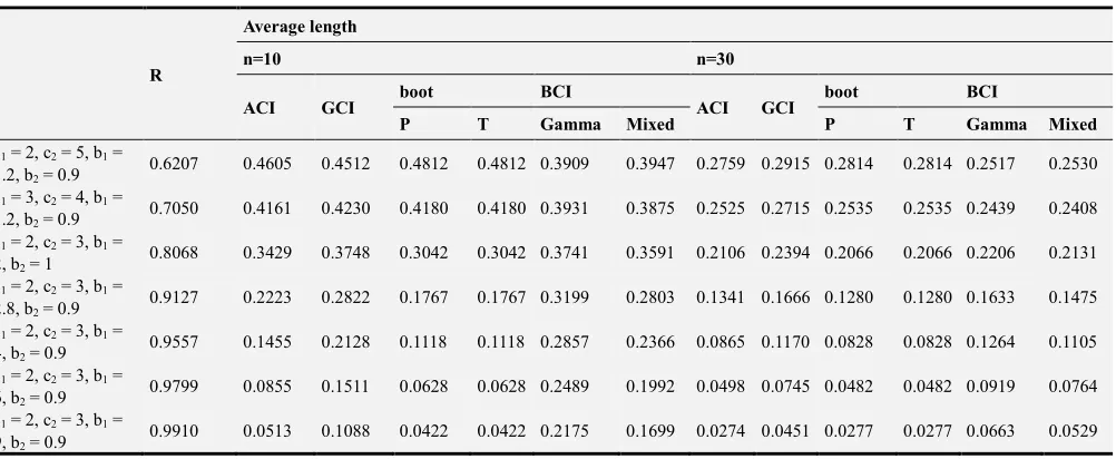
Table 1. Average length of the confidence intervals of R for inverse Weibull distributions, —˜=
™š›š; œ = 1, 2.
R
Average length
n=10 n=30
ACI GCI boot BCI ACI GCI boot BCI
P T Gamma Mixed P T Gamma Mixed
c1 = 2, c2 = 5, b1 =
1.2, b2 = 0.9
0.6207 0.4605 0.4512 0.4812 0.4812 0.3909 0.3947 0.2759 0.2915 0.2814 0.2814 0.2517 0.2530
c1 = 3, c2 = 4, b1 =
1.2, b2 = 0.9
0.7050 0.4161 0.4230 0.4180 0.4180 0.3931 0.3875 0.2525 0.2715 0.2535 0.2535 0.2439 0.2408
c1 = 2, c2 = 3, b1 =
2, b2 = 1
0.8068 0.3429 0.3748 0.3042 0.3042 0.3741 0.3591 0.2106 0.2394 0.2066 0.2066 0.2206 0.2131
c1 = 2, c2 = 3, b1 =
2.8, b2 = 0.9
0.9127 0.2223 0.2822 0.1767 0.1767 0.3199 0.2803 0.1341 0.1666 0.1280 0.1280 0.1633 0.1475
c1 = 2, c2 = 3, b1 =
4, b2 = 0.9
0.9557 0.1455 0.2128 0.1118 0.1118 0.2857 0.2366 0.0865 0.1170 0.0828 0.0828 0.1264 0.1105
c1 = 2, c2 = 3, b1 =
6, b2 = 0.9
0.9799 0.0855 0.1511 0.0628 0.0628 0.2489 0.1992 0.0498 0.0745 0.0482 0.0482 0.0919 0.0764
c1 = 2, c2 = 3, b1 =
9, b2 = 0.9
Table 2. Average coverage probability of the confidence intervals of R for inverse Weibull distributions, —˜=
™š›š; œ = 1, 2.
R
Average coverage probability
n=10 n=30
ACI GCI boot BCI ACI GCI boot BCI
P T Gamma Mixed P T Gamma Mixed
c1 = 2, c2 = 5, b1 =
1.2, b2 = 0.9
0.6207 0.887 0.951 0.884 0.838 0.985 0.973 0.907 0.944 0.904 0.866 0.956 0.945
c1 = 3, c2 = 4, b1 =
1.2, b2 = 0.9
0.7050 0.865 0.942 0.867 0.811 0.954 0.959 0.893 0.941 0.879 0.853 0.924 0.933
c1 = 2, c2 = 3, b1 = 2,
b2 = 1
0.8068 0.835 0.94 0.793 0.746 0.874 0.963 0.874 0.944 0.864 0.82 0.914 0.947
c1 = 2, c2 = 3, b1 =
2.8, b2 = 0.9
0.9127 0.794 0.923 0.732 0.666 0.741 0.915 0.871 0.953 0.846 0.801 0.865 0.937
c1 = 2, c2 = 3, b1 = 4,
b2 = 0.9
0.9557 0.772 0.919 0.718 0.614 0.627 0.879 0.834 0.942 0.826 0.755 0.787 0.907
c1 = 2, c2 = 3, b1 = 6,
b2 = 0.9
0.9799 0.721 0.918 0.688 0.588 0.513 0.809 0.83 0.942 0.835 0.718 0.713 0.861
c1 = 2, c2 = 3, b1 = 9,
b2 = 0.9
0.9910 0.695 0.922 0.681 0.55 0.421 0.71 0.789 0.926 0.801 0.684 0.642 0.82
Table 3. Left tail error of the confidence intervals of R for inverse Weibull distributions, —˜=
™š›š; œ = 1, 2.
R
Left tail error
n=10 n=30
ACI GCI boot BCI ACI GCI boot BCI
P T Gamma Mixed P T Gamma Mixed
c1 = 2, c2 = 5, b1 =
1.2, b2 = 0.9
0.6207 0.2219 0.2540 0.2435 0.2210 0.2373 0.1956 0.1318 0.1536 0.1270 0.1421 0.1416 0.1222
c1 = 3, c2 = 4, b1 =
1.2, b2 = 0.9
0.7050 0.1961 0.2555 0.2145 0.1796 0.2930 0.2282 0.1238 0.1550 0.1212 0.1274 0.1670 0.1331
c1 = 2, c2 = 3, b1 = 2,
b2 = 1
0.8068 0.1658 0.2562 0.1552 0.1376 0.3083 0.2530 0.1035 0.1475 0.0999 0.1031 0.1631 0.1359
c1 = 2, c2 = 3, b1 =
2.8, b2 = 0.9
0.9127 0.1158 0.2240 0.1013 0.0846 0.3016 0.2342 0.0677 0.1152 0.0689 0.0604 0.1384 0.1101
c1 = 2, c2 = 3, b1 = 4,
b2 = 0.9
0.9557 0.0783 0.1816 0.0712 0.0517 0.2821 0.2156 0.0459 0.0883 0.0495 0.0384 0.1156 0.0912
c1 = 2, c2 = 3, b1 = 6,
b2 = 0.9
0.9799 0.0475 0.1363 0.0440 0.0284 0.2516 0.1916 0.0273 0.0604 0.0322 0.0209 0.0885 0.0685
c1 = 2, c2 = 3, b1 = 9,
b2 = 0.9
0.9910 0.0297 0.1019 0.0336 0.0168 0.2224 0.1685 0.0154 0.0384 0.0200 0.0110 0.0656 0.0496
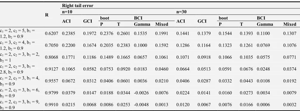
Table 4. Right tail error of the confidence intervals of R for inverse Weibull distributions, —˜=
™š›š; œ = 1, 2.
R
Right tail error
n=10 n=30
ACI GCI boot BCI ACI GCI boot BCI
P T Gamma Mixed P T Gamma Mixed
c1 = 2, c2 = 5, b1 =
1.2, b2 = 0.9
0.6207 0.2385 0.1972 0.2376 0.2601 0.1535 0.1991 0.1441 0.1379 0.1544 0.1393 0.1100 0.1307
c1 = 3, c2 = 4, b1 =
1.2, b2 = 0.9
0.7050 0.2200 0.1674 0.2035 0.2383 0.1000 0.1592 0.1286 0.1164 0.1323 0.1261 0.0769 0.1076
c1 = 2, c2 = 3, b1 = 2,
b2 = 1 0.8068 0.1771 0.1186 0.1489 0.1665 0.0657 0.1061 0.1071 0.0918 0.1066 0.1035 0.0575 0.0771
c1 = 2, c2 = 3, b1 =
2.8, b2 = 0.9
0.9127 0.1065 0.0582 0.0753 0.0920 0.0183 0.0460 0.0664 0.0513 0.0591 0.0676 0.0248 0.0374
c1 = 2, c2 = 3, b1 = 4,
b2 = 0.9
0.9557 0.0672 0.0312 0.0406 0.0601 0.0036 0.0210 0.0406 0.0287 0.0332 0.0443 0.0108 0.0192
c1 = 2, c2 = 3, b1 = 6,
b2 = 0.9 0.9799 0.0379 0.0147 0.0188 0.0344 -0.0026 0.0076 0.0224 0.0141 0.0160 0.0273 0.0034 0.0079
c1 = 2, c2 = 3, b1 = 9,
b2 = 0.9
(iv) Finally, the 1 − α 100% G-BCI and 1 −
α 100%M-BCI of R, are obtained using Algorithm 2. The hyper-parameters of priors for G-BCI and M-BCI are chosen on basis of the same mean but different variances as the follow
G-BCI: let α , β = 2, 4 , α , β = 1, 2 , μ , λ =
pS, 3s, and μ , λ = p , 1s.
M-BCI: let α , β = 2, 4 , and α , β = 1, 2. The comparisons on the basis of average length, average coverage, and left and right tail errors are introduced in Tables (1-4), respectively. From Tables 1-4, the following results are observed:
1.As expected, the average length of all confidence intervals decreases when n and R increase.
2.When R = 0.8068-0.9910, the average length of boot and the left tail error of T-boot are smallest, and the left tail error of all confidence intervals decrease when n and R increase.
3.The average coverage of GCI is approximately around the 1 − α 100%.
4.The average coverage of ACI, boot, and G-BCI decrease when R increases. But the average coverage of ACI and boot increase when n increases.
5.For all the confidence intervals, the right tail error is decreasing when R is increasing. Moreover the right tail error of all confidence intervals except BCI are decreasing when n is increasing.
6.The right tail error of BCI is the smallest.
7. Conclusion
In this article, several approaches for estimating the confidence intervals of Stress-Strength Reliability P(X1 < X2)
are provided when random variables having general inverse exponential form distributions with different unknown parameters. A simulation study is performed to compare its performance using the inverse Weibull distribution as an example of the general inverse exponential form distribution. The comparison is carried out on basis of average length, average coverage, and tail errors. The results obtained were very close to each other.
References
[1] S. Kotz, Y. Lumelskii, M. Pensky, The Stress-Strength Model and its Generalizations: Theory and Applications, Singapore: World Scientific, 2003.
[2] D. Al-Mutairi, M. Ghitany, D. Kunddu, Inferences on stress-strength reliability from Lindley distributions, Communications in Statistics-Theory and Methods, 8 (2013) 1443-1463.
[3] N. Amiri, R. Azimi, F. Yaghmaei, M. Babanezhad, Estimation of stress-strength parameter for two parameter Weibull distribution, International Journal of Advanced Statistics and Probability, 1(2013) 4-8.
[4] S. Rezaei, R. Tahmasbi, M. Mahmoodi, Estimation of P(Y < X) for generalized Pareto distribution, Statistical Planning and Inference, 140 (2010) 480-494.
[5] N. Mokhlis, E. Ibrahim, D. Gharieb, Stress-strength reliability with general form distributions, Communications in Statistics-Theory and Methods, 46 (2017) 1230-1246.
[6] N. Mokhlis, E. Ibrahim, D. Gharieb, Interval estimation of a
P X < X model with general form distributions for unknown parameters, Statistics Applications and Probability, 6 (2017) 391-400.
[7] B. Efron, An Introduction to the Bootstrap, Chapman and Hall, 1994.
[8] A. Asgharzadeh, R. Valiollahi, M. Z. Raqab, Estimation of the stress-strength reliability for the generalized logistic distribution, Statistical Methodology, 15 (2013) 73-94. [9] D. R. Thoman, L. J. Bain, C. E. Antle, Inferences on the
parameters of the Weibull distribution, Technometrics, 11(1969) 445-446.
[10] K. Krishnamoorthy, Y. Lin, Y. Xia, Confidence limits and prediction limits for a Weibull distribution based on the generalized variable approach, Statistical Planning and Inference, 139 (2009) 2675–2684.