Hit Miss Networks with Applications to Instance Selection
Elena Marchiori [email protected]
Department of Computer Science Radboud University
Nijmegen, The Netherlands
Editor: Leon Bottou
Abstract
In supervised learning, a training set consisting of labeled instances is used by a learning algo-rithm for generating a model (classifier) that is subsequently employed for deciding the class label of new instances (for generalization). Characteristics of the training set, such as presence of noisy instances and size, influence the learning algorithm and affect generalization performance. This pa-per introduces a new network-based representation of a training set, called hit miss network (HMN), which provides a compact description of the nearest neighbor relation over pairs of instances from each pair of classes. We show that structural properties ofHMN’s correspond to properties of training points related to the one nearest neighbor (1-NN) decision rule, such as being border or central point. This motivates us to useHMN’s for improving the performance of a1-NN classifier by removing in-stances from the training set (instance selection). We introduce three newHMN-based algorithms for instance selection.HMN-C, which removes instances without affecting accuracy of1-NN on the original training set,HMN-E, based on a more aggressive storage reduction, andHMN-EI, which ap-plies iterativelyHMN-E. Their performance is assessed on 22 data sets with different characteristics, such as input dimension, cardinality, class balance, number of classes, noise content, and pres-ence of redundant variables. Results of experiments on these data sets show that accuracy of1-NN classifier increases significantly whenHMN-EI is applied. Comparison with state-of-the-art editing algorithms for instance selection on these data sets indicates best generalization performance of HMN-EIand no significant difference in storage requirements. In general, these results indicate that HMN’s provide a powerful graph-based representation of a training set, which can be successfully applied for performing noise and redundance reduction in instance-based learning.
Keywords: graph-based training set representation, nearest neighbor, instance selection for
instance-based learning
1. Introduction
A central issue in1-NN classification, and more generally in instance-based learning, concerns storage requirements. The basic1-NN rule stores all training instances, hence can be slow when classifying new instances. Moreover, when the training set contains noisy instances, generalization accuracy can be negatively affected if these instances are stored as well (see Wilson and Martinez, 2000). Instance selection algorithms tackle these issues by selecting a subset of the training set in order to reduce storage and possibly also enhance accuracy of the1-NN rule on new instances (generalization performance).
In this paper we introduce a new graph-based representation of a training set, called Hit Miss Network. In anHMN, nodes are instances of the considered training set. Edges are defined as follows: for each node x and for each class, there is a directed edge from x to its nearest neighbor among training set instances belonging to that class. ThusHMN represents a ’more specific’ nearest neighbor relation, namely between points from each pair of classes. Exact computation ofHMN has quadratic time complexity. This bound can be reduced by using metric trees or other spatial data structures (Grother et al., 1997).
We show that structural properties ofHMN’s correspond to properties of training instances related to the decision boundary of the1-NN rule, such as being border or central point. These observations motivate the use ofHMN for performing instance selection for the1-NN rule. We introduce three new instance selection algorithms. The first algorithm, calledHMN-C, discards instances corresponding to nodes of theHMN with no incoming edges (zero in-degree nodes). We prove that instance selec-tion by means of this algorithm does not change the1-NN classification of instances in the original training set. The second algorithm, called HMN-E, employs a more aggressive deletion strategy, removing a larger number of training instances, including those with zero in-degree. The last al-gorithm, calledHMN-EI, applies iterativelyHMN-E. These algorithms have the desirable properties of being order-independent and of having quadratic time complexity, which can be reduced using metric trees or other spatial data structures.
We assess effectiveness of the proposed algorithms with respect to generalization performance of the1-NN rule and storage requirements, using 22 data sets with different characteristics, such as input dimension, cardinality, class balance, number of classes, noise content, and presence of redun-dant variables. Results of experiments show thatHMN-EI improves significantly average accuracy of the 1-NN rule, and achieves significantly better performance than HMN-C andHMN-E. Experi-ments on the same data sets are conducted with the following three algorithms, which have been analyzed in Brighton and Mellish’s paper on advances in instance selection (Brighton and Mel-lish, 2002). Edited Nearest Neighbor (E-NN), designed for noise reduction (Wilson, 1972), and two state-of-the-art editing algorithms: Iterative Case Filtering (ICF) (Brighton and Mellish, 1999) and the best of the Decremental Reduction Optimization algorithms introduced in Wilson and Martinez (1997) (DROP3). Comparison of the results shows thatHMN-EI achieves best accuracy, with storage requirements similar to those ofICF andDROP3.
These results indicate thatHMN’s provide a powerful graph-based representation of training sets, with local structural graph properties useful for analyzing and enhancing1-NN-based classification.
1.1 Related Work
1-NN instance-based learning mainly use proximity graphs. Proximity graphs are defined as graphs in which points close to each other by some definition of closeness are connected (Barnett, 1976). The nearest neighbor graph (NNG) is a typical example of proximity graph, where each vertex is a data point that is joined by an edge to its nearest neighbor. The minimum spanning tree (MST) is also a proximity graph. Graph-based applications to instance-based learning algorithms mainly use the Gabriel graph (GG). Exact computation of the Gabriel graph is cubic in the number of nodes. Both theNNG andMSTare subgraphs of theGG. TheGGis a subgraph of the Delaunay Triangulation (DT), the dual of the Voronoi diagram. The Voronoi diagram and correspondingly theDTof a point set capture all the proximity information about the point set because they represent the original1-NN rule decision boundary.
There are two main differences between the above proximity graphs and HMN’s. First, HMN’s explicitly use the class label of points in the definition of edges. As a consequence, while the above proximity graphs can be applied to any data set, HMN’s are specifically defined for labeled data. Second,HMN’s are directed graphs, while the above proximity graphs are not.
A class of directed proximity graphs, called class cover catch digraphs (CCCD’s) has been intro-duced in Marchette et al. (2003), which provide a graph-based representation of one (target) class versus a different (non-target) class. In aCCCD of two such classes, nodes are the target instances and the maximal covering balls centered on each target instance, where a maximal covering ball of a target point is the ball centered in that point with maximum radius, which does not contain any non-target point. Each maximal covering ball is connected to its center by a directed edge.
CCCD’s have been used for translating the so-called ’constrained class cover problem’ (CCCP) to a problem on directed graphs. TheCCCPamounts to find a minimum cardinality set of open covering balls with centers in target class points whose union covers the target class and does not contain any point of the non-target class.
The problem of finding an optimal solution to an instance of the CCCPhas been shown to be equivalent to the one of finding a minimum cardinality dominating set in a general digraph. For CCCD’s with points on Euclidean L2 metric space, the problem can be solved in O(nm)time, with n and m equal to the number of target and non-target points, respectively. Further information
about analysis ofCCCD’s and their application to classification can be found in DeVinney and Priebe (2005), DeVinney and Priebe (2006) and D.J. Marchette and Priebe (2005).
While bothHMN’s andCCCD are directed graphs, they describe different relations:HMN’s describe the nearest neighbor relation between points of each pair of classes, while CCCD’s describe the relation between maximal covering balls and target instances of one class.
Representations of a data set based on proximity graphs have been used to define algorithms for reducing the size of the training set (for instance, Bhattacharya, 1982), for removing noisy instances (for instance, S´anchez et al., 1997), and for detecting critical instances close to the decision boundary (for instance, Bhattacharya and Kaller, 1998), in order to improve storage and accuracy of1-NN.
Faster algorithms for instance selection based on theGGand the Reduced Neighborhood graph (Jaromczyk and Toussaint, 1992) have been proposed, for instance in Bhattacharya and Kaller (1998), Bhattacharya et al. (2005), Bhattacharya (1982), Mukherjee (2004) and S ´anchez et al. (1997). In particular, in Bhattacharya et al. (2005) a specific data-structure for efficient compu-tation of approximate Gabriel neighbor is proposed. Moreover, three instance selection algorithms are considered: Gabriel-Graph algorithm,ICF, and a so-called Hybrid. Hybrid incorporatesE-NN, ICF, and the Gabriel graph rule. Specifically, it consists of the sequential application of a modified version of E-NN based on approximate Gabriel neighbor, a condensing step using Gabriel graph rule, and a filtering step ofICF. The authors provide a rather short discussion of results, and do not test the difference in quality of the average results of the algorithms.
For a thorough survey of graph-based methods for nearest neighbor classification, the reader is referred to Toussaint (2002).
The rest of the paper is organized as follows. After introducing the terminology used throughout the paper, the next section defines HMN’s and discusses their properties. Section 3 presents a brief review of instance selection methods. Section 4 introducesHMN-C,HMN-E andHMN-EI. Section 5 describes experiments. Finally, in Section 6, we conclude and point to future work.
1.2 Terminology
The following notions and terms will be used in the sequel. - X : a training set,
- L=1, . . . ,c: class labels of X
- x: an element of X ,
-|X|: the number of elements (cardinality) of X , - Xi: the set of points of X with label i,
- label(x): the class label of x,
-1-NN(x,l): the nearest neighbor of x among those points (different from x) with label l, - G: a directed graph with nodes representing elements of X ,
- e= (x,y): an edge of G, with x the vertex from which e is directed and y the vertex to which e is directed,
- d(x): the number of edges where x occurs (the degree of x), - d(G): the total number of edges of G (the degree of G), - in-degree of x: the number of edges pointing to x,
2. Hit Miss Networks
Suppose X consists of points from c different classes. In anHMN of X , a directed edge from point
x to y is defined if y is the nearest neighbor of x in the class of y. Thus each point x has c outgoing
edges, one for each class. When the classes of x and y are the same, we call x a hit of y, otherwise a
miss of y . The name hit miss network is derived from these terms.
Definition 2.1 (Hit Miss Network) The Hit Miss Network of X ,HMN(X), is a directed graph G= (V,E)with
−1 −0.8 −0.6 −0.4 −0.2 0 0.2 0.4 0.6 0.8 1 −1
−0.8 −0.6 −0.4 −0.2 0 0.2 0.4 0.6 0.8 1
0 0 1 2
1 1 0 1
0 5 3 0 2 0
0 2 1 0
1 0
3 0
0 0
1 0 2 1
0 3 2 1
0 2 1 0
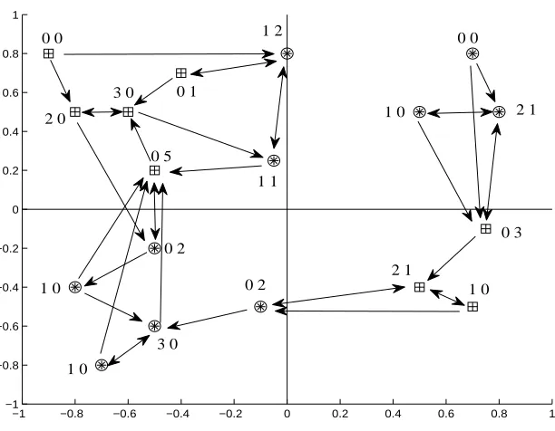
Figure 1: HMN graph of the training set for an artificial classification problem. Hit- and miss-degree of each node is written on the left and right side of the node, respectively.
• E={(x,1-NN(x,l))for each x∈X and l∈L}.
Definition 2.2 (Hit, Miss Points) Let G=HMN(X). A hit of x (respectively, miss of x) is any point y such that e= (y,x)is an edge of G and label(y) =label(x)(respectively, label(y)6=label(x)).
We call hit-degree (respectively miss-degree) of x the number of hit (respectively miss) nodes of x. Hit(x)(respectively Miss(x)) denotes the set of hit (respectively miss) nodes of x.
Figure 1 shows theHMN of the training set for a toy binary classification task. Observe that the two points with zero in-degree are relatively isolated and far from points of the opposite class, while points with high miss-degree are closer to points of the opposite class and to the 1-NN decision boundary.
ComputingHMN requires quadratic time complexity in the number of points. Nevertheless, by using metric trees or other spatial data structures this bound can be reduced. For instance, using
kd trees, whose construction takes time proportional to n log(n), nearest neighbor search exhibits approximately O(n1/2)behavior (Grother et al., 1997). A recent fast all nearest neighbor algorithm for applications involving large point-clouds is introduced in Sankaranarayanan et al. (2007).
By construction, the degree of G, and the degree d(x) of a node x∈V satisfy the following
properties:
and
c≤d(x)≤ |X|+c−1.
HMN’s describe the nearest neighbor relation over pairs of points from each pair of classes of the training set. Formally, it is easy to check that
HMN(X) =∪i,j,i6=j,i,j∈[1,c]HMN(Xi∪Xj).
Therefore, the HMN’s of pairs of classes can be constructed independently, supporting parallel execution. Moreover, if a new class is added, one does not need to reconstruct the entireHMN, but theHMN, between the new class and each of the other ones.
−1 −0.8 −0.6 −0.4 −0.2 0 0.2 0.4 0.6 0.8 1
−1 −0.8 −0.6 −0.4 −0.2 0 0.2 0.4 0.6 0.8 1
0 10 20 30 40 50 60 70 80 90 100
0 2 4 6 8 10 12
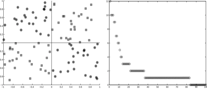
Figure 2: A XOR problem data set (left) and plot of sorted in-degrees (y-axis) of nodes (x-axis), in decreasing order, of the correspondingHMN graph (right).
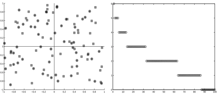
Figure 2 shows a training set for a XOR classification task, and the sorted in-degrees of itsHMN graph. The in-degree distribution seems to follow a Power law, where very few nodes have high in-degree. If we randomly permute the class labels of the training set then the degree distribution changes, with lower in-degree values and more nodes having small in-degree (cf., Figure 3).
These observations indicate that the local structure ofHMN provides information about properties of the training points, and motivate us to useHMN’s for defining a new instance selection technique. Before that, in the next section we review briefly instance selection algorithms.
3. Instance Selection Algorithms
−1 −0.8 −0.6 −0.4 −0.2 0 0.2 0.4 0.6 0.8 1 −1
−0.8 −0.6 −0.4 −0.2 0 0.2 0.4 0.6 0.8 1
0 10 20 30 40 50 60 70 80 90 100
0 1 2 3 4 5 6
Figure 3: Training points of a XOR problem data set with labels randomly permuted (left figure) and plot of in-degrees, sorted in decreasing order, obtained by applyingHMN (right figure).
Instance selection techniques, here also called editing techniques, select a subset of the training set in order to improve the storage and possibly the generalization performance of an instance-based learning algorithm. In this paper we focus on the1-NN classifier.
Research on instance selection started with the seminal work of Hart (1968). Subsequent re-search focussed mainly on three types of training set condensation techniques (Brighton and Mel-lish, 2002): competence preservation, competence enhancement, and hybrid approaches.
• Competence preservation algorithms compute a training set consistent subset by removing
ir-relevant points that do not affect the classification accuracy of the training set (see for instance Angiulli, 2007; Dasarathy, 1994).
• Competence enhancement methods remove noisy points in order to increase classifier
accu-racy. Noise reduction techniques can remove exception instances or border instances which cannot be distinguished from true noise by the technique, hence can possibly affect negatively the generalization performance of the classifier that uses only the selected instances (see for instance Vezhnevets and Barinova, 2007; Wilson, 1972).
• Hybrid methods aim at finding a subset of the training set that is both noise free and does
not contain irrelevant points (for instance, Brighton and Mellish, 2002; Wilson and Martinez, 1997). Alternative methods use prototypes instead of instances of the training set (see for instance Pekalska et al., 2006).
In particular, in Brighton and Mellish (2002) the authors compare experimentally Edited Nearest Neighbor (E-NN) and the state-of-the-art editing algorithms Iterative Case Filtering (ICF) and Decre-mental Reduction Optimization Procedure 3 (DROP3).E-NN is an algorithm generally considered in comparative experimental analysis of editing methods mainly because it provides useful information on the amount of ’noisy’ instances contained in the considered data sets, and on the improvement of accuracy obtained by their removal. Iterative Case Filtering usesE-NN as pre-processing noise reduction step, followed by an iterative procedure for deleting ’superfluous points’. AlsoDROP3 begins with the application of a simple noise reduction step, followed by another simple type of heuristic for discarding ’superfluous points’.
Results of an extensive comparative experimental analysis performed in Wilson and Martinez (2000) and in Brighton and Mellish (2002) indicate thatICF andDROP3 are cutting-edge instance selection algorithms, achieving best K-NN accuracy and storage reduction on a large number of learning tasks over many other editing methods. These algorithms, together with E-NN, are de-scribed in more detail below and used to assess comparatively the performance of theHMN-based editing algorithms we propose.
3.1 Edited Nearest Neighbor
Wilson (1972) introduced the Edited Nearest Neighbor (E-NN), where each point x is removed from
X if it does not agree with the majority of its K nearest neighbors. This editing rule removes noisy
points as well as points close to the decision boundary, yielding to smoother decision boundaries.
3.2 Iterative Case Filtering
In Brighton and Mellish (1999) the Iterative Case Filtering algorithm (ICF) was proposed, which first applies E-NN iteratively until it cannot remove any point, and next iteratively removes other points as follows. At each iteration, all points for which the so-called reachability set is smaller than the coverage one are deleted. The reachability of a point x consists of the points inside the largest hyper-sphere containing only points of the same class as x. The coverage of x is defined as the set of points that contain x in their reachability set.
3.3 Decremental Reduction Optimization
The family of Decremental Reduction Optimization (DROP) algorithms was first introduced by Wil-son and Martinez (1997), and further extended and analyzed in WilWil-son and Martinez (2000). It consists of five algorithmsDROP1-5.DROP1is the basic removal rule, which removes a point x from
X if the accuracy of theK-NNrule on the set of its associates does not decrease. Each point has a list of K nearest neighbors and a list of associates, which are updated each time a point is removed from
X . A point y is an associate of x if x belongs to the set of K nearest neighbors of y. If x is removed
then the list of K nearest neighbors of each of its associates y is updated by adding a new neighbor point z, and y is added to the list of associates of z. Moreover, for each of the K nearest neighbors y of x, x is removed from the list of associates of y.
neighbor from the other classes (nearest enemy). In this way, points furthest from their nearest enemy are selected first.
DROP3applies a pre-processing step which discards points of X misclassified by their K nearest neighbors, and then appliesDROP2.
DROP4uses a stronger pre-processing step which discards points of X misclassified by their K nearest neighbors if their removal does not hurt the classification of other instances.
Finally DROP5modifies DROP2by considering the reverse order of selection of points, in such a way that instances are considered for removal beginning with instances that are nearest to their nearest enemy.
DROP3 achieves the best mix of storage reduction and generalization accuracy of theDROP meth-ods (see Wilson and Martinez, 2000). Moreover, results of experiments conducted in Wilson and Martinez (1997, 2000) show thatDROP3 achieves higher accuracy and smaller storage requirements than several other methods, such as CNN (Hart, 1968), SNN (Ritter et al., 1975), E-NN (Wilson, 1972), theAll k-NNmethod (Tomek, 1976),IB2, IB3(Aha et al., 1991), and theExploremethod (Cameron-Jones, 1995). Therefore we useDROP3 andICF as representatives of the state-of-the-art, in order to assess the performance of theHMN-based editing algorithms introduced in the following section.
4. Instance Selection with Hit Miss Networks
Zero in-degree nodes ofHMN(X)include relatively isolated points, and points not too close to the decision boundary. This is illustrated in theHMN-Csub-plot of Figure 5, where zero in-degree nodes of theHMN for a XOR data set are highlighted in bold.
Zero in-degree nodes can be safely removed from X without affecting1-NN classification of the original training. Formally, we have the following result.
Proposition 4.1 Let S be obtained by removing from X all points with zero in-degree. Then S is a decision-boundary consistent subset.
Proof
Suppose there exists x∈X s.t. 1-NN(x,X) =y, 1-NN(x,S) =y1 and l(y)6=l(y1). Then y6=y1 and y has been removed. So y has in-degree equal to 0.
From 1-NN(x,X) =y it follows that x is in Hit(y)or in Miss(y), hence the in-degree of y is at least 1, which yields a contradiction.
Then l(y)6=l(y1)was false. Hence S is a training set consistent subset.
We callHMN-C (HMN for training set Consistent instance selection) the algorithm that removes from the training set all instances with zero in-degree.
HMN-C does not remove noisy instances, which are in general close to the class decision bound-ary. Therefore, a more aggressive removal strategy is adopted in the following instance selection heuristic algorithm, calledHMN-E (HMN for Editing), which compares the hit- and miss-degree of each node for deciding whether to remove it.
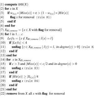
(1)computeHMN(X) (2)for x in X
(3) if wl(x)∗ |Miss(x)|+ε>(1−wl(x))∗ |Hit(x)|
(4) flag x for removal (rule R1) (5) end if
(6)end for
(7)XR1,remove={x∈X with flag for removal} (8)for l in 1. . .c
(9) Le f tl ={x6∈XR1,remove|l(x) =l} (10) if|Le f tl|<4
(11) unflag{z∈XR1,remove|l(z) =l,in-degree(z)>0}(rule R2) (12) end if
(13)end for
(14)for x in XR1,remove
(15) if c>3 and|Miss(x)|<c/2 and in-degree(x)>0 (16) unflag x(rule R3)
(17) end if
(18) if|Hit(x)| ≥ |Xl(x)|/4
(19) unflag x(rule R4) (20) end if
(21)end for
(22)remove from X all x with flag for removal
Figure 4: Pseudo-code ofHMN-E algorithm. Input: training set X . Output: subset of X .
1. The first rule removes x if its miss-degree is greater or equal than its hit-degree, that is
|Miss(x)| ≥ |Hit(x)|. This amounts to discard a point when it is isolated (that is, has zero in-degree), as well as when it has more ’miss’ than ’hit’ points.
In order to deal with unbalanced data sets, the terms of the inequality are weighted by the fraction of points of the same and other classes, respectively, resulting in ruleR1(lines 3-5 in Figure 1) which removes a point x from X if
wl(x)∗ |Miss(x)|+ε>(1−wl(x))∗ |Hit(x)|, (1)
where wl(x)=|{z|l(z) =l(x)}|/|X|andε<1 (ε=0.1 is used in our experiments).
2. On small data sets, application of R1could remove too many points of one class. Rule R2 (lines 10-12 in Figure 1) handles this case. It checks if the size of a class becomes too small after application ofR1. In such a case all points of that class having positive in-degree are added. The threshold used in the rule is set in such a way that the minimum size of a condensed class becomes equal to 4. We consider this to be a reasonable class storage lower bound for the condensed1-NN rule.
3. Suppose for simplicity each class has equal size (|X|/c). Then|Miss(x)| ≤ (c−1c)2|X|, and
classes, while the|Hit(x)|’s upper bound depends on c in an inversely linear way. Therefore
|Miss(x)|is more likely to grow faster than|Hit(x)|in the presence of many classes. This justifies the introduction of the heuristic RuleR3(lines 15-17 in Figure 1), which deals with data sets having more than three classes. For more than three classes, a point x with in-degree greater than 0 is added if it has a low number of ’miss’ points, low with respect to c. Here we use as threshold half of the total number of classes.
4. Points with many ’hits’ are closer to the ’centroid’ of the class, hence are considered to be relevant for discriminating the classes, even when they are close to points of other classes. This case is implemented in ruleR4(lines 18-20 in Figure 1) which adds x if it is the ’hit’ of at least 25% of the points of its class.
Rules R2 - R4are ’rules of thumb’. The threshold in each of these rules has been fixed to a value considered reasonable, and has not been tuned on each specific data set. These rules could be improved by means of parameter tuning or domain knowledge on the specific data distribution of the learning task.
In order to remove more “redundant” points,HMN-E can be applied iteratively as follows: repeat the application ofHMN-E until the generalization accuracy of1-NN on the original training set with the reduced set decreases. We call this algorithmHMN-E Iterated (HMN-EI).
Observe that the threeHMN-based editing algorithms are order independent, that is, their output does not depend on the order in which training points are processed. Moreover, by construction, points removed by HMN-C are also removed by HMN-E, and points removed by HMN-E are also removed byHMN-EI.
4.1 Comparison of the Methods on the XOR Problem
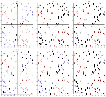
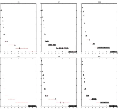
Figure 5 shows application of the considered editing algorithms to the training set of a XOR classi-fication task. Points removed by an algorithm are shown in bold. As expected, points removed by E-NN are close to the decision boundary.ICF andDROP3 delete also ’safe’ points far from the deci-sion boundary (in order to enhance storage requirements).HMN-C removed points ’locally’ isolated, whileHMN-E removes also ’safe’ points as well as points close to the decision boundary. Its iterated versionHMN-EI selects very few points far from the decision boundary. The figures do not show any other apparent set-theoretic relationship between the subsets of points removed by the methods. Figure 6 plots the sorted in-degrees of the considered XOR training set, where in-degree of points removed by a method are marked with triangles. As expected, points removed byICF and not already deleted byE-NN have low in-degree. The majority of points removed byE-NN have high in-degree, showing the tendency of ’noisy’ points to have high in-degree. HMN-E removes more points with high in-degree thanE-NN, and it selects points with low, but not zero, degree. While HMN-EI selects only points with in-degree 1 and 2, ICF andDROP3 select also points of higher degree. On this example,HMN-EI achieves best storage reduction.
5. Experiments
−1 −0.8 −0.6 −0.4 −0.2 0 0.2 0.4 0.6 0.8 1 −1 −0.8 −0.6 −0.4 −0.2 0 0.2 0.4 0.6 0.8 1 ENN
−1 −0.8 −0.6 −0.4 −0.2 0 0.2 0.4 0.6 0.8 1 −1 −0.8 −0.6 −0.4 −0.2 0 0.2 0.4 0.6 0.8 1 ICF
−1 −0.8 −0.6 −0.4 −0.2 0 0.2 0.4 0.6 0.8 1 −1 −0.8 −0.6 −0.4 −0.2 0 0.2 0.4 0.6 0.8 1 DROP3
−1 −0.8 −0.6 −0.4 −0.2 0 0.2 0.4 0.6 0.8 1 −1 −0.8 −0.6 −0.4 −0.2 0 0.2 0.4 0.6 0.8 1 HMN−C
−1 −0.8 −0.6 −0.4 −0.2 0 0.2 0.4 0.6 0.8 1 −1 −0.8 −0.6 −0.4 −0.2 0 0.2 0.4 0.6 0.8 1 HMN−E
−1 −0.8 −0.6 −0.4 −0.2 0 0.2 0.4 0.6 0.8 1 −1 −0.8 −0.6 −0.4 −0.2 0 0.2 0.4 0.6 0.8 1 HMN−EI
Figure 5: Effect of the algorithms on a XOR problem training set: removed points are shown with filled markers. Top row, from left to right: E-NN,ICF,DROP3. Bottom row, from left to right:HMN-C,HMN-E andHMN-EI.
algorithms and conducted extensive experiments on 22 Machine Learning benchmark data sets. All algorithms are tested using one neighbor.
The performance measures here used are (average) test accuracy of the classifier and (average) percentage of the training set removed by the method.
5.1 Data Sets
0 10 20 30 40 50 60 70 80 90 100 0 2 4 6 8 10 12 14 ENN
0 10 20 30 40 50 60 70 80 90 100
0 2 4 6 8 10 12 14 ICF
0 10 20 30 40 50 60 70 80 90 100
0 2 4 6 8 10 12 DROP3
0 10 20 30 40 50 60 70 80 90 100
0 2 4 6 8 10 12 14 HMNC
0 10 20 30 40 50 60 70 80 90 100
0 2 4 6 8 10 12 14 HMNE
0 10 20 30 40 50 60 70 80 90 100
0 2 4 6 8 10 12 14 HMN−EI
Figure 6: In-degree of nodes of theHMN built on the considered XOR training set, sorted in decreas-ing order. The in-degree of points removed by an algorithm are marked with triangles. Top row, from left to right: E-NN, ICF,DROP3. Bottom row, from left to right: HMN-C, HMN-E andHMN-EI.
1. Raetsch’s binary classification benchmark data sets have been used in R ¨atsch et al. (2001): they consists of 1 artificial and 12 real-life data sets from the UCI, DELVE and STATLOG benchmark repositories.
For each experiment, the 100 (20 for Splice andImage) partitions of each data set into training and test set available in the repository are here used.
Bayes’ error is 5%. In contrast,g10nis a deterministic problem in 10 dimensions, where the decision function traverses the centers of the Gaussians, and depends on only two of the input dimensions.
The three real world data sets areCoil20, consisting of gray-scale images of 20 different objects taken from different angles, in steps of 5 degrees, Uspst, the test data part of the USPS data on handwritten digit recognition, andText consisting of the classes ’mac’ and ’mswindows’ of the Newsgroup20 data set.
For each experiment, the 10 partitions of each data set into training and test set available in the repository are used.
3. Finally, we consider four standard benchmark data sets from the UCI Machine Learning repository:Iris,Bupa,Pima, andBreast-W.
For each experiment, 100 partitions of each data set into training and test set are used. Each partition randomly divides the data set into training and test set, equal to 80% and 20% of the data, respectively.
Thus the benchmark data consists of 3 artificial data sets (Banana, g50c, g10n) and 19 real-life ones, with different characteristics as shown in Table 1. In particular, Chapelle’s data sets are balanced, that is, all classes are represented by similar number of points, while some of Raetsch’s data sets are rather unbalanced.
5.2 Results
Cross validation is applied to each data set. For each partition of the data set, each editing algorithm is applied to the training set X from which a subset S is returned. The one nearest neighbor classifier that uses only points of S is applied to the test set. The average accuracy on the test set over the given partitions is reported for each algorithm (cf., Table 2, Table 3). The average percentage of instances that are excluded from S is also reported under the column with label R. Average and median accuracy and training set reduction percentage for each algorithm over all the 22 data sets is reported near the bottom of the Table.
We compare statisticallyHMN-EI with each of the other algorithms as follows.
• First a paired t-test on the cross validation results on each data set is applied, to assess whether the average accuracy forHMN-EI is significantly different than each of the other algorithms. In Tables 2, 3 a ’+’ indicates thatHMN-EI’s average accuracy is significantly higher than the other algorithm at a 0.05 significance level. Similarly, a ’-’ indicates thatHMN-EI’s average accuracy is significantly lower than the other algorithm at a 0.05 significance level. The row labeled ’Sig.acc.+/-’ reports the number of timesHMN-EI’s average accuracy is significantly better and worse than each of the other algorithms at a 0.05 significance level. A paired t-test is also applied to assess significance of differences in storage reduction percentages for each experiment.
Data Set CL VA TR Cl.Inst. TE Cl.Inst.
Banana 2 2 400 212-188 4900 2712-2188
B.Cancer 2 9 200 140-60 77 56-21
Diabetis 2 8 468 300-168 300 200-100
German 2 20 700 478-222 300 222-78
Heart 2 13 170 93-77 100 57-43
Image 2 18 1300 560-740 1010 430-580
Ringnorm 2 20 400 196-204 7000 3540-3460
F.Solar 2 9 666 293-373 400 184-216
Splice 2 60 1000 525-475 2175 1123-1052
Thyroid 2 5 140 97-43 75 53-22
Titanic 2 3 150 104-46 2051 1386-66
Twonorm 2 20 400 186-214 7000 3511-3489
Waveform 2 21 400 279-121 4600 3074-1526
g50 2 50 550 252-248 50 23-27
g10n 2 10 550 245-255 50 29-21
Coil20 20 1024 1440 70 40 2
Text 2 7511 1946 959-937 50 26-24
Uspst 10 256 2007 267-201-169-192-137 50 6-5-9-4-3-3-4-5-5 -171-169-155-175
Iris 3 4 120 40-40-40 30 10-10-10
Bupa 2 6 276 119-157 69 26-43
Pima 2 8 615 398-217 153 102-51
Breast-W 2 9 546 353-193 137 91-46
Table 1: Data Sets used in the experiments. Raetsch’s benchmark repository available at http://ida.first.fraunhofer.de/projects/bench/benchmarks.htm. Chapelle’s one at http://www.kyb.tuebingen.mpg.de/bs/people/chapelle/lds/. Four pop-ular benchmark data sets from UCI Machine Learning repository available at http://mlearn.ics.uci.edu/MLRepository.html. CL = number of classes, TR = training set, TE = test set, VA = number of variables, Cl.Inst. = number of instances in each class.
(respectively ’-’) in the row labeled ’Wilcoxon’ indicates thatHMN-EI is significantly better (respectively worse) than the other algorithm.
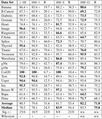
Results of Table 2 show thatHMN-EI achieves best generalization accuracy, significantly better than the one of 1-NN and of HMN-C. Moreover, HMN-EI outperforms significantly HMN-E with respect to storage requirements and achieves similar generalization performance. For these reasons, HMN-EI is chosen for further comparison with state-of-the-art editing algorithms.
5.3 Comparison with Other Algorithms
Data Set 1-NN HMN-C R HMN-E R HMN-EI R Banana 86.4 + 85.6 + 19.7 + 88.2 + 38.5 + 88.6 57.9 B.Cancer 67.3 + 65.9 + 20.1 + 66.1 + 50.0 + 69.2 72.8 Diabetis 69.9 + 68.6 + 22.4 + 72.5 + 53.1 + 73.5 73.1 German 70.5 + 69.4 + 26.0 + 72.5 56.4 + 72.9 75.5 Heart 76.8 + 76.1 + 23.7 + 81.7 52.9 + 81.6 79.3 Image 96.6 - 96.1 - 23.7 + 94.8 - 41.1 + 92.7 57.3 Ringnorm 65.0 + 63.4 + 33.5 + 66.6 - 63.9 + 65.6 82.9 F.Solar 60.8 + 60.5 + 80.1 + 63.5 + 86.9 + 64.7 92.1 Splice 71.1 - 70.1 + 46.0 + 72.3 - 71.7 + 70.7 86.6 Thyroid 95.6 - 94.9 - 24.2 + 93.4 38.9 + 93.2 59.1 Titanic 67.0 + 66.9 + 79.6 + 70.9 + 84.9 + 76.0 94.7 Twonorm 93.3 + 92.8 + 39.4 + 95.7 60.4 + 95.9 83.5 Waveform 84.2 + 83.6 + 36.2 + 86.0 - 58.0 + 85.4 79.9 g50c 79.6 + 80.2 + 42.7 + 87.4 - 71.0 + 86.8 88.3 g10n 75.0 + 74.6 + 26.0 + 75.8 + 63.5 + 79.2 82.5 Coil20 100 - 100 - 6.7 + 100 - 10.4 + 99.5 15.0
Text 92.8 - 90.8 - 16.7 + 89.4 - 54.1 + 86.4 78.9
Uspst 94.6 - 94.6 - 12.5 + 94.4 - 20.3 + 93.6 29.8 Iris 95.5 95.0 24.7 + 95.1 38.7 + 95.4 75.2 Breast-W 95.7 + 95.5 + 50.7 + 97.1 54.9 + 96.9 71.8 Bupa 61.6 + 59.5 + 18.5 + 63.4 + 54.7 + 64.5 76.0 Pima 67.8 + 66.5 + 21.4 + 70.8 + 50.8 + 71.7 68.1
Average 80.3 79.6 31.6 81.7 53.4 82.2 71.8
Median 78.2 78.1 24.5 83.9 54.4 83.5 75.8
Sig.+/- 15/6 16/5 22/0 8/8 22/0 n/a n/a
Wilcoxon + + + ∼ + n/a n/a
Table 2: Results of experiments on ML benchmark data sets. Each column labeled with the name of an algorithm reports its average test set accuracy on each data set. R = percentage of training points removed. Best results are shown in bold. Average (Median) = average (median) results over data sets. Sig.+/- = number of timesHMN-EI average accuracy (stor-age reduction) is significantly better (+) or significantly worse (-) than the other algorithm, according to a paired t-test at 0.05 significance level. Wilcoxon = a ’+’ indicatesHMN-EI significantly better than the other algorithm at a 0.01 significance level according to a Wilcoxon test for paired samples,∼indicates no significant difference.
Data Set HMN-EI R ICF R E-NN R DROP3 R Banana 88.6 57.9 86.1 + 79.2 - 87.8 + 13.1 + 87.6 + 68.2 -B.Cancer 69.2 72.8 67.0 + 79.0 - 69.4 33.3 + 69.7 - 72.9 Diabetis 73.5 73.1 69.8 + 83.1 - 72.6 + 30.3 + 72.3 + 73.4 German 72.9 75.5 68.6 + 82.2 - 73.0 30.1 + 72.0 + 74.3 + Heart 81.6 79.3 76.7 + 80.9 - 80.6 + 23.1 + 80.2 + 72.1 + Image 92.7 57.3 93.8 80.3 - 95.8 - 3.4 + 95.1 - 64.9 -Ringnorm 65.6 82.9 61.2 + 85.5 - 54.8 + 35.3 + 54.7 + 80.6 + F.Solar 64.7 92.1 61.0 + 52.0 + 61.3 + 39.8 + 61.4 + 93.8
-Splice 70.7 86.6 66.3 + 85.5 + 68.4 + 28.3 + 67.6 + 79.01 + Thyroid 93.2 59.1 91.9 + 85.6 - 94.0 - 4.0 + 92.7 + 65.7 -Titanic 76.0 94.7 67.5 54.3 + 67.3 + 33.0 + 67.7 + 94.3 Twonorm 95.9 83.5 89.2 + 90.7 - 94.1 + 6.4 + 94.3 + 72.7 + Waveform 85.4 79.9 82.1 86.8 - 85.4 15.7 + 84.9 + 73.6 + g50c 86.8 88.3 82.2 + 56.3 + 82.2 + 19.7 + 82.8 + 77.7 + g10n 79.2 82.5 73.0 + 53.9 + 74.0 + 22.8+ 75.0 + 71.4 + Coil20 99.5 15.0 98.5 + 42.6 - 100 - 0.0 + 95.5 + 64.4 -Text 86.4 78.9 88.2 - 68.8 + 91.6 - 7.7 + 88.0 - 66.7 + Uspst 93.6 29.8 86.2 87.8 - 94.0 4.7 + 91.4 + 67.3 -Iris 95.4 75.2 95.3 69.7 + 95.9 - 4.2 + 95.8 - 66.4 + Breast-W 96.9 71.8 95.4 + 93.8 - 96.6 4.1 + 96.8 74.2 -Bupa 64.5 76.0 60.9 + 74.3 + 63.2 + 38.1+ 63.1 + 73.8 + Pima 71.7 68.1 67.9 + 78.7 - 69.7 + 32.4 + 69.4 + 73.3
-Average 82.0 71.8 78.6 75.0 80.5 19.5 79.9 73.7
Median 83.5 75.8 79.4 79.8 81.4 21.25 81.5 73.1
Sig.+/- n/a n/a 16/2 7/15 12/5 22/0 17/4 11/8
Wilcoxon n/a n/a + ∼ + + + ∼
Table 3: Results of experiments on ML benchmark data sets ofHMN-EI,ICF, Wilson’s editing, and DROP3.
• On theg10ndata set,HMN-EI achieves significantly better performance than that of the other methods, indicating robustness to the presence of irrelevant variables (on this type of classifi-cation task).
• On data sets with more than three classes,HMN-EI has worse storage requirements than the other algorithms, but also generally higher accuracy, due to the more conservative editing strategy (Rule 3)HMN-EI uses on data sets with many classes.
ICF, according to this test. As shown, for instance, in Demsar (2006), comparison of the performance of two algorithms based on the t-test is only indicative because the assumptions of the test are not satisfied, and the Wilcoxon test is shown to provide more reliable estimates.
• Results of the non parametric Wilcoxon test for paired samples at a 0.01 significance level indicate that the performance of HMN-EI on the entire set of classification tasks is signifi-cantly better than each one of the other algorithms with respect to accuracy, and that there is no significant difference in storage reduction betweenHMN-EI and state-of-the-art editing algorithms (cf., last row of the table).
• The three best performing instance selection algorithms,DROP3,ICF andHMN-EI have quadratic computational complexity in the number of instances (which can be reduced by using ad-hoc data structures such as kd-trees). ICF andHMN-EI are in principle slower than the other algorithms, due to their multiple passes over (selected) instances. Nevertheless, in our ex-periments these algorithms require a small number of iterations (about 7 forICF and 3 for HMN-EI). Thus their computational complexity is not significantly worse than that ofDROP3.
In summary, results of these experiments indicate effectiveness ofHMN-based instance selection and robustness ofHMN-EI with respect to the presence of high number of variables, training exam-ples, multiple classes, noise and irrelevant variables. Comparison with results obtained by E-NN, ICF andDROP3 shows improved average accuracy and similar storage requirement ofHMN-EI,ICF andDROP3 on these data sets.
6. Conclusions and Future Work
This paper proposed a new graph-based representation of a training set and showed how local struc-tural properties of nodes provide information about the closeness of the corresponding points to the decision boundary of the1-NN rule. We formalized these properties by means of the notions of Hit and Miss set, and used such notions for defining three algorithms for1-NN’s instance selection. We proved thatHMN-C removes instances without affecting the accuracy of the1-NN rule on the orig-inal training set (it computes a decision-boundary consistent subset). We showed thatHMN-E and HMN-EI remove more points thanHMN-C, including those close to the decision boundary. Results of extensive experiments indicated thatHMN-EI significantly improves the generalization accuracy of 1-NN and reduces significantly its storage requirements.
We compared experimentallyHMN-EI with a popular noise reduction algorithm (E-NN), and two state-of-the-art editing algorithms (ICF andDROP3). Results of extensive experiments on 19 real-life data sets and 3 artificial ones showed thatHMN-EI achieved best average accuracy, and storage reduction similar to that ofICF andDROP3. This indicates that simple local topological properties of the proposed graph-based data set representation provide an effective tool for 1-NN’s instance selection.
In this paper we use only the degree of nodes as mean for analyzing a training set in order to im-proving1-NN’s performance. It would be interesting to investigate whether other graph-theoretical properties ofHMN’s, such as information on path distance, clustering coefficient and diameter, pro-vide useful information for studying and improving the1-NN’s performance.
Other future work includes the use ofHMN’s to tackle the following interesting problems: mea-suring the difficulty of a learning task with respect to a given training set (see for instance Zighed et al., 2002); enhancing classification techniques based on a notion of margin, such as Support Vec-tor Machines (see for instance Shin and Cho, 2007); improving Boosting algorithms by means of editing techniques (see for instance Vezhnevets and Barinova, 2007), and, more generally, tackling over-fitting in supervised learning.
Acknowledgments
Many thanks to the Reviewers and to the Editor Leon Bottou for their constructive comments.
References
D.W. Aha, D. Kibler, and M.K. Albert. Instance-based learning algorithms. Machine Learning, 6: 37–66, 1991.
F. Angiulli. Fast nearest neighbor condensation for large data sets classification. IEEE Transactions
on Knowledge and Data Engineering, 19(11):1450–1464, 2007. ISSN 1041-4347.
V. Barnett. The ordering of multivariate data. J. Roy. Statist. Soc., Ser. A 139(3):318–355, 1976.
B. Bhattacharya and D. Kaller. Reference set thinning for the k-nearest neighbor decision rule.
Proceedings of the 14th International Conference on Pattern Recognition, (1):238–243, 1998.
B. Bhattacharya, K. Mukherjee, and G. Toussaint. Geometric decision rules for instance-based learning problems. In Proceedings of the 1st International Conference on Pattern Recognition
and Machine Intelligence (PReMI’05), number LNCS 3776, pages 60–69. Springer, 2005.
B.K. Bhattacharya. Application of computational geometry to pattern recognition problems. PhD
Thesis. Simon Fraser University, School of Computing Science, Technical Report, TR 82-3, 1982.
H. Brighton and C. Mellish. On the consistency of information filters for lazy learning algorithms. In PKDD ’99: Proceedings of the Third European Conference on Principles of Data Mining and
Knowledge Discovery, pages 283–288. Springer-Verlag, 1999.
H. Brighton and C. Mellish. Advances in instance selection for instance-based learning algorithms.
Data Mining and Knowledge Discovery, (6):153–172, 2002.
R.M. Cameron-Jones. Instance selection by encoding length heuristic with random mutation hill climbing. In Proceedings of the Eighth Australian Joint Conference on Artificial Intelligence, pages 99–106, 1995.
O. Chapelle and A. Zien. Semi-supervised classification by low density separation. In Proceedings
T. Cover and P. Hart. Nearest neighbor pattern classification. IEEE Transactions on Information
Theory, 13:21–27, 1967.
B. V. Dasarathy. Minimal consistent set (mcs) identification for optimal nearest neighbor decision systems design. IEEE Transactions on Systems, Man, and Cybernetics, 24(3):511–517, 1994.
J. Demsar. Statistical comparisons of classifiers over multiple data sets. Journal of Machine
Learn-ing Research, 7:1–30, 2006.
J. DeVinney and C.E. Priebe. The use of domination number of a random proximity catch digraph for testing spatial patterns of segregation and association. Statistics and Probability Letters, 73 (1):37–50, 2005.
J. DeVinney and C.E. Priebe. A new family of proximity graphs: Class cover catch digraphs.
Discrete Applied Mathematics, 154(14):1975–1982, 2006.
E.J. Wegman D.J. Marchette and C.E. Priebe. Fast algorithms for classification using class cover catch digraphs. Handbook of Statistics, 24:331–358, 2005.
S.N. Dorogovtsev and J.F.F. Mendes. Evolution of Networks: From Biological Nets to the Internet
and WWW. Oxford University Press, 2003.
P.J. Grother, G.T. Candela, and J.L. Blue. Fast implementation of nearest neighbor classifiers.
Pattern Recognition, 30:459–465, 1997.
P. E. Hart. The condensed nearest neighbor rule. IEEE Transactions on Information Theory, 14: 515–516, 1968.
N. Jankowski and M. Grochowski. Comparison of instances selection algorithms i. algorithms survey. In Artificial Intelligence and Soft Computing, pages 598–603. Springer, 2004a.
N. Jankowski and M. Grochowski. Comparison of instances selection algorithms ii. results and comments. In Artificial Intelligence and Soft Computing, pages 580–585. Springer, 2004b.
J.W. Jaromczyk and G.T. Toussaint. Relative neighborhood graphs and their relatives. P-IEEE, 80: 1502–1517, 1992.
C.D.J. Marchette, C.E. Priebe, D.A. Socolinsky, and J.G. DeVinney. Classification using class cover catch digraphs. Journal of classification, 20(1):3–23, 2003.
K. Mukherjee. Application of the gabriel graph to instance-based learning. In M.sc. project, School
of Computing Science, Simon Fraser University, 2004.
E. Pekalska, R.P. W. Duin, and P. Pacl´ık. Prototype selection for dissimilarity-based classifiers.
Pattern Recognition, 39(2):189–208, 2006.
G. R¨atsch, T. Onoda, and K.-R. M ¨uller. Soft margins for AdaBoost. Machine Learning, 42(3): 287–320, 2001.
J.S. S´anchez, F. Pla, and F.J. Ferri. Prototype selection for the nearest neighbour rule through proximity graphs. Pattern Recognition Letters, 18:507–513, 1997.
J. Sankaranarayanan, H. Samet, and A. Varshney. A fast all nearest neighbor algorithm for applica-tions involving large point-clouds. Comput. Graph., 31(2):157–174, 2007.
H. Shin and S. Cho. Neighborhood property based pattern selection for support vector machines.
Neural Computation, (19):816–855, 2007.
I. Tomek. An experiment with the edited nearest-neighbor rule. IEEE Transactions on Systems,
Man, and Cybernetics, 6(6):448–452, 1976.
G.T. Toussaint. Proximity graphs for nearest neighbor decision rules: recent progress. In
Interface-2002, 34th Symposium on Computing and Statistics, pages 83–106, 2002.
G.T. Toussaint, B.K. Bhattacharya, and R.S. Poulsen. The application of voronoi diagrams to non-parametric decision rules. In Proceedings of the 16th Symposium on Computer Science and
Statistics, pages 97 –108, 1984.
A. Vezhnevets and O. Barinova. Avoiding boosting overfitting by removing ”confusing” samples. In Proceedings of the 18th European Conference on Machine Learning (ECML), volume 4701, pages 430–441. LNCS, 2007.
D. L. Wilson. Asymptotic properties of nearest neighbor rules using edited data. IEEE Transactions
on Systems, Man and Cybernetics, (2):408–420, 1972.
D.R. Wilson and T.R. Martinez. Instance pruning techniques. In Proc. 14th International
Confer-ence on Machine Learning, pages 403–411. Morgan Kaufmann, 1997.
D.R. Wilson and T.R. Martinez. Reduction techniques for instance-based learning algorithms.
Ma-chine Learning, 38(3):257–286, 2000.
D.A. Zighed, S. Lallich, and F. Muhlenbach. Separability index in supervised learning. In PKDD