Least-Squares Policy Iteration
Michail G. Lagoudakis [email protected]
Ronald Parr [email protected]
Department of Computer Science Duke University
Durham, NC 27708, USA
Editor:Peter L. Bartlett
Abstract
We propose a new approach to reinforcement learning for control problems which com-bines value-function approximation with linear architectures and approximate policy iter-ation. This new approach is motivated by the least-squares temporal-difference learning algorithm (LSTD) for prediction problems, which is known for its efficient use of sample experiences compared to pure temporal-difference algorithms. Heretofore, LSTD has not had a straightforward application to control problems mainly because LSTD learns the state value function of a fixed policy which cannot be used for action selection and control without a model of the underlying process. Our new algorithm, least-squares policy itera-tion (LSPI), learns the state-acitera-tion value funcitera-tion which allows for acitera-tion selecitera-tion without a model and for incremental policy improvement within a policy-iteration framework. LSPI is a model-free, off-policy method which can use efficiently (and reuse in each iteration) sample experiences collected in any manner. By separating the sample collection method, the choice of the linear approximation architecture, and the solution method, LSPI allows for focused attention on the distinct elements that contribute to practical reinforcement learning. LSPI is tested on the simple task of balancing an inverted pendulum and the harder task of balancing and riding a bicycle to a target location. In both cases, LSPI learns to control the pendulum or the bicycle by merely observing a relatively small number of trials where actions are selected randomly. LSPI is also compared againstQ-learning (both with and without experience replay) using the same value function architecture. While LSPI achieves good performance fairly consistently on the difficult bicycle task,Q-learning variants were rarely able to balance for more than a small fraction of the time needed to reach the target location.
Keywords: Reinforcement Learning, Markov Decision Processes, Approximate Policy Iteration, Value-Function Approximation, Least-Squares Methods
1. Introduction
standpoint. When linear methods fail, it is usually relatively easy to get some insight into why the failure has occurred.
Our enthusiasm for the approach presented in this paper is inspired by theleast-squares temporal-differencelearning algorithm (LSTD) (Bradtke and Barto, 1996). The LSTD algo-rithm is ideal for prediction problems, that is, problems where we are interested in learning the value function of a fixed policy. LSTD makes efficient use of data and converges faster than other conventional temporal-difference learning methods. However, LSTD heretofore has not had a straightforward application to control problems, that is, problems where we are interested in learning a good control policy to achieve a task. Although it is initially appealing to attempt to use LSTD in the evaluation step of a policy-iteration algorithm, this combination can be problematic. Koller and Parr (2000) present an example where the combination of LSTD-style function approximation and policy iteration oscillates between two very bad policies in an MDP with just 4 states (Figure 9). This behavior is explained by the fact that linear approximation methods such as LSTD compute an approximation that is weighted by the state visitation frequencies of the policy under evaluation.1 Further, even if this problem is overcome, a more serious difficulty is that the state value function that LSTD learns is of no use for policy improvement when a model of the process is not available, which is the case for most reinforcement-learning control problems.
This paper introduces theleast-squares policy-iteration(LSPI) algorithm, which extends the benefits of LSTD to control problems. First, we introduce LSTDQ, an algorithm simi-lar to LSTD that learns the approximatestate-action value functionof a fixed policy, thus permitting action selection and policy improvement without a model. Then, we introduce LSPI which uses the results of LSTDQto form an approximate policy-iteration algorithm. LSPI combines the policy-search efficiency of policy iteration with the data efficiency of LSTDQ. LSPI is a completely off-policy algorithm and can, in principle, use data col-lected arbitrarily from any reasonable sampling distribution. The same data are (re)used in each iteration of LSPI to evaluate the generated policies. LSPI enjoys the stability and soundness of approximate policy iteration and eliminates learning parameters, such as the learning rate, that need careful tuning. We evaluate LSPI experimentally on several con-trol problems. A simple chain walk problem is used to illustrate important aspects of the algorithm and the value-function approximation method. LSPI is tested on the simple task of balancing an inverted pendulum and the harder task of balancing and riding a bicycle to a target location. In both cases, LSPI learns to control the pendulum or the bicycle by merely observing a relatively small number of trials where actions are selected randomly. We also compare LSPI to Q-learning (Watkins, 1989), both with and without experience replay (Lin, 1993), using the same value function architecture. While LSPI achieves good performance fairly consistently on the difficult bicycle task,Q-learning variants were rarely able to balance the bicycle for more than a small fraction of the time needed to reach the target location.
The paper is organized as follows: first, we provide some background on Markov de-cision processes (Section 2) and approximate policy iteration (Section 3); after outlining the main idea behind LSPI (Section 4) and discussing value-function approximation with
linear architectures (Section 5), we introduce LSTDQ (Section 6) and LSPI (Section 7); next, we compare LSPI to other reinforcement-learning methods (Section 8) and present an experimental evaluation and comparison (Section 9); finally, we discuss open questions and future directions of research (Section 10).
2. Markov Decision Processes
We assume that the underlying control problem is a Markov decision process (MDP). An MDP is defined as a 5-tuple (S,A,P, R, γ) where: S = {s1, s2, ..., sn} is a finite set of states; A = {a1, a2, ..., am} is a finite set of actions; P is a Markovian transition model, where P(s, a, s0) is the probability of making a transition to state s0 when taking action a in states(s−→a s0);R:S × A × S 7→IR is a reward (or cost) function, such thatR(s, a, s0) is the reward for the transition s −→a s0; and, γ ∈ [0,1) is the discount factor for future rewards. For simplicity of notation, we defineR:S × A 7→IR, the expected reward for a state-action pair (s, a), as:
R(s, a) = X s0∈S
P(s, a, s0)R(s, a, s0) .
We will be assuming that the MDP has an infinite horizon and that future rewards are discounted exponentially with the discount factor (assuming that all policies are proper, that is, they reach a terminal state with probability 1, our results generalize to the undiscounted case,γ = 1, as well).
A stationary policy π for an MDP is a mappingπ :S 7→Ω(A), where Ω(A) is the set of all probability distributions overA;π(a;s) stands for the probability that policyπ chooses action ain states. A stationary deterministic policyπ is a policy that commits to a single action choice per state, that is, a mappingπ :S 7→ A from states to actions; in this case,
π(s) indicates the action that the agent takes in states.
The state-action value function Qπ(s, a) of any policy π is defined over all possible combinations of states and actions and indicates the expected, discounted, total reward when taking actionain state sand following policyπ thereafter:
Qπ(s, a) =Eat∼π;st∼P
∞ X
t=0
γtrt
s0=s, a0=a !
.
The exact Qπ values for all state-action pairs can be found by solving the linear system of the Bellman equations:
Qπ(s, a) =R(s, a) +γ X s0∈S
P(s, a, s0) X a0∈A
π(a0;s0)Qπ(s0, a0) .
In matrix format, the system becomes
Qπ =R+γPΠπQπ ,
where Qπ and R are vectors of size |S||A|, P is a stochastic matrix of size (|S||A| × |S|) that contains the transition model of the process,
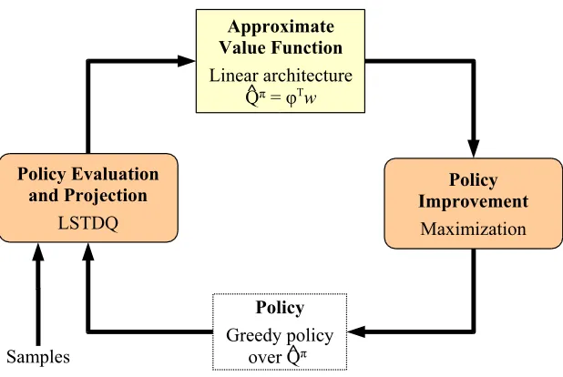
Figure 1: Policy Iteration (Actor-Critic Architecture)
and Ππ is a stochastic matrix of size (|S| × |S||A|) that describes policyπ,
Ππ s0,(s0, a0)
=π(a0;s0) .
The resulting linear system,
(I−γPΠπ)Qπ =R ,
can be solved analytically or iteratively to obtain the exact Qπ values. The state-action value functionQπ is also the fixed point of the Bellman operator T
π:
(TπQ)(s, a) =R(s, a) +γ X
s0∈S
P(s, a, s0) X a0∈A
π(a0;s0)Q(s0, a0) .
Tπ is a monotonic and quasi-linear operator and a contraction mapping in the L∞ norm with contraction rateγ (Bertsekas and Tsitsiklis, 1996). For any initial vectorQ, successive applications of Tπ converge to the state-action value function Qπ of policyπ.
For every MDP, there exists an optimal deterministic policy, π∗, which maximizes the expected, total, discounted reward from any initial state. It is, therefore, sufficient to restrict the search for the optimal policy only within the space of deterministic policies.
3. Policy Iteration and Approximate Policy Iteration
Policy iteration(Howard, 1960) is a method of discovering the optimal policy for any given MDP. Policy iteration is an iterative procedure in the space of deterministic policies; it discovers the optimal policy by generating a sequence of monotonically improving policies. Each iteration m consists of two phases: policy evaluation computes the state-action value functionQπmof the current policyπ
mby solving the linear system of the Bellman equations, and policy improvement defines the improved greedy policy πm+1 over Qπm as
πm+1(s) = arg max a∈A
Qπm(s, a) .
Figure 2: Approximate Policy Iteration
in the policy in which case the iteration has converged to the optimal policy, often in a surprisingly small number of iterations. Policy improvement is also know as the actor
and policy evaluation is known as the critic, because the actor is responsible for the way the agent acts and the critic is responsible for criticizing the way the agent acts. Hence, policy-iteration algorithms are also refered to as actor-critic architectures (Barto et al., 1983; Sutton, 1984). Figure 1 shows a block diagram of policy iteration (or an actor-critic architecture) and the dependencies among the various components.
The guaranteed convergence of policy iteration to the optimal policy relies heavily upon a tabular representation of the value function, exact solution of the Bellman equations, and tabular representation of each policy. Such exact representations and methods are impractical for large state and action spaces. In such cases, approximation methods are used. Approximations in the policy-iteration framework can be introduced at two places:2
• The representation of the value function: The tabular (exact) representation of the real-valued functionQπ(s, a) is replaced by a generic parametric function approxima-torQbπ(s, a;w), whereware the adjustable parameters of the approximator.
• The representation of the policy: The tabular (exact) representation of the policy
π(s) is replaced by a parametric representation bπ(s;θ), where θ are the adjustable parameters of the representation.
In either case, only the parameters of the representation need to be stored (along with a compact representation of the approximation architecture) and the storage requirements are much smaller than the tabular case. The crucial factor for a successful approximate algorithm is the choice of the parametric approximation architecture(s) and the choice of the projection (parameter adjustment) method(s). This form of policy iteration (depicted in Figure 2) is known as approximate policy iteration. Notice that policy evaluation and
value-function projection are essentially blended into one procedure, because there is no in-termediate representation of a full value function that would facilitate their separation. The same also is true for policy improvement and policy projection, since there is no interme-diate representation for a complete policy. These facts demonstrate the difficulty involved in the use of approximate methods within policy iteration: off-the-self architectures and projection methods cannot be applied blindly; they have to be fully integrated into the policy-iteration framework.
A natural concern is whether the sequence of policies and value functions generated by an approximate policy-iteration algorithm converges to a policy and a value function that are not far from the optimal ones, if it converges at all. The answer to this question is given by the following generic theorem, adapted from Bertsekas and Tsitsiklis (1996), which shows that approximate policy iteration is a fundamentally sound algorithm: if the error in policy evaluation and projection and the error in policy improvement and projection are bounded, then approximate policy iteration generates policies whose performance is not far from the optimal performance. Further, this difference diminishes to zero as the errors decrease to zero.
Theorem 3.1 Let πb0, πb1, bπ2, ..., bπm be the sequence of policies generated by an
approx-imate policy-iteration algorithm and let Qbπ0b , Qbπ1b , Qbπ2b , ..., Qbπbm be the corresponding ap-proximate value functions. Let and δ be positive scalars that bound the error in all ap-proximations (over all iterations) to value functions and policies respectively. If
∀m= 0,1,2, ..., kQbbπm−Qbπmk
∞≤ ,
and 3
∀m= 0,1,2, ..., kTbπm+1Qb
b
πm−T
∗Qbπbmk∞≤δ .
Then, this sequence eventually produces policies whose performance is at most a constant multiple of and δ away from the optimal performance:
lim sup m→∞ k
b
Qπbm−Q∗k
∞≤
δ+ 2γ
(1−γ)2 .
In addition to thisL∞-norm bound, Munos (2003) recently provided a stronger bound in terms of a weightedL2-norm for a version of approximate policy iteration that involves exact representations of policies and approximate representations of their state value functions and uses the full model of the MDP in both policy evaluation and policy improvement. This recent result provides further evidence that approximate policy iteration is a fundamentally sound algorithm.
3.T∗is theBellman optimality operatordefined as:
(T∗Q)(s, a) =R(s, a) +γ
X
s0∈S
P(s, a, s0) max
a0∈AQ(s 0
Figure 3: Least-squares policy iteration.
4. Reinforcement Learning and Approximate Policy Iteration
For many practical control problems, the underlying MDP model is not fully available. Typically, the state space, the action space, and the discount factor are available, whereas the transition model and the reward function are not known in advance. It is still desirable to be able to evaluate, or, even better, find good decision policies for such problems. However, in this case, algorithms have to rely on information that comes from interaction between the decision maker and the process itself or from a generative model of the process and includes observations of states, actions, and rewards.4 These observations are commonly organized in tuples known as samples:
(s, a, r, s0) ,
meaning that at some time step the process was in states, actionawas taken by the agent, a rewardr was received, and the resulting next state was s0. The problem of evaluating a given policy or discovering a good policy from samples is know as reinforcement learning.
Samples can be collected from actual (sequential) episodes of interaction with the process or from queries to a generative model of the process. In the first case, the learning agent does not have much control on the distribution of samples over the state space, since the process cannot be reinitialized at will. In contrast, with a generative model the agent has full control on the distribution of samples over the state space as queries can be made for any arbitrary state. However, in both cases, the action choices of the learning agent are not restricted by the process, but only by the learning algorithm that is running. Samples may even come from stored experiences of other agents on the same MDP.
The proposed least-squares policy iteration(LSPI) algorithm is an approximate policy-iteration algorithm that learns decision policies from samples. Figure 3 shows a block
4. A generative model of an MDP is a simulator of the process, that is, a “black box” that takes a state
s and an action a as inputs and generates a reward r and a next state s0
diagram of LSPI that demonstrates how the algorithm fits within the approximate policy-iteration framework. The first observation is that the state-action value function is ap-proximated by a linear architecture and its actual representation consists of a compact description of the basis functions and a set of parameters. A key idea in the development of the algorithm was that the technique used by Q-learning of implicitly representing a policy as a state-action value function could be applied to an approximate policy-iteration algorithm. In fact, the policy is not physically stored anywhere, but is computed only on demand. More specifically, for any query state s, one can access the representation of the value function, compute all action values in that state, and perform the maximization to derive the greedy action choice at that state. As a result, all approximations and errors in policy improvement and representation are eliminated at the cost of some extra optimization for each query to the policy.
The missing part for closing the loop is a procedure that evaluates a policy using samples and produces its approximate value function. In LSPI, this step is performed by LSTDQ, an algorithm which is very similar to LSTD and learns efficiently the approximate state-action value functionQbπ of a policyπ when the approximation architecture is a linear architecture. LSPI is only one particular instance of a family of reinforcement-learning algorithms for control based on approximate policy iteration. The two components that vary across instances of this family are the approximation architecture and the policy evaluation and projection procedure. For LSPI, these components were chosen to be linear architectures and LSTDQ, but, in principle, any other pair of choices would produce a reasonable learning algorithm for control. The choices made for LSPI offer significant advantages and opportu-nities for optimizing the overall efficiency of the algorithm.
The following three sections describe all the details of the LSPI algorithm. In Section 5 we discuss linear approximation architectures and two projection methods for such archi-tectures in isolation of the learning problem. We also compare these projection methods and discuss their appropriateness in the context of learning. In Section 6, we describe in detail the LSTDQalgorithm for learning the least-squares fixed-point approximation of the state-action value function of a policy. We also cite a comparison of LSTDQ with LSTD and we present some optimized variants of LSTDQ. Finally, in Section 7 we formally state the LSPI algorithm and discuss its properties.
5. Value-Function Approximation using Linear Architectures
LetQbπ(s, a;w) be an approximation toQπ(s, a) represented by aparametric approximation
architecture with freeparameters w. The main idea of value-function approximation is that the parameters w can be adjusted appropriately so that the approximate values are “close enough” to the original values, and, therefore, Qbπ can be used in place of the exact value functionQπ. The characterization “close enough” accepts a variety of interpretations in this context and it does not necessarily refer to a minimization of some norm. Value-function approximation should be regarded as a functional approximation rather than as a pure
that maximize the accuracy of the approximation according to certain criteria and with respect to the target function. Typically, for ordinary function approximation, this is done using a training set of examples of the form(s, a), Qπ(s, a) that provide the valueQπ(s, a) of the target function at certain sample points (s, a), a problem known assupervised learning. Unfortunately, in the context of decision making, the target function (Qπ) is not known in advance, and must be inferred from the observed system dynamics. The implication is that policy evaluation and projection to the approximation architecture must be blended together. This is usually achieved by trying to find values for the free parameters so that the approximate function has certain properties that are “similar” to those of the original value function.
A common class of approximators for value-function approximation is the so calledlinear architectures, where theQπ values are approximated by a linear parametric combination of
kbasis functions (features):
b
Qπ(s, a;w) = k X
j=1
φj(s, a)wj ,
where the wj’s are the parameters. The basis functions φj(s, a) are fixed, but arbitrary and, in general, non-linear, functions ofsanda. We require that the basis functionsφj are linearly independent to ensure that there are no redundant parameters and that the matrices involved in the computations are full rank.5 In general,k |S||A|and the basis functions
φj have compact descriptions. As a result, the storage requirements of a linear architecture are much smaller than those of the tabular representation. Typical linear approximation architectures are polynomials of any degree (each basis function is a polynomial term) and radial basis functions (each basis function is a Gaussian with fixed mean and variance).
Linear architectures have their own virtues: they are easy to implement and use, and their behavior is fairly transparent, both from an analysis standpoint and from a debugging and feature engineering standpoint. It is usually relatively easy to get some insight into the reasons for which a particular choice of features succeeds or fails. This is facilitated by the fact that the magnitude of each parameter is related to the importance of the corresponding feature in the approximation (assuming normalized features).
Let Qπ be the (unknown) value function of a policy π given as a column vector of size |S||A|. Let also Qbπ be the vector of the approximate state-action values as computed by a linear approximation architecture with parameterswj and basis functionsφj,j= 1,2, ..., k. Define φ(s, a) to be the column vector of size k where each entry j is the corresponding basis functionφj computed at (s, a):
φ(s, a) =
φ1(s, a)
. . . φ2(s, a)
. . . φk(s, a)
.
Now, Qbπ can be expressed compactly as
b
Qπ =Φwπ ,
wherewπ is a column vector of lengthk with all parameters andΦis a (|S||A| ×k) matrix of the form
Φ=
φ(s1, a1)|
. . . φ(s, a)|
. . . φ(s|S|, a|A|)|
.
Each row of Φ contains the value of all basis functions for a certain pair (s, a) and each column of Φ contains the value of a certain basis function for all pairs (s, a). If the basis functions are linearly independent, then the columns ofΦare linearly independent as well. We seek to find a combined policy evaluation and projection method that takes as input a policyπ and the model of the process and outputs a set of parameterswπ such that Qbπ is a “good” approximation to Qπ.
5.1 Bellman Residual Minimizing Approximation
Recall that the state-action value function Qπ is the solution of the Bellman equation:
Qπ =R+γPΠπQπ .
An obvious approach to deriving a good approximation is to require that the approximate value function satisfies the Bellman equation as closely as possible. Substituting the approx-imation Qbπ in place of Qπ yields an overconstrained linear system over thek parameters
wπ:
b
Qπ ≈ R+γPΠπQbπ Φwπ ≈ R+γPΠπΦwπ
(Φ−γPΠπΦ)wπ ≈ R .
Solving this overconstrained system in the least-squares sense yields a solution
wπ =(Φ−γPΠπΦ)|(Φ−γPΠπΦ)−1(Φ−γPΠπΦ)|R ,
that minimizes theL2 norm of the Bellman residual (the difference between the left-hand side and the right-hand side of the Bellman equation) and can be called theBellman residual minimizing approximation to the true value function. Note that the solution wπ of the system is unique since the columns of Φ (the basis functions) are linearly independent by definition. Alternatively, it may be desirable to control the distribution of function approximation error. This can be achieved by solving the system above in a weighted least-squares sense. Letµbe a probability distribution over (s, a) such that the probability
∆µ to be a diagonal matrix with entries µ(s, a), the weighted least-squares solution of the system would be:
wπ =(Φ−γPΠ
πΦ)|∆µ(Φ−γPΠπΦ) −1
(Φ−γPΠπΦ)|∆µR ,
The Bellman residual minimizing approach has been proposed (Schweitzer and Seidmann, 1985) as a means of computing approximate state value functions from the model of the process.
5.2 Least-Squares Fixed-Point Approximation
Recall that the state-action value functionQπ is also the fixed point of the Bellman operator:
TπQπ =Qπ .
Another way to go about finding a good approximation is to force the approximate value function to be a fixed point under the Bellman operator:
TπQbπ ≈Qbπ .
For that to be possible, the fixed point has to lie in the space of approximate value functions which is the space spanned by the basis functions. Even though Qbπ lies in that space by definition,TπQbπ may, in general, be out of that space and must be projected. Considering the orthogonal projection (Φ(Φ|Φ)−1Φ|) which minimizes the L
2 norm, we seek an ap-proximate value functionQbπ that is invariant under one application of the Bellman operator
Tπ followed by orthogonal projection:
b
Qπ = Φ(Φ|Φ)−1Φ| T
πQbπ
= Φ(Φ|Φ)−1Φ| R+γPΠ
πQbπ
.
Note that the orthogonal projection to the column space of Φ is well-defined because the columns ofΦ(the basis functions) are linearly independent by definition. Manipulating the equation above, we derive an expression for the desired solution that amounts to solving a (k×k) linear system, where kis the number of basis functions:
Φ(Φ|Φ)−1Φ|(R+γPΠπQbπ) = Qbπ
Φ(Φ|Φ)−1Φ|(R+γPΠπΦwπ) = Φwπ
Φ (Φ|Φ)−1Φ|(R+γPΠ
πΦwπ)−wπ
= 0 (Φ|Φ)−1Φ|(R+γPΠ
πΦwπ)−wπ = 0 (Φ|Φ)−1Φ|(R+γPΠ
πΦwπ) = wπ Φ|(R+γPΠπΦwπ) = Φ|Φwπ
Φ|(Φ−γPΠπΦ)
| {z } (k×k)
wπ = Φ|R
| {z } (k×1)
.
For anyΠπ, the solution of this system
wπ =Φ|(Φ−γPΠ
πΦ) −1
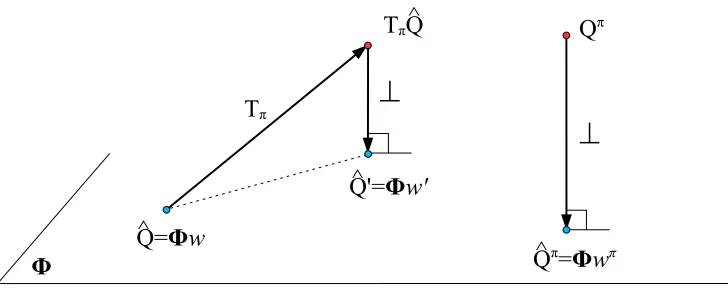
Figure 4: Policy evaluation and projection methods.
is guaranteed to exist for all, but finitely many, values ofγ (Koller and Parr, 2000). Since the orthogonal projection minimizes theL2norm, the solutionwπ yields a value functionQbπ which can be called the least-squares fixed-point approximation to the true value function.
Instead of using the orthogonal projection, it is possible to use a weighted projection to control the distribution of approximation error. Ifµis a probability distribution over (s, a) and ∆µis the diagonal matrix with the projection weightsµ(s, a), the weighted least-squares fixed-point solution would be:
wπ =Φ|∆
µ(Φ−γPΠπΦ) −1
Φ|∆
µR .
The least-squares fixed-point approach has been used for computing (Koller and Parr, 2000) or learning (Bradtke and Barto, 1996) approximate state value functions from a factored model of the process and from samples respectively.
5.3 Comparison of Projection Methods
We presented above two intuitive ways to combine policy evaluation and value-function projection for finding a good approximate value function represented as a linear architecture. An obvious question at this point is whether one of them has some advantages over the other. Figure 4 is a very simplified graphical representation of the situation. Let the three-dimensional space be the space of exact value functionsQand let the two-dimensional space marked byΦbe the space of approximate value functions. Consider the approximate value functionQb=Φwthat lies on Φ. The application of the Bellman operatorTπ to Qb yields a value function TπQb which may be, in general, outside the Φplane. Orthogonal projection (⊥) of TπQb to the Φ plane yields some other approximate value functionQb0 =Φw0. The true value function Qπ of policy π may lie somewhere outside theΦ plane, in general, and its orthogonal projection to the Φplane is marked byQbπ =Φwπ.
the L2 distance between Qb and TπQb, whereas the least-squares fixed-point approximation minimizes the projection of that distance, that is, the distance between Qb and Qb0. In fact, the least-squares fixed-point approximation drives the distance between Qb and Qb0 to zero since it is solving for the fixed point Qb =Qb0. The solution found by the Bellman residual minimizing method will most likely not be a fixed point even within theΦplane.
The Bellman operatorTπ is known to be a contraction in theL∞ norm. In our picture, that means that for any pointQin the three-dimensional space, the pointTπQwill be closer toQπ in theL
∞norm sense. Pictorially, imagine a cube aligned with the axes of the three-dimensional space and centered atQπ withQbeing a point on the surface of the cube; the point TπQwill have to be strictly contained inside this cube (except atQπ where the cube degenerates to a single point). With this view in mind, the Bellman residual minimizing approximation finds the point on the Φ plane where the Bellman operator is making the least progress towardQπ only in terms of magnitude (L
2 distance), ignoring the direction of the change. The motivation for reducing theL2 norm of the Bellman residual comes from the well-known results bounding the distance to Qπ in terms of the L
∞ norm (Williams and Baird, 1993).
On the other hand, the least-squares fixed-point approximation ignores the magnitude of the Bellman operator steps and focuses on the direction of the change. In particular, it solves for the unique point on theΦplane where the Bellman operator becomes perpendicular to the plane. A motivation for choosing this approximation is that if subsequent applications of the Bellman operator point in a similar direction, the approximation should not be far from the projection ofQπ onto theΦplane.
Clearly, the solutions found by these two methods will be different since their objectives are different, except in the case where the true value function Qπ lies in the Φ plane; in that case, both methods are in fact solving the Bellman equation and their solutions are identical. If Qπ does not lie in theΦ plane, there is no clear evidence that any of the two methods will find a good solution or even the solutionwπ that corresponds to the orthogonal projection ofQπ to the plane.
Munos (2003) provides a theoretical comparison of the two approximation methods in the context of state value-function approximation when the model of the process is known. He concludes that the least-squares fixed point approximation is less stable and less predictable compared to the Bellman residual minimizing approximation depending on the value of the discount factor. This is expected, however, since the least-squares fixed-point linear system is singular for a finite number of discount-factor values. On the other hand, he states that the least-squares fixed-point method might be preferable in the context of learning.
From a practical point of view, there are two sources of evidence that the least-squares fixed-point method is preferable to the Bellman residual minimizing method:
• Learning the Bellman residual minimizing approximation requires “doubled” sam-ples (Sutton and Barto, 1998) that can only be collected from a generative model of the MDP.
For the rest of the paper, we focus only on the least-squares fixed-point approximation with minimal reference to the Bellman residual minimizing approximation.
6. LSTDQ: Least-Squares Temporal-Difference Learning for the State-Action Value Function
Consider the problem of learning the (weighted) least-squares fixed-point approximation b
Qπ to the state-action value function Qπ of a fixed policy π from samples. Assuming that there are k linearly independent basis functions in the linear architecture, this problem is equivalent to learning the parameters wπ of Qbπ =Φwπ. The exact values for wπ can be computed from the model by solving the (k×k) linear system
Awπ =b ,
where
A=Φ|∆
µ(Φ−γPΠπΦ) and b=Φ|∆µR ,
and µis a probability distribution over (S × A) that defines the weights of the projection. For the learning problem,Aandbcannot be determineda priori, either because the matrix P and the vector R are unknown, or because P and R are so large that they cannot be used in any practical computation. However, A and b can be learned using samples;6 the learned linear system can then be solved to yield the learned parametersweπ which, in turn, determine the learned value function. Taking a closer look at Aand b:
A = Φ|∆
µ(Φ−γPΠπΦ)
= X s∈S
X
a∈A
φ(s, a)µ(s, a)φ(s, a)−γ X
s0∈S
P(s, a, s0)φ s0, π(s0)|
= X s∈S
X
a∈A
µ(s, a)X s0∈S
P(s, a, s0)
φ(s, a)φ(s, a)−γφ s0, π(s0)|
,
b = Φ|∆
µR
= X s∈S
X
a∈A
φ(s, a)µ(s, a)X s0∈S
P(s, a, s0)R(s, a, s0)
= X s∈S
X
a∈A
µ(s, a)X s0∈S
P(s, a, s0)hφ(s, a)R(s, a, s0)i .
From these equations, it is clear that A and b have a special structure. A is the sum of many rank one matrices of the form:
φ(s, a)φ(s, a)−γφ s0, π(s0)| ,
and bis the sum of many vectors of the form:
φ(s, a)R(s, a, s0) .
These summations are taken overs,a, ands0 and each summand is weighted by the projec-tion weightµ(s, a) for the pair (s, a) and the probabilityP(s, a, s0) of the transitions−→a s0. For large problems, it is impractical to compute this summation over all (s, a, s0) triplets. It is practical, however, to sample terms from this summation; for unbiased sampling, s and
amust be drawn jointly from µ, ands0 must be drawn from P(s, a, s0). It is trivial to see that, in the limit, the process of sampling triplets (s, a, s0) from this distribution and adding the corresponding terms together, can be used to obtain arbitrarily close approximations to A andb.
The key observation here is that a sample (s, a, r, s0) drawn from the process along with the policyπ in states0 provide all the information needed to form one sample term of these summations. This is true because s0 is a sample transition for taking action a in state s, and r is sampled from R(s, a, s0). So, given any finite set of samples,7
D=n (si, ai, ri, s0i)
i= 1,2, . . . , Lo ,
A andb can be learned as:
e
A = 1
L
L X
i=1
φ(si, ai)
φ(si, ai)−γφ s0i, π(s0i) |
,
eb = 1
L
L X
i=1 h
φ(si, ai)ri i
,
assuming that the distribution µD of the samples in D over (S × A) matches the desired distributionµ. The equations can also be written in matrix notation. Let Φe, PΠ^πΦ, and
e
Rbe the following matrices:
e Φ=
φ(s1, a1)| .. .
φ(si, ai)| .. .
φ(sL, aL)|
, PΠ^πΦ=
φ s01, π(s01)|
.. .
φ s0
i, π(s0i) |
.. .
φ s0
L, π(s0L) |
, Re =
r1 .. . ri .. . rL .
Then,Ae andebcan be written as
e A= 1
LΦe |
(Φe −γPΠ^πΦ) and eb= 1
LΦe |
e R .
These two equations show clearly the relationship ofAe andebto Aandb. In the limit of an infinite number of samples,Ae andebconverge to the matrices of the least-squares fixed-point approximation weighted byµD:
lim
L→∞Ae =Φ
|∆
µD(Φ−γPΠπΦ) and lim
L→∞eb=Φ
|∆
µDR .
As a result, the learned approximation is biased by the distribution µD of samples. In general, the distributionµD might be different from the desired distributionµ. A mismatch betweenµandµD may be mitigated by using density estimation techniques to estimate µD and then using projection weights corresponding to the importance weights needed to shift the sampling distribution towards the target distribution. Also, the problem is resolved trivially when a generative model is available, since samples can be drawn so thatµD =µ. For simplicity, this paper focuses only on learned approximations that are naturally biased by the distribution of samples whatever that might be.
In any practical computation of Ae and eb, L is finite and therefore the multiplicative factor (1/L) can be dropped without affecting the solution of the system, since it cancels out. Given that a single sample contributes toAe andebadditively, it is easy to construct an incremental update rule forAe andeb. Let Ae(t) andeb(t) be the current learned estimates of A and bfor a fixed policy π, assuming that initially Ae(0) =0 andeb(0) =0. A new sample (st, at, rt, s0t) contributes to the approximation according to the following update equations:
e
A(t+1)=Ae(t)+φ(st, at)
φ(st, at)−γφ s0t, π(s0t) |
,
eb(t+1) =eb(t)+φ(st, at)rt .
It is straightforward now to construct an algorithm that learns the weighted least-squares fixed-point approximation of the state-action value function of a fixed policyπfrom samples in a batch or in an incremental way. We call this new algorithm LSTDQ (summarized in Figure 5) due to its similarity to LSTD. In fact, one can think of the LSTDQalgorithm as the LSTD algorithm applied on a Markov chain with states (s, a) in which transitions are influenced by both the dynamics of the original MDP and the policyπ being evaluated.
Another feature of LSTDQis that the same set of samples D can be used to learn the approximate value function Qbπ of any policy π, as long as π(s0) is available for each s0 in the set. The policy merely determines which φ s0, π(s0) is added to Ae for each sample. This feature is particularly important in the context of policy iteration since all policies produced during the iteration can be evaluated using a singlesample set.
The approximate value function learned by LSTDQ is biased by the distribution of samples over (S × A). This distribution can be easily controlled when samples are drawn from a generative model, but it is a lot harder when samples are drawn from the actual process. A nice feature of LSTDQis that it poses no restrictions on how actions are chosen during sample collection. Therefore, the freedom in action choices can be used to control the sample distribution to the extent this is possible. In contrast, action choices for LSTD must be made according to the policy under evaluation when samples are drawn from the actual process.
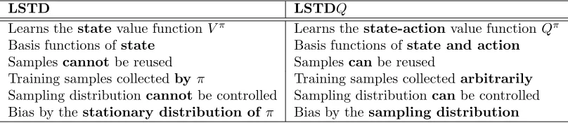
The differences between LSTD and LSTDQare listed in Table 1. The last three items in the table apply only to the case where samples are drawn from the actual process, but there is no difference in the generative model case.
LSTDQ(D, k, φ, γ, π) // LearnsQbπ
from samples
// D : Source of samples(s, a, r, s0
) // k : Number of basis functions // φ : Basis functions
// γ : Discount factor
// π : Policy whose value function is sought
e
A←0 // (k×k) matrix
eb←0 // (k×1) vector
for each (s, a, r, s0)∈D e
A←Ae +φ(s, a)φ(s, a)−γφ s0
, π(s0
)|
eb←eb+φ(s, a)r
e wπ
←Ae−1e
b
returnweπ
Figure 5: The LSTDQ algorithm.
LSTD LSTDQ
Learns thestatevalue functionVπ Learns thestate-actionvalue function Qπ
Basis functions ofstate Basis functions ofstate and action Samplescannotbe reused Samplescanbe reused
Training samples collectedby π Training samples collectedarbitrarily Sampling distributioncannotbe controlled Sampling distributioncanbe controlled Bias by thestationary distribution ofπ Bias by thesampling distribution
Table 1: Differences between LSTD and LSTDQ.
the system and finding the parameters. There is also a cost for determiningπ(s0) for each sample. This cost depends on the specific form of policy representation used.8
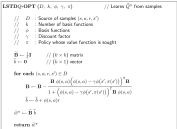
The LSTDQ algorithm in its simplest form involves the inversion of Ae for solving the linear system. However, Ae will not be full rank until a sufficient number of samples has been processed. One way to avoid such singularities is to initialize Ae to a multiple of the identity matrixδIfor some small positiveδ, instead of0 (ridge regression, Dempster et al., 1977). The convergence properties of the algorithm are not affected by this change (Nedi´c and Bertsekas, 2003). Another possibility is to use singular value decomposition (SVD) for robust inversion ofAe which also eliminates singularities due to linearly dependent basis functions. However, if the linear system must be solved frequently and efficiency is a concern, a more efficient implementation of LSTDQ would use recursive least-squares techiques to compute the inverse of Ae recursively. Let B(t) be the inverse of Ae(t) at time t. Using the 8. The explicit tabular representation of π that incurs only a constant O(1) cost per query is not an
LSTDQ-OPT (D, k, φ, γ, π) // LearnsQbπ
from samples
// D : Source of samples(s, a, r, s0
) // k : Number of basis functions // φ : Basis functions
// γ : Discount factor
// π : Policy whose value function is sought
e
B←1
δI // (k×k) matrix
eb←0 // (k×1) vector
for each (s, a, r, s0)∈D
B←B−
Bφ(s, a)φ(s, a)−γφ s0
, π(s0
)|B 1 +φ(s, a)−γφ s0, π(s0)|Bφ(s, a) eb←eb+φ(s, a)r
e wπ
←Beeb
returnweπ
Figure 6: An optimized implementation of the LSTDQalgorithm.
Sherman-Morrison formula, we have:
B(t) = Ae(t−1)+φ(st, at)
φ(st, at)−γφ s0t, π(s0t)
|−1
= B(t−1)−
B(t−1)φ(st, at)
φ(st, at)−γφ s0t, π(s0t) |
B(t−1) 1 +φ(st, at)−γφ s0t, π(s0t)
|
B(t−1)φ(s t, at)
This optimized version of LSTDQ is shown in Figure 6. Notice that the O(k3) cost for solving the system has been eliminated.
LSTDQis also applicable in the case of infinite and continuous state and/or action spaces with no modification. States and actions are reflected only through the basis functions of the linear approximation and the resulting value function covers the entire state-action space with the appropriate choice of basis functions.
If there is a (compact) model of the MDP available, LSTDQ can use it to compute (instead of sampling) the summation over s0. In that case, for any state-action pair (s, a), the update equations become:
e
A←Ae +φ(s, a)φ(s, a)−γ X
s0∈S
P(s, a, s0)φ s0, π(s0)| ,
eb←eb+φ(s, a)X s0∈S
LSTDQ-Model(D, k, φ, γ, π, P, R) // LearnsQbπ
from samples
// D : Source of samples(s, a) // k : Number of basis functions // φ : Basis functions
// γ : Discount factor
// π : Policy whose value function is sought // P : Transition model
// R : Reward function
e
A←0 // (k×k) matrix
eb←0 // (k×1) vector
for each (s, a)∈D e
A←Ae +φ(s, a)φ(s, a)−γ X
s0∈S
P(s, a, s0
)φ s0
, π(s0
)|
eb←eb+φ(s, a)X
s0∈S
P(s, a, s0
)R(s, a, s0
)
e wπ
←Ae−1e
b
returnweπ
Figure 7: The LSTDQalgorithm with a model.
This is practical only if the set of possible next states s0 is fairly small for each (s, a) pair. Alternatively, only a few dominant terms of the summation can be computed. Clearly, in the presence of a model, there is no need for samples of the form (s, a, r, s0) at all; only samples (s, a) are needed which can be drawn at any desired distribution from (S × A). This version of LSTDQ that exploits a model is summarized in Figure 7.
It is also possible to extend LSTDQ to LSTDQ(λ) in a way that resembles closely LSTD(λ) (Boyan, 2002), but in that case it is necessary that the sample set consists of complete episodes generated using the policy under evaluation. This limits significantly the options for sample collection, and may also prevent the reuse of samples across different iterations of policy iteration. In addition, learned state-action value functions in this case may not be trusted for policy improvement as they will certainly be inaccurate for actions other than the ones the current policy takes.
LSTDQ learns the least-squares fixed-point approximation to the state-action value function Qπ of a fixed policy π. Suppose that it is desired to learn the Bellman residual minimizing approximation instead. Without going into details, the matrixA would be :
A = (Φ−γPΠπΦ)|∆
µ(Φ−γPΠπΦ)
= X
s∈S X
a∈A
φ(s, a)−γ X
s00∈S
P(s, a, s00)φ s00, π(s00)µ(s, a)φ(s, a)−γ X
s0∈S
P(s, a, s0)φ s0, π(s0)|
= X
s∈S X
a∈A
µ(s, a)X
s0∈S
P(s, a, s0) X
s00∈S
P(s, a, s00)φ(s, a)−γφ s00, π(s00)φ(s, a)−γφ s0, π(s0)|
To form an unbiased estimate of A by sampling,s and a must be drawn jointly from µ, ands0 ands00must be drawn fromP(s, a, s0)independently. The implication is that a single sample (s, a, r, s0) is not sufficient to form a sample summand
φ(s, a)−γφ s00, π(s00)φ(s, a)−γφ s0, π(s0)| .
It is necessary to have two samples (s, a, r, s0) and (s, a, r, s00) for the same state-action pair (s, a) and therefore all samples from the MDP have to be “doubled” (Sutton and Barto, 1998). Obtaining such samples is trivial with a generative model, but virtually impossible when samples are drawn directly from the process. This fact makes the least-squares fixed-point approximation much more practical for learning.
7. LSPI: Least-Squares Policy Iteration
At this point, all ingredients are in place to state the policy evaluation and improvement steps of the LSPI algorithm. The state-action value function is approximated using a linear architecture:
b
Q(s, a;w) = k X
i=1
φi(s, a)wi =φ(s, a)|w .
The greedy policy π over this approximate value function at any given state s can be obtained through maximization of the approximate values over all actions in A:
π(s) = arg max
a∈AQb(s, a) = arg maxa∈Aφ(s, a)
|w .
For finite action spaces this is straightforward, but for very large or continuous action spaces, explicit maximization over all actions inA may be impractical. In such cases, some sort of global optimization over the space of actions may be required to determine the best action. Depending on role of the action variables in the approximate state-action value function, a closed form solution may be possible as, for example, in the adaptive policy-iteration algorithm (Bradtke, 1993) for linear quadratic regulation.
Finally, any policy π (represented by the basis functions φ and a set of parameters
w) is fed to LSTDQ along with a set of samples for evaluation. LSTDQ performs the maximization above as needed to determine policy π for each s0 of each sample (s, a, r, s0) in the sample set. LSTDQ outputs the parameters wπ of the approximate value function of policy π and the iteration continues in the same manner.
LSPI (D, k, φ, γ, , π0) // Learns a policy from samples
// D : Source of samples(s, a, r, s0)
// k : Number of basis functions // φ : Basis functions
// γ : Discount factor // : Stopping criterion
// π0 : Initial policy, given asw0 (default: w0= 0)
π0
←π0 //w0 ←w0
repeat
π←π0
//w←w0
π0
←LSTDQ (D, k, φ, γ, π) //w0
←LSTDQ(D, k, φ, γ, w) until(π≈π0) //until(kw−w0k< )
returnπ //returnw
Figure 8: The LSPI algorithm.
Theorem 7.1 Let π0, π1, π2, ..., πm be the sequence of policies generated by LSPI and
let Qbπ1, Qbπ2, ..., Qbπm be the corresponding approximate value functions as computed by LSTDQ. Let be a positive scalar that bounds the errors between the approximate and the true value functions over all iterations:
∀m= 1,2, ..., kQbπm−Qπmk
∞≤ .
Then, this sequence eventually produces policies whose performance is at most a constant multiple of away from the optimal performance:
lim sup m→∞ k
b
Qπm−Q∗k
∞≤ 2γ
(1−γ)2 .
This theorem implies that LSPI is a stable algorithm. It will either converge or it will oscillate in an area of the policy space where policies have suboptimality bounded by the value-function approximation error . Reducing is critical in obtaining quality guarantees for LSPI. The two factors that determineare the choice of basis functions and the sample distribution. By separating the algorithm, the choice of basis, and the collection of samples, LSPI focuses attention more clearly on the distinct elements that contribute to reinforcement-learning performance.
approximation and feature selection problems. Second, LSPI allows for great flexibility in the collection of samples used in each iteration. Since LSPI approximates state-action value functions, it can use samples from any policy to estimate the state-action value function of another policy. This focuses attention more clearly on the issue of exploration since any policy can be followed while collecting samples.
LSPI exploits linear approximation architectures, but it should not be considered inferior to exact methods. In fact, the range of possible choices for representing the state-action value function allows everything from tabular and exact representations to concise and compact representations as long as the approximation architecture is linear in the parame-ters. Further, with a tabular representation, LSPI offers many advantages compared to any reinforcement-learning algorithm based on tabular representation and stochastic approxi-mation in terms of convergence, stability, and sample complexity.
LSPI would be best characterized as anoff-line, off-policy learning algorithmsince learn-ing is separated from execution and samples can be collected arbitrarily. On-line and on-policy versions of LSPI are also possible with minor modifications.
8. Comparison to Other Methods
LSPI is an approximate iteration algorithm. Compared to other approximate policy-iteration algorithms in the actor-critic framework, LSPI eliminates the actor part of the architecture, thereby eliminating one potential source of error. The focus of the approxi-mation effort is solely in the value-function representation, thus reducing ambiguity about the source of approximation errors. LSPI is also a model-free algorithm in the sense that it needs no access to a model to perform policy iteration, nor does it need to learn one.
Traditional reinforcement-learning algorithms for control, such as SARSA learning (Rum-mery and Niranjan, 1994; Sutton, 1996) andQ-learning (Watkins, 1989), lack any stability or convergence guarantees when combined with most forms of value-function approxima-tion. In many cases, their learned approximations may even diverge to infinity. There are several factors that contribute to this phenomenon: the learning rate and its schedule, the exploration policy and its schedule, the initial value function, the distribution of samples, the order in which samples are presented, and the relative magnitude of the gradient-based adjustments to the parameters. LSPI on the other hand, enjoys the inherent soundness of approximate policy iteration.
A desirable property for a reinforcement-learning algorithm is a low sample complex-ity. This is particularly important when samples are “expensive”, for example, when there is no generative model available and samples must be collected from the actual process in real-time, or when there is a generative model available but it is computationally ex-pensive. Most traditional reinforcement-learning algorithms use some sort of stochastic approximation. Unfortunately, stochastic approximation is sample-inefficient. Each sample is processed once, contributes very small changes, and then is discarded. Given that the learning parameters of these algorithms operate on a very slow schedule to avoid insta-bilities, it is obvious that a huge number of samples is required. The experience replay
Even in cases where convergence is guaranteed or obtained fortuitously, stochastic ap-proximation algorithms such as Q-learning, can also become problematic as they typically require careful tuning of the learning rate and its schedule which often results in slow and parameter-sensitive convergence behavior. The accuracy of the approximation at different states or state-action pairs is heavily dependent on the time, the order, and the frequency of visitation. In the context of linear value-function approximation, algorithms such as
Q-learning can be even more sensitive to the learning rate and its schedule. The use of a single value for the learning rate across all parameters can become problematic when there are large differences in the magnitude of the basis functions. If the learning rate is high, the learning rule can make large changes for some parameters, risking oscillatory or divergent behavior. On the other hand, if the learning rate is kept small to prevent such behavior, the learning rule makes inconsequential changes to some parameters and learning becomes extremely slow. While this can be mitigated by scaling the basis functions, the problem remains since many natural choices (polynomials, for example) produce values that vary widely over the state space. In contrast, LSPI has no parameters to tune and does not take gradient steps, which means there is no risk of overshooting, oscillation, or divergence. LSPI is also insensitive to the scale or relative magnitudes of the basis functions as it finds the unique solution to a linear system in the span of the basis functions, which is not affected by scaling.
Compared toλ−policy iteration (Bertsekas and Tsitsiklis, 1996), there are some major differences. λ−policy iteration collects new samples in each iteration to learn the state value function and, as a consequence, access to a model for greedy action selection is necessary. LSPI may collect samples only once and may reuse them at each iteration to learn the state-action value function. LSPI does not need a model for action selection. However, if there is a model available, it can be used in the context of LSTDQ to eliminate errors attributable to sampling.
The adaptive policy-iteration (ADP) algorithm suggested by Bradtke (1993) for linear quadratic regulation (LQR) is probably the algorithm that is closest to LSPI. Bradtke suggests the use of recursive least-squares methods for estimating the state-action value function of an LQR controller without a model and then a policy improvement step that uses the value function to derive an improved controller in closed form. There are separate representations for value functions and policies in ADP and the emphasis is on exploiting the structure of an LQR problem to derive closed form solutions. Even though ADP is not applicable to general MDPs, it shares some common themes with LSPI.
In contrast to the variety of direct policy learning methods (Ng et al., 2000; Ng and Jordan, 2000; Baxter and Bartlett, 2001; Sutton et al., 2000; Konda and Tsitsiklis, 2000), LSPI offers the strength of policy iteration. Policy search methods typically make a large number of relatively small steps of gradient-based policy updates to a parameterized policy function. Our use of policy iteration generally results in a small number of very large steps directly in policy space.
9. Experimental Results
LSPI was implemented9 using a combination of Matlab and C and was tested on the following problems: chain walk, inverted pendulum balancing, and bicycle balancing and riding. The chain walk class of problems has no significant practical importance, but is particularly instructive as it is possible to compare the approximations learned by LSPI to the true underlying value functions, and therefore understand better the way the algo-rithm works. A particular simple task from this domain is also used to demonstrate that the least-squares fixed-point approximation is superior to the Bellman residual minimizing approximation. The other two domains are standard benchmark domains for reinforcement-learning algorithms featuring continuous state spaces and nonlinear dynamics. In each of these domains, the results of LSPI are compared to the results of Q-learning (Watkins, 1989) and the results ofQ-learning enhanced with experience replay (Lin, 1993).
9.1 Chain Walk
Initial tests were performed on the problematic MDP noted by Koller and Parr (2000), which consists of a chain with 4 states (numbered from 1 to 4) and is shown in Figure 9. There are two actions available, “left” (L) and “right” (R). The actions succeed with probability 0.9, changing the state in the intented direction, and fail with probability 0.1, changing the state in the opposite direction; the two boundaries of the chain are dead-ends. The reward vector over states is (0,+1,+1,0) and the discount factor is set to 0.9. It is clear that the optimal policy is RRLL.
Koller and Parr (2000) showed that, starting with the policy RRRR, a form of approx-imate policy iteration that combines learning of an approxapprox-imate state value function using LSTD and exact policy improvement using the model oscillates between the suboptimal policies RRRR and LLLL. The linear architecture they used to represent the state value function was a linear combination of the following three basis functions:
φ(s) =
1
s s2
,
9. The LSPI code distribution is publicly available for non-commercial purposes from the following URL:
1
2
R3
R4
R LL L
L
R
0.9 0.9
0.9
0.9
0.9 0.9
0.9 0.9
0.1
0.1 0.1
0.1
0.1
0.1 0.1
0.1
r=0 r=1 r=1 r=0
Figure 9: The problematic MDP.
where sis the state number. LSPI was applied on the same problem using the same basis functions repeated for each of the two actions so that each action gets its own parameters:10
φ(s, a) =
I(a=L)×1
I(a=L)×s I(a=L)×s2
I(a=R)×1
I(a=R)×s I(a=R)×s2
.
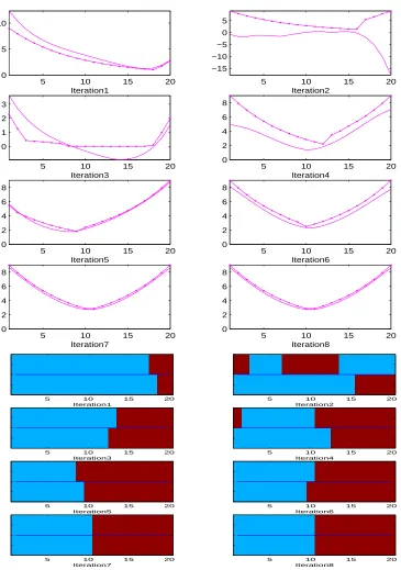
LSPI typically finds the optimal policy for this problem in 4 or 5 iterations. Samples for each run were collected in advance by choosing actions uniformly at random for about 25 (or more) steps and the same sample set was used throughout all LSPI iterations in the run. Figure 10 shows the iterations of one run of LSPI on a training set of 50 samples. States are shown on the horizontal axis and Q values on the vertical axis. The approximations are shown with solid lines, whereas the exact values are connected with dashed lines. The values for action L are marked with ◦ and for action R with ∗. LSPI finds the optimal policy by the 2nd iteration, but it does not terminate until the 4th iteration, at which point the successive parameters (3rd and 4th iterations) are approximately equal. Notice that the approximations capture the qualitative structure of the value function, although the quantitative error is fairly big. The state visitation distribution for this training set was (0.24, 0.14, 0.28, 0.34). Although it was not perfectly uniform, it was “flat” enough to prevent an extremely uneven allocation of approximation errors over the state-action space. LSPI was also tested on variants of the chain walk problem with more states and different reward schemes to better understand and illustrate its behavior. Figure 11 shows a run of LSPI on a 20-state chain with the same dynamics as above and a reward of +1 given only at the boundaries (states 1 and 20). The optimal policy in this case is to go left in states 1–10 and right in states 11–20. LSPI converged to the optimal policy after 8 iterations using a single set of samples collected from a single episodes in which actions were chosen uniformly at random for 5000 steps. A polynomial of degree 4 was used for approximating the value function for each of the two actions, giving a block of 5 basis functions per action,
1 2 3 4 −1
0 1 2 3
1st iteration: RRRR −> RLLL
1 2 3 4
0 1 2 3 4 5 6 7
2nd iteration: RLLL −> RRLL
1 2 3 4
0 2 4 6 8
3rd iteration: RRLL −> RRLL
1 2 3 4
0 2 4 6 8
4th iteration: RRLL −> RRLL
Figure 10: LSPI applied on the problematic MDP.
or a total of 10 basis functions. The initial policy was the policy that chooses left (L) in all states. LSPI eventually discovered the optimal policy, although in iteration 2 it found neither a good approximation to the value function nor an improved policy. This example illustrates the non-monotonic nature of policy improvement between iterations of LSPI due to value function approximation errors.
Figure 12 shows an example where LSPI fails to discover the optimal policy because of limited representational ability of the linear architecture. In this 50-state chain, reward is given only in states 10 and 41 and therefore due to the symmetry the optimal policy is to go right in states 1–9 and 26–41 and left in states 10–25 and 42–50. Again, a polynomial of degree 4 was used for each of the actions. Using a single training set of 10000 samples (all from a single “random walk” trajectory), LSPI converged after 6 iterations to a suboptimal policy that nevertheless resembles the optimal policy to a good extent. This failure can be explained as an inability of the polynomial approximator to capture the precise structure of the underlying value function. This behavior was fairly consistent with different sample sets and/or increased sample size. In all runs, LSPI converged in less than 10 iterations to fairly good, but not optimal, policies.
5 10 15 20 0
5 10
Iteration1
5 10 15 20
−15 −10 −5 0 5 Iteration2
5 10 15 20
0 1 2 3
Iteration3
5 10 15 20
0 2 4 6 8 Iteration4
5 10 15 20
0 2 4 6 8 Iteration5
5 10 15 20
0 2 4 6 8 Iteration6
5 10 15 20
0 2 4 6 8 Iteration7
5 10 15 20
0 2 4 6 8 Iteration8 Iteration1
5 10 15 20
Iteration2
5 10 15 20
Iteration3
5 10 15 20
Iteration4
5 10 15 20
Iteration5
5 10 15 20
Iteration6
5 10 15 20
Iteration7
5 10 15 20
Iteration8
5 10 15 20
5 10 15 20 25 30 35 40 45 50 −3
−2 −1 0 1
Iteration1
5 10 15 20 25 30 35 40 45 50 0
0.5 1 1.5
Iteration2
5 10 15 20 25 30 35 40 45 50 0
1 2
Iteration3
5 10 15 20 25 30 35 40 45 50 0
0.5 1 1.5
Iteration4
5 10 15 20 25 30 35 40 45 50 0
0.5 1 1.5
Iteration5
5 10 15 20 25 30 35 40 45 50 0
0.5 1 1.5
Iteration6
Iteration1
10 20 30 40 50
Iteration2
10 20 30 40 50
Iteration3
10 20 30 40 50
Iteration4
10 20 30 40 50
Iteration5
10 20 30 40 50
Iteration6
10 20 30 40 50
5 10 15 20 25 30 35 40 45 50 0
0.5 1 1.5
Iteration1
5 10 15 20 25 30 35 40 45 50 −0.5
0 0.5 1 1.5
Iteration2
5 10 15 20 25 30 35 40 45 50 0
2 4
Iteration3
5 10 15 20 25 30 35 40 45 50 0
2 4
Iteration4
5 10 15 20 25 30 35 40 45 50 0
2 4
Iteration5
5 10 15 20 25 30 35 40 45 50 0
2 4
Iteration6
5 10 15 20 25 30 35 40 45 50 0
2 4
Iteration7
Iteration1
10 20 30 40 50
Iteration2
10 20 30 40 50
Iteration3
10 20 30 40 50
Iteration4
10 20 30 40 50
Iteration5
10 20 30 40 50
Iteration6
10 20 30 40 50
Iteration7
10 20 30 40 50
LSPI makes a call to LSTDQ, which learns the least-squares fixed-point approximation to the state-action value function given a set of samples. Alternatively, LSPI could call some other learning procedure, similar to LSTDQ, which instead would learn the Bellman residual minimizing approximation. For this modified version of LSTDQ, the update equations for learning would be:
e
A(t+1)=Ae(t)+φ(st, at)−γφ s00t, π(s00t)
φ(st, at)−γφ s0t, π(s0t) |
,
eb(t+1)=eb(t)+φ(s
t, at)−γφ s00t, π(s00t)
rt .
For comparison purposes, this modified version of LSPI was applied to the 50-state problem discussed above (same parameters, same number and kind of training samples).11 Figure 14 and Figure 15 show the results for the polynomial and the radial basis function approximators respectively. In both cases, the approximations of the value function seem to be “close” to the true value functions. However, in both cases, this modified version of LSPI exhibits a non-convergent behavior (only the first 8 iterations are shown). With either approximator, the iteration initially proceeds toward better policies, but fails to discover the optimal policy. The resulting policies are somewhat better with the radial basis function approximator, but in either case they are worse than the ones found by LSPI with the least-squares fixed-point approximation. This behavior of LSPI combined with the Bellman residual minimizing approximation was fairly consistent and did not improve with increased sample size.
It is not clear why the least-squares fixed-point solution works better than the Bell-man residual minimizing solution. We conjecture that the fixed-point solution preserves the “shape” of the value function (the relative magnitude between values) to some extent rather than trying to fit the absolute values. In return, the improved policy from the ap-proximate value function is “closer” to the improved policy from the corresponding exact value function, and therefore policy iteration is guided to a direction of improvement. Of course, this point needs further investigation.
9.2 Inverted Pendulum
Theinverted pendulumproblem requires balancing a pendulum of unknown length and mass at the upright position by applying forces to the cart it is attached to. Three actions are allowed: left force LF (−50 Newtons), right force RF (+50 Newtons), or no force NF (0 Newtons). All three actions are noisy; uniform noise in [−10,10] is added to the chosen action. The state space of the problem is continuous and consists of the vertical angle θ
and the angular velocity ˙θof the pendulum. The transitions are governed by the nonlinear dynamics of the system (Wang et al., 1996) and depend on the current state and the current (noisy) control u:
¨
θ= gsin(θ)−αml( ˙θ)
2sin(2θ)/2−αcos(θ)u 4l/3−αmlcos2(θ) ,
11. To generate the necessary “doubled” samples, for each sample (s, a, r, s0) in the original set, another sample (s, a, r0
, s00
5 10 15 20 25 30 35 40 45 50 0
0.5 1 1.5
Iteration1
5 10 15 20 25 30 35 40 45 50 0
0.5 1 1.5
Iteration2
5 10 15 20 25 30 35 40 45 50 0
0.5 1 1.5
Iteration3
5 10 15 20 25 30 35 40 45 50 0
2 4
Iteration4
5 10 15 20 25 30 35 40 45 50 0
1 2
Iteration5
5 10 15 20 25 30 35 40 45 50 0
2 4
Iteration6
5 10 15 20 25 30 35 40 45 50 0
0.5 1 1.5
Iteration7
5 10 15 20 25 30 35 40 45 50 0
2 4
Iteration8
Iteration1
10 20 30 40 50
Iteration2
10 20 30 40 50
Iteration3
10 20 30 40 50
Iteration4
10 20 30 40 50
Iteration5
10 20 30 40 50
Iteration6
10 20 30 40 50
Iteration7
10 20 30 40 50
Iteration8
10 20 30 40 50