PhD Dissertation
International Doctorate School in Information and Communication Technologies
DISI - University of Trento
A Reactive Search Optimization approach
to interactive decision making
Paolo Campigotto
Advisor:
Prof. Roberto Battiti
Universit`a degli Studi di Trento
Abstract
Reactive Search Optimization (RSO) advocates the integration of learning techniques into search heuristics for solving complex optimization problems. In the last few years, RSO has been mostly employed in self-adapting a local search method in a manner depending on the previous history of the search. The learning signals consisted of data about the structural characteristics of the instance collected while the algorithm is running. For example, data about sizes of basins of attraction, entrapment of trajectories, repetitions of previously visited configurations. In this context, the algorithm learns by interacting from a previously unknown environment given by an existing (and fixed) problem definition.
This thesis considers a second interesting online learning loop, where the source of learning signals is the decision maker, who is fine-tuning her preferences (formalized as an utility function) based on a learning process triggered by the presentation of tentative solutions. The objective function and, more in general, the problem definition is not fully stated at the begin-ning and needs to be refined during the search for a satisfying solution. In practice, this lack of complete knowledge may occur for different reasons: insufficient or costly knowledge elicitation, soft constraints which are in the mind of the decision maker, revision of preferences after becoming aware of some possible solutions, etc.
paradigm of Interactive Decision Making (IDM). In particular, it consid-ers interactive optimization from a machine learning pconsid-erspective, where IDM is seen as a joint learning process involving the optimization com-ponent and the DM herself. During the interactive process, on one hand, the decision maker improves her knowledge about the problem in question and, on the other hand, the preference model learnt by the optimization component evolves in response to the additional information provided by the user. We believe that understanding the interplay between these two learning processes is essential to improve the design of interactive decision making systems. This thesis goes in this direction, 1) by considering a final user that may change her preferences as a result of the deeper knowledge of the problem and that may occasionally provide inconsistent feedback dur-ing the interactive process, 2) by introducdur-ing a couple of IDM techniques that can learn an arbitrary preference model in these changing and noisy conditions. The investigation is performed within two different problems settings, the traditional multi-objective optimization and a constraint-based formulation for the DM preferences.
and by the suitable trade-off among diversification and intensification of the search during the optimization stage.
Keywords
Contents
1 Introduction 3
1.1 Multi-objective optimization formulation . . . 5
1.2 Motivation of the thesis . . . 6
1.2.1 Preferences as soft constraints . . . 8
1.3 Contribution of the thesis . . . 10
1.3.1 Contribution in interactive multi-objective optimiza-tion . . . 11
1.3.2 Constraint-based formulation . . . 13
1.4 Outline of the thesis . . . 16
2 Handling preference drift in interactive decision making 17 2.1 Introduction . . . 18
2.2 Interactive decision making techniques . . . 20
2.3 The BC-EMO algorithm . . . 22
2.4 Handling preference drift with BC-EMO . . . 25
2.5 Experimental results . . . 27
2.6 Conclusion . . . 32
3 Active Learning of Combinatorial Features for Interactive Optimization 35 3.1 Introduction . . . 36
3.3 Satisfiability Modulo Theory . . . 42
3.3.1 Satisfiability Modulo Theory solvers . . . 43
3.3.2 Weighted MAX-SMT . . . 45
3.4 Related works . . . 46
3.4.1 Constraint programming approaches for preference elicitation . . . 48
3.5 Experimental results . . . 52
3.5.1 Weighted MAX-SAT . . . 52
3.5.2 Weighted MAX-SMT . . . 56
3.6 Discussion . . . 65
4 Conclusions and perspectives 69
Bibliography 73
A Expressing bipolar preferences within the soft constraints
formalism 81
Acknowledgements
Chapter 1
Introduction
In many decision making problems, the crucial issue is not that of deliv-ering a single solution, but that of critically analyzing a mass of tentative solutions, which can easily grow up to thousands or millions, to identify the solution preferred by the final user. Delivering to the decision maker (DM) the entire set of the tentative solutions so that the user can pick her most preferred solution is impractical, due to the prohibitive effort required to the DM.
In principle, this laborious selection among the large set of candidate solutions could be avoided by including in the initial formulation of the problem the specification of the utility criterion of the DM. However, re-quiring a human DM to pre-specify her preferences, without seeing any actual optimization result, is extremely difficult. In typical decision mak-ing problems the preferences of the DM cannot be fully defined at the beginning and needs to be learnt and refined during the search for a sat-isfying solution. This lack of complete knowledge can occur for different reasons: insufficient or costly knowledge elicitation, soft constraints which are in the mind of the decision maker, revision of the preferences after becoming aware of some possible solutions, etc.
CHAPTER 1. INTRODUCTION
by keeping the user in the loop of the optimization process. They use pref-erence information from the decision maker during the optimization task to guide the search towards her favourite solution. This thesis introduces two new interactive decision making techniques. With the extent of identi-fying the favourite solution of the decision maker, they learn and optimize an approximation of the preference model of the final user.
One technique is developed within the context of the traditional multi-objective optimization problem, where the user searches for her favourite solution within the Pareto-optimal set. Our approach considers the limited and bounded rationality of the humans when making decisions: it accounts for noisy and inconsistent feedback from the user and can handle a DM preference model that changes over time. The incomplete knowledge about the problem to be solved is formalized by assuming the knowledge of a set of desirable objectives, and ignorance of their detailed combination. To the best of our knowledge, in the context of multi-objective optimization no interactive decision making technique has been explicitly designed to handle a preference model that evolves over time. This work aims at cover-ing this gap, by introduccover-ing also a representative multi-objective problem with evolving user preferences.
util-CHAPTER 1. INTRODUCTION1.1. MULTI-OBJECTIVE OPTIMIZATION FORMULATION
ity function modeling the quality of the candidate solutions and uses it to generate novel candidates for the following refinement. The learning stage exploits the sparsity-inducing property of 1-norm regularization to learn a combinatorial function from the power set of all possible conjunctions up to a certain degree. The optimization stage uses a satisfiability modulo theories solver, which enables the definition of a general approach for a large class of optimization problems.
1.1
Multi-objective optimization formulation
Modeling real world problems often generates optimization tasks involving multiple and conflicting objectives. Because the objectives are in conflict, a solution simultaneously optimizing all of them does not exist. The terms
multiple criteria decision making or multi-objective optimization refers to solving these problems. A multi-objective optimization problem (MOOP) can be stated as:
minimize f(x) ={f1(x), . . . , fm(x)} (1.1)
subject to x∈ Ω
where x ∈ Rn is a vector of n decision variables; Ω ⊂ Rn is the feasible region and is typically specified as a set of constraints on the decision
variables; f : Ω → Rm is a vector of m objective functions which need
to be jointly minimized. Objective vectors are images of decision vectors and can be written as z = f(x) = {f1(x), . . . , fm(x)}. Problem 1.1 is
1.2. MOTIVATION OF THE THESIS CHAPTER 1. INTRODUCTION
to dominate z′, denoted as z ≻ z′, if zk ≤ z′k for all k and there exist at
least one h such that zh < zh′. A point ˆx is Pareto-optimal if there is no
other x ∈ Ω such that f(x) dominates f(ˆx). The set of Pareto-optimal points1 is called Pareto set (PS). The corresponding set of Pareto-optimal objective vectors is called Pareto front (PF).
1.2
Motivation of the thesis
The centrality of the decision maker is widely recognized in the multiple cri-teria decision making community. However, in the experiments considered in IDM literature the user preferences are usually formalized into a math-ematical model, with the extent of representing the qualitative notion of preference as a quantitative function, while retaining the Pareto-optimality properties. This mathematical model emulates the decision maker in the interactive optimization process. The preference model is usually repre-sented by the linear combination of the objectives or it is expressed as a function of the distance from the ideal point. In the first case, the model is formalized into a function U(z) as follows:
U(z) =
m
X
k=1
wkzk (1.2)
where the (positive) weights encode the relative importance of the different objectives. In the second case, the utility function is defined by a weighted-Lp metric of the following form:
U(z) =−
m
X
k=1
wk|zk∗ −zk|p
!1/p
(1.3)
1In the multi-objective optimization literature, these trade-off solutions are known by means of
CHAPTER 1. INTRODUCTION 1.2. MOTIVATION OF THE THESIS
in which z∗ is a reference ideal objective vector obtained by separately maximizing each objective function subject to the feasible region, i.e.,zk∗ = maxx∈Ωfk(x).
The utility functions in Eq. 1.2 and 1.3 are used to simulate the feedback of a real user during the interactive process. That is, the preference of the user for the solution z′ is expressed by the value U(z′). This approach has several limitations:
1. the linear weighting scheme in Eq. 1.2 cannot model the typical human decision making process occurring in many real life situa-tions. When a strong non-linear relation correlates the different ob-jectives, the most intuitive approach of giving highest weight to the most important criterion can lead to completely unsatisfactory solu-tions [41, 45]. In many decision making situasolu-tions, assuming that satisfaction increases linearly with the decrease of the objective func-tions is inappropriate.
Even the generalization in Eq. 1.3 of the linear utility function can-not model the nonlinear preference of “compromise” solutions, which characterizes many human decision activities [4];
2. an error-free preference structure of the DM is assumed. However, im-precisions and contradictions characterize most human decision pro-cesses. As result, uncertain and inconsistent feedback is often observed in real decision making problems;
1.2. MOTIVATION OF THE THESIS CHAPTER 1. INTRODUCTION
aware of “what is possible”. Confronted with this new knowledge, her preferences may evolve over time. Typical scenarios involve a DM introducing new objectives in her preference model during the search, changing the relations between the different objectives or adjusting her preference model according to the observed limitations of the feasible set. As a results, her judgment changes over time.
According to [25], the number of real world applications of the optimization techniques developed by the multi-criteria decision making community is modest. The reason for this failure is the “high complexity of the methods as perceived by real decision makers” [25]. As matter of fact, the typical decision maker is not necessarily an expert in algorithmic and mathemati-cal details, but she is a user who needs a fast and simple way of navigating among the set of the Pareto-optimal solutions, guided by her preferences. These observations motivate the development of a robust preference elicita-tion phase in IDM techniques, enabling the user to express her preferences in a simple way, to change them over time and accounting for inconsistent feedback from the DM.
1.2.1 Preferences as soft constraints
The importance of learning the preference of the DM is not limited to the multi-objective optimization research community. In the last few years, the preference elicitation problem has been investigated in the context of differ-ent disciplines, including machine learning and constraint programming. In the machine learning (ML) community, the task of learning and predicting
preferences in an automatic way is known as preference learning [20]. As
CHAPTER 1. INTRODUCTION 1.2. MOTIVATION OF THE THESIS
constraint optimization problems where the data are not completely known before the solving process starts. In soft constraints, a generalization of hard constraints, each assignment to the variables of the constraint is as-sociated to a preference value taken from a preference set. The preference value represents the level of desirability of the assignment. The desirability of a complete assignment is computed by applying a combination operator to the local preference values. Thus, a set of soft constraints generates an order (partial or total) over the complete assignments of the variables of the problem. Given two solutions of the problem, the preferred one is selected by computing their preference levels and by comparing them in the preference order. The work in [21] introduces an elicitation strategy for soft constraint problems with missing preferences, to find the solution preferred by the decision maker asking the final user to reveal as few pref-erences as possible. Soft constraints are modeled by a general framework that can unify previous extensions of the constraint satisfaction formalism (e.g., weighted or fuzzy constraint satisfaction problems). The optimality of the solutions produced is guaranteed and the empirical studies in [21] show that on fuzzy constraint satisfaction problems with missing prefer-ences the algorithm can also provide a solution at any point in time, whose quality increases with the computation time (anytime property).
However, the work in in [21] has several limitations and open issues:
• it does not consider the inconsistent and imprecise preference infor-mation from the DM characterizing many human decision processes;
• it assumes initial complete knowledge of both the decisional features of the DM and their detailed combination (represented in terms of soft constraints). The elicitation process focuses exclusively on assessing the weights of the soft constraints;
1.3. CONTRIBUTION OF THE THESIS CHAPTER 1. INTRODUCTION
assignments to the variables of a specific constraint. However, asking to the final user precise scores is in many cases inappropriate or even impossible. Most of the users are typically more confident in compar-ing solutions, providcompar-ing qualitative judgments like “I prefer solution A to solution B”, rather than in specifying how much they prefer A over B;
• it models just negative preferences, i.e., the final user can express just different degrees of unsatisfaction for the solutions. In many real life problems, the interaction with the final users is naturally modeled by specifying what she likes and what she dislikes, reflecting the typi-cal human behavior, where the degree of preference for a solution is defined by comparing its advantages with its disadvantages;
• it combines branch and bound search with preference elicitation, the adoption of local search algorithms is a matter of current research, as pointed out by the authors themselves.
In this thesis, we introduce a technique that can solve the above issues, testing its performance over a couple of realistic decision problems.
1.3
Contribution of the thesis
This thesis tackles the problem of learning the user preferences in the context of interactive decision making. In particular, we formalize the preference learning problem within two settings:
1. the traditional multi-objective optimization formulation;
2. a constraint-based formulation modeling the DM preferences.
CHAPTER 1. INTRODUCTION 1.3. CONTRIBUTION OF THE THESIS
contradictory and inconsistent feedback from the decision maker as well as a dynamic preference model of the final user.
1.3.1 Contribution in interactive multi-objective optimization
Concerning the traditional MOOP, the contribution of this thesis consists of a new technique that can handle unforeseen changes in the preferences of the decision maker. Real world optimization tasks are often characterized by noisy and changing conditions. The problem of learning in changing conditions is known in the machine learning community as learning under
concept drift [39]. The problem has received increasing attention in past few years, and a number of solutions have been proposed to tackle it. For a review of the recent approaches in this area, see [51]. In this thesis we consider concept drift in the specific setting of interactive optimization. We call preference drift the tendency of the decision maker to change her preferences during the interactive optimization stage. To the best of our knowledge, the current IMO techniques usually consider a static prefer-ence model for the DM: no IMO technique has been explicitly designed to handle preference drift. Among the plethora of IMO algorithms, ref-erence point methods [29, 30], which iteratively minimize the distance to ideal reference points provided by the DM, could in principle naturally handle preference drifts. However, the cognitive demands required to the DM can easily become prohibitive, especially when dealing with non-linear preference models and an increasing number of objectives.
1.3. CONTRIBUTION OF THE THESIS CHAPTER 1. INTRODUCTION
algorithm [4] overcomes these limitations. BC-EMO is a genetic algorithm that learns the preference information of the decision maker (formalized as a value function) by the feedback received when the DM evaluates ten-tative solutions. Based on this feedback, the predicted value function is refined, and it is used to modify the fitness measure of the genetic al-gorithm. Fast convergence of the algorithm to the desired solution was shown [4] on both combinatorial and continuous problems with linear and non-linear value functions. The learning stage is based on a support vector ranking algorithm which provides robustness to inaccurate and contradic-tory DM feedback [8]. We thus selected BC-EMO as a natural candidate to be extended for managing preference drift [9].
The extension of BC-EMO for preference drift recovery is based on the approach of instance weighting [27], a popular strategy in the concept drift literature. The instance weighting technique consists of reweighting the examples according to their predicted relevance for the current concept. We include this reweighting scheme in the learning component of the BC-EMO algorithm, a change detection monitor is responsible for activating the mechanism. In order to deal with concept drift in the specific setting of interactive optimization, we also introduce a diversification strategy aimed at escaping from minima which could become suboptimal for the changed utility function of the DM.
CHAPTER 1. INTRODUCTION 1.3. CONTRIBUTION OF THE THESIS
into the definition of benchmark problems characterized by:
1. highly complex Pareto front, including concave, convex and discon-nected regions;
2. arbitrary DM preference model;
3. uncertain, inconsistent and contradictory feedback from the final user;
4. unforeseen changes in the preferences of the decision maker.
Uncertain preference information is modeled by considering occasional inattention of the DM or her embarrassment when required to compare too similar solutions. Evaluating the ability of the proposed preference model to simulate the human decision process is outside the scope of this work. The generation of benchmark problems with the above characteris-tics provides test cases for the extended version of BC-EMO, and, more in general, may help to identify the MOO algorithms that are more promising for future testing on real-life scenarios.
1.3.2 Constraint-based formulation
In many real-life problems, preferences can be naturally expressed as soft constraints. Given the set of soft constraints, the aim consists of finding a solution optimizing them. This means that there is an utility function measuring the quality of the candidate solutions in terms of preferences.
1.3. CONTRIBUTION OF THE THESIS CHAPTER 1. INTRODUCTION
the constraints, with the weights defining the relative importance of the constraints.
In the setting we consider here the combinatorial utility function ex-pressing the DM preference model is the weighted combination of Boolean terms. However, it is unknown and has to be jointly and interactively learned during the optimization process. Note that the optimal utility
function is complex enough to prevent exhaustive enumeration of possible
solutions.
Our method consists of an iterative procedure alternating a search phase with a model refinement phase. At each step, the current approximation of the utility function is used to guide the search for optimal configurations; preference information is required for a subset of the recovered candidates, and the utility model is refined according to the feedback received. A set of randomly generated examples is employed to initialize the utility model at the first iteration.
CHAPTER 1. INTRODUCTION 1.3. CONTRIBUTION OF THE THESIS
a satisfying assignment as in SMT, the target is a satisfying assignment that minimizes a given cost function. Optimization modulo theories is a very recent research field; this is the first work combining learning, inter-active optimization and SMT. Therefore, to test our IDM technique we encoded different optimization tasks as weighted MAX-SMT optimization problems.
Considering our critique to the soft constraint-based approach in [21], our technique offers the following advantages:
• it does not assume to know in advance the decisional features of the user and their detailed combination. It can select the variables of the learning problem from a set of “catalog” features;
• it can handle noisy and inconsistent feedback from the user;
• it may adapt to both qualitative and quantitative evaluations from the DM, by asking the comparison of solutions rather than the assignment of preference degrees in terms of scores from a predefined range;
• in the case of quantitative evaluations from the DM, it allows the
user to state both negative or positive judgments for the provided solutions, including the possibility to express “indifference”;
• both complete and local search techniques may be adopted to optimize the learnt preference model.
1.4. OUTLINE OF THE THESIS CHAPTER 1. INTRODUCTION
1.4
Outline of the thesis
Chapter 2
Handling preference drift in
interactive decision making
2.1. INTRODUCTION
CHAPTER 2. HANDLING PREFERENCE DRIFT IN INTERACTIVE DECISION MAKING
for a representative preference drift scenario are presented.
2.1
Introduction
Modeling real-world problems often generates optimization tasks involving multiple and conflicting objectives. Because the objectives are in conflict, a solution simultaneously optimizing all of them does not exist. The typical approach to multi-objective optimization problems (MOOPs) consists of searching for a set of trade-off solutions, called Pareto-optimal set, for which any single objective cannot be improved without compromising at least one of the other objectives.
Usually, the size of the Pareto-optimal set is large or infinite and the decision maker (DM) cannot tackle the overflow of information generated when analyzing it entirely. In this scenario, interactive decision making (IDM) techniques come to the rescue. They assume that the optimization expert (or the optimization software) cooperates with the DM. Through the interaction, the search process can be directed towards the DM pre-ferred Pareto-optimal solutions and only a fraction of the Pareto-optimal set needs to be generated.
CHAPTER 2. HANDLING PREFERENCE DRIFT IN INTERACTIVE DECISION
MAKING 2.1. INTRODUCTION
alert the optimization component. From a learning perspective, interactive multi-objective optimization should thus be seen as a joint learning process involving the model and the DM herself [5].
In the machine learning (ML) community, the problem of learning in
these changing conditions is known as learning under concept drift [39].
The work in [51] reviews the recent approaches for concept drift recovery. In this thesis we consider preference drift, the tendency of the decision maker to change her preferences during the interactive optimization stage. To the best of our knowledge, no IDM technique has been explicitly de-signed to handle preference drift. Among the plethora of IDM algorithms, reference point methods [29, 30], which iteratively minimize the distance to ideal reference points provided by the DM, could in principle naturally handle preference drifts. However, the cognitive effort of the DM can eas-ily become prohibitive, especially when dealing with non-linear preference models and an increasing number of objective.
Different IDM approaches [43, 44, 23] employ machine learning tech-niques to learn the user preferences and can be easily adapted to tackle preference drifts. However, these approaches cannot guarantee the gener-ation of Pareto optimal solutions or assume a linear set of weights, one for each objective. A recent genetic technique, the Brain-Computer Evolu-tionary Multi-Objective Optimization (BC-EMO) algorithm [4], overcomes these limitations.
2.2. INTERACTIVE DECISION MAKING TECHNIQUES
CHAPTER 2. HANDLING PREFERENCE DRIFT IN INTERACTIVE DECISION MAKING
by the adoption of a support vector ranking technique in the learning stage of BC-EMO. We thus selected BC-EMO as a natural candidate to be extended for managing preference drift.
The extension of BC-EMO for preference drift recovery exploits the instance weighting scheme [27] from the concept drift literature, which reweights the examples according to their predicted relevance for the cur-rent concept. The activation of the reweighting mechanism is triggered by a change detection monitor. Furthermore, in order to deal with concept drift in the specific setting of interactive optimization, a diversification strategy aimed at escaping from minima which could become suboptimal for the changed preference of the DM is also introduced.
The remainder of the chapter is organized as follows. Section 2.2 intro-duces IDM and discusses the limitations of current techniques in regard to preference drift handling. Section 2.3 briefly reviews the BC-EMO al-gorithm, while Section 2.4 extends it to automatically handle preference drift. An experimental evaluation of the proposed extension is reported in Section 2.5. Section 2.6 draws some conclusions and proposes possible directions for future research.
2.2
Interactive decision making techniques
Several IDM approaches have been developed to aid the DM in identify-ing her preferred solution [31], includidentify-ing evolutionary multi-objective al-gorithms (see for example [15] and contained references). IDM procedures exploit the preference feedback from the DM to refine a preference model, usually expressed as a value function.
CHAPTER 2. HANDLING PREFERENCE DRIFT IN INTERACTIVE DECISION MAKING 2.2. INTERACTIVE DECISION MAKING TECHNIQUES
reference point specifies the desirable values of the objectives and it is usually provided by the DM. The distance from the reference point has a
preferential meaning: the tentative solution x∗ ∈ Ω showed to the DM is
the solution minimizing the deviation from the reference point. In detail, the solution x∗ is obtained by solving the following program:
x∗ = min max
k=1...m[wk(fk(x)−z¯k)] (2.1)
subject to x∈ Ω
with weight wk > 0, k = 1. . . m. The achievement scalarizing function to
minimize in Eq. 2.1 is the weighted Tchebychev distance from the reference point. The DM can express her bias for the k-th objective by assigning a value to weight wk. After the DM has specified her desirable solution as
a reference point, she can see what was feasible (the solution x∗) and in case provide a new reference point. Let us emphasize the rationale of this approach:
1. the location of the reference point causes the procedure to focus on a certain region in the Pareto front;
2. a local approximation of the preference model is expressed by the dis-tance function from the reference point. Using the weighted Tcheby-chev distance metric, every solution of the Pareto front can be ob-tained by altering the reference point only [48].
Many refinements and extensions of this approach exist [30]. They con-sider different ways of interaction with the DM (e.g., by showing a set of solution in the neighborhood ofx∗) and different refinements of the achieve-ment scalarizing function, designed to obtain Pareto-optimal solutions with particular properties.
2.3. THE BC-EMO ALGORITHM
CHAPTER 2. HANDLING PREFERENCE DRIFT IN INTERACTIVE DECISION MAKING
in her preferences. However, the effort of the decision maker to modify the reference point when her preference model includes non-linear relations be-tween the objectives may be prohibitive. The cognitive demands become unrealistic when the dimensionality of the problem increases, providing a large set of candidate directions to shift the reference point.
In the past, a number of works [43, 44, 23] introduced ML-based ap-proaches to learn the user preferences in an interactive fashion. However, they have several limitations [4]. The approach in [43] does not guarantee the generation of Pareto optimal solutions, while the strategies developed in [44, 23] generate a linear local approximation of the user preferences and do not use directly the learned preference model to drive the search. Furthermore, in all these works the feedback from the DM is expressed in terms of quantitative scores.
The BC-EMO algorithm [4] overcomes these limitations, by learning the preference model with pairwise preference supervision, a much more affordable task for the DM, and by directly using the preference model to drive the search over the Pareto front. The algorithm does not make any assumption about the preference structure of the DM, possibly accounting for highly non-linear relations between the different objectives. This work extends BC-EMO to handle preference drift.
2.3
The BC-EMO algorithm
CHAPTER 2. HANDLING PREFERENCE DRIFT IN INTERACTIVE DECISION
MAKING 2.3. THE BC-EMO ALGORITHM
Algorithm 1Training procedure at the generic i-th EMO iteration
1: procedure Train(Pi, Ui−1, exa)
2: Ptr ← PrefOrder(Pi,Ui−1,exa)
3: obtain pairwise preferences for Ptr from the DM
4: sort Ptr according to user preferences and add it to training instances
5: Choose best kernelK and regularization C by k-fold cross validation 6: Ui ←function trained on full training set with K and C
7: resi ←k-fold cv estimate of function performance
8: return Ui, resi
9: end procedure
ranking constraints for the learning algorithm. No specific assumptions are made about the form of the DM value function: BC-EMO has a tuning phase selecting the most appropriate kernel (i.e., similarity measure) in or-der to best approximate the targets, allowing it to learn an arbitrary value function provided enough data are available. Furthermore, support vector ranking allows to effectively deal with noisy training observations thanks to a regularization parameter C trading-off data fitting with complexity of the learned model.
The learned value function is used to rank the current population during the selection phase of the BC-EMO algorithm, where a sub-population is selected for reproduction on the basis of fitness (i.e., quality of the solu-tions). In particular, the BC-EMO selection procedure, which we will refer
to as PrefOrder, consists of:
1. collecting the subset of non-dominated individuals in the population;
2. sorting them according to the learned value function;
3. appending to the sorted set the result of repeating the procedure on the remaining dominated individuals, until the desired number of in-dividuals is reached.
2.3. THE BC-EMO ALGORITHM
CHAPTER 2. HANDLING PREFERENCE DRIFT IN INTERACTIVE DECISION MAKING
form of the learned value function. Any evolutionary multi-objective algo-rithm (EMOA) that needs comparisons between candidate individuals can be equipped with the BC-EMO selection procedure (replacing or integrat-ing the original selection procedure). Algorithm 1 describes the procedure of the generic i-th training iteration, in which: 1) the exa best individuals
from the current population Pi are selected according toPrefOrder with
current value function Ui−1; 2) DM feedback is collected for these exam-ples; 3) parameter selection, training and evaluation are conducted on the
training data enriched with Ptr. This procedure will be modified in the
next section in order to account for preference drifts. The overall BC-EMO approach consists of three steps:
1. initial search phase: the plain EMOA selected is run for a given num-ber of generations and produces a final population P1;
2. training phase: using P1 as initial population, a specific number of training iterations are executed to learn the value function V by in-teracting with the DM. The final population obtained (P2) is collected;
3. final search phase: the selected EMOA equipped with the BC-EMO selection procedure is run for a given number of generations, using P2 as initial population and producing the final ordered population.
Each training iteration alternates a refinement phase, where the DM is queried for feedback on candidate solutions and the value function is up-dated according to such feedback, with a search phase, where the EMOA equipped with the BC-EMO selection procedure is run for a given number of iterations. The training phase is executed until the maximum number of training iterations or the desired accuracy level are reached.
CHAPTER 2. HANDLING PREFERENCE DRIFT IN INTERACTIVE DECISION
MAKING 2.4. HANDLING PREFERENCE DRIFT WITH BC-EMO
(exa), the number of generations before the first training iteration (gen1) and between two successive training iterations (gens). Algorithm 2
con-tains the pseudocode of the BC-EMO approach applied on top of a generic EMO algorithm. Further details on the algorithm can be found in [4].
Algorithm 2The BC-EMO algorithm
1: procedure BC-EMO(maxit, exa, gen
1, gens)
2: res←0, it←0, U ←Rand
3: run the EMOA forgen1 generations
4: collect last population P
5: while it≤maxit do
6: U, res←Train(P, U,exa)
7: run the EMOA for gens generations guided PrefOrder with U
8: collect last population P
9: end while
10: run the EMOA for the remaining generations guided PrefOrderwith U
11: return the final populationP
12: end procedure
2.4
Handling preference drift with BC-EMO
The effect of preference drift is a decrease of the accuracy of the learnt model over time. In the original version of BC-EMO, training data arrives in batches over time and the model is re-trained every gens generations,
when a new batch of training examples is available. The extension to handle preference drift consists of a mechanism for drift detection and of a reweighting of the past training examples inversely proportional to the observed decrease in the performance accuracy.
2.4. HANDLING PREFERENCE DRIFT WITH BC-EMO
CHAPTER 2. HANDLING PREFERENCE DRIFT IN INTERACTIVE DECISION MAKING
Ui−1 the new batch of observable data and the current model at the generic i-th training iteration, respectively. The performance of the current model is the prediction accuracy 0 ≤ resi−1 ≤ 1 over batchbi−1. Furthermore, let 0 ≤ res′i−1 ≤ 1 the prediction accuracy of the current model over batch bi.
If the difference between resi−1 and res′i−1 is bigger than a fixed threshold td, with td > 0, a drift in the preferences of the decision maker is assumed.
In this case, the cost of the training examples collected so far (i.e., the training examples of batches b1, b2, . . . bi−1) is decreased as a function of the value resi−1−res′i−1. In detail, the cost is updated by a multiplicative factor d = c(resi−1 −res′i−1), where the function c is defined as follows:
c(x) =
1 if x ≤ td
1−x if td < x < 0.5
0 if x ≥ 0.5
(2.2)
Let us comment. If the value resi−1 −res′i−1 is bigger than the threshold and smaller than 0.5, the cost of the training examples is decreased by the normalized value of the difference res′i−1 − resi−1. When the decrease of the performance accuracy over the last batch of observable data is bigger than value 0.5, the training examples of the previous batches are discarded (i.e., their cost becomes zero). The rationale for this choice is that a large decrease in the accuracy of the learnt model is seen as symptom of a radical change in the preferences of the DM, outdating training examples collected in previous iterations.
If a drift in the preferences of the user has been detected, the model selection phase is executed using only the data in the i-th batch rather than using all the collected examples, as in the original version of BC-EMO (algorithm 1, line 6). Furthermore, the genetic population of the EMOA is reinitialized.
CHAPTER 2. HANDLING PREFERENCE DRIFT IN INTERACTIVE DECISION
MAKING 2.5. EXPERIMENTAL RESULTS
resi is smaller than threshold tr, the selected model is discarded as it does
not satisfy the minimal performance requirement, and all training examples of of batches b1. . . bi−1 are discarded as well. The plain EMOA underlying BC-EMO will then be executed starting with a random population, until the next training iteration is reached. The rationale for this choice is the assumption that the poor performance of the selected model is caused by the collected training examples, localized in a region of the Pareto front that does not provide informative examples to learn the drift of the user preferences. The plain EMOA algorithm is executed to generate a population representing the whole Pareto front (without considering the preferences of the decision maker), in order to create more informative training examples at the next training iteration.
Algorithm 3 describes the modification of the training procedure at the generic i-th training iteration of BC-EMO to handle preference drift.
2.5
Experimental results
The experimental evaluation is focused on demonstrating the effectiveness of the extension of BC-EMO to handle decision maker preference drift for a selected case study. Given this focus, we did not attempt to fine-tune non-critical parameters which were fixed for the experiment.
Following [4], BC-EMO has been applied on top of NSGA-II [16] EMOA. We chose a population size of 100, 2000 generations, probability of crossover equal to one and probability of mutation equal to the inverse of the num-ber of decision variables. Concerning the learning task of BC-EMO, the number of initial generations (gen1) was set to 200, while the number of generations between two training iterations (gens) was set to 100. Both
2.5. EXPERIMENTAL RESULTS
CHAPTER 2. HANDLING PREFERENCE DRIFT IN INTERACTIVE DECISION MAKING
Algorithm 3 Training procedure to handle preference drift
1: procedure Train(Pi, Ui−1, exa, resi−1,td, tr)
2: Ptr ← PrefOrder(Pi,Ui−1,exa)
3: obtain pairwise preferences for Ptr from the DM
4: bi ← sort Ptr according to user preferences
5: Addbi to training instances
6: res′
i−1 ← test Ui−1 using bi
7: if resi−1−res′i−1 > td then
8: Decrease costs of examples in b1. . . bi−1 according to (2.2) usingtd
9: Re-initialize Pi randomly
10: end if
11: Choose best kernelK and regularization C by k-fold cross validation 12: resi ←k-fold cv estimate of function performance
13: if resi ≥tr then
14: Ui ← function trained on full training set with K and C
15: else
16: resi ←0,Ui ←Rand
17: end if
18: returnUi, resi
19: end procedure
performance greater than 10% (td = 0.1) triggers the procedure handling
the preference drift.
The case study consists of the bi-objective version of DTLZ6 problem, taken from popular DTLZ suite [17]:
min×∈Ω(×)
Ω ={×|0≤xi ≤1∀i= 1, . . . , n} f1(×) =x1, . . . , fm−1(×) =xm−1,
fm(×) = (1 +g(×m))h(f1, f2, . . . , fm−1, g)
g(×m) = 1 + (9/|×m|)Pxi∈×mxi
h=m−Pm−1
i=1 [(fi/(1 +g))(1 + sin(3πfi))]
This problem is characterized by a highly disconnected Pareto front, with both convex and concave regions (Fig. 2.1 (left)).
CHAPTER 2. HANDLING PREFERENCE DRIFT IN INTERACTIVE DECISION
MAKING 2.5. EXPERIMENTAL RESULTS
0 0.1 0.2 0.3 0.4 0.5 0.6 0.7 0.8 0.9 2.2 2.4 2.6 2.8 3 3.2 3.4 3.6 3.8 4 f 1 f 2
0 0.2 0.4 0.6 0.8 1 2 3 4 0 2 4 f 1 f 2 first third fourth fifth second
Figure 2.1: Problem DTLZ6 with two objectives: (left) Pareto front for a sample run of plain NSGA-II without user preference; (right) preference values of the Pareto front according to the different values functions simulating the preference drift.
five value functions: 1. 0.2∗f1+ 0.8∗f2
2. 0.05∗f2∗f1+ 0.6∗f12+ 0.38∗f2
3. 0.05∗f2∗f1+ 0.6∗f12+ 0.38∗f2+ 0.23∗f1
4. 0.05∗f2∗f1+ 0.68∗f12+ 0.26∗f2+ 0.23∗f1
5. 0.05∗f2∗f1+ 0.68∗f12+ 0.1∗f2+ 0.23∗f1
2.5. EXPERIMENTAL RESULTS
CHAPTER 2. HANDLING PREFERENCE DRIFT IN INTERACTIVE DECISION MAKING
and 1200.
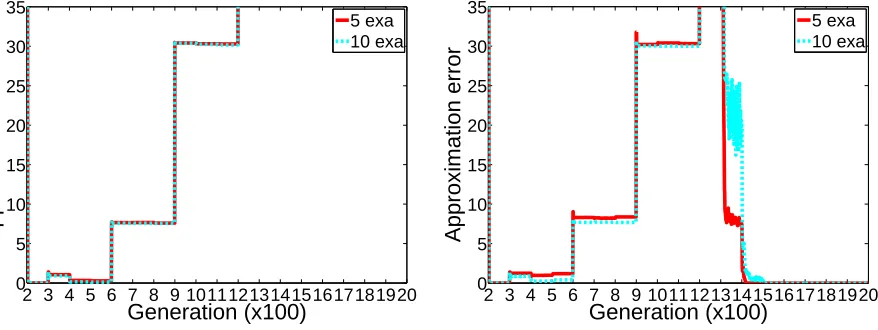
Fig. 2.2 and 2.3 report the results for the plain BC-EMO algorithm, for a baseline algorithm and for our BC-EMO extension, respectively, over the considered case study. The performance of the algorithms is measured in
2 3 4 5 6 7 8 9 1011121314151617181920 0 5 10 15 20 25 30 35 Generation (x100) Approximation error 5 exa 10 exa
2 3 4 5 6 7 8 9 1011121314151617181920 0 5 10 15 20 25 30 35 Generation (x100) Approximation error 5 exa 10 exa
Figure 2.2: Performance of the BC-EMO algorithm (left) and of the baseline algorithm (right).
2 3 4 5 6 7 8 9 1011121314151617181920 0 5 10 15 20 25 30 35 Generation (x100) Approximation error 5 exa 10 exa
Figure 2.3: Performance of the extension of BC-EMO to handle preference drift.
CHAPTER 2. HANDLING PREFERENCE DRIFT IN INTERACTIVE DECISION
MAKING 2.5. EXPERIMENTAL RESULTS
number of training examples per iteration (exa). Results are the medians over 500 runs with different random seeds for the search of the evolutionary algorithm.
At the generic i-th training iteration, the baseline algorithm retrains the learnt model using only the i-th batch of observable data. This is the only difference with the plain BC-EMO. Experimental results not reported here show the better performance obtained by discarding the previous training examples rather than discounting their cost by a fixed multiplicative factor in (0,1).
Fig. 2.2 (left) shows that the original version of BC-EMO cannot han-dle preference drift. The algorithm cannot track the changes of the user preferences: with the exception of the first drift, the performance of the algorithm keeps degrading each time the value function changes. After the last drift of the user preferences, the percent approximation error exceeds value 35%. This sub-optimal performance is caused by the lack of diversi-fication during the search phase of the algorithm: the genetic population “gets trapped” in the region surrounding the global minima of the first and the second value functions.
2.6. CONCLUSION
CHAPTER 2. HANDLING PREFERENCE DRIFT IN INTERACTIVE DECISION MAKING
As expected, the best results are observed for the extension of BC-EMO designed for handling preference drift. Even if three training iteration are not enough for the perfect recovery from the second concept drift, the favourite solution of the decision maker generated by her third preference drift is perfectly identified. In the case of 10 training examples per iteration, an approximation error smaller than 1% is obtained at generation 1100. An even faster recovery is observed from the fourth concept drift: two training iteration are required to approximate the new gold solution within an 1% approximation error. Note that, with the exception of the peak at generation 900 (corresponding to the third preference drift), the results tend to remain within 10% of the gold solution when 10 examples per iteration are provided.
2.6
Conclusion
This work addresses the problem of handling evolving preferences in in-teractive decision making. We modify BC-EMO, a recent multi-objective genetic algorithm based on pairwise preferences, by adapting its learning stage to learn under a concept drift. Our solution relies on the popular ap-proach of instance weighting, in which the relative importance of examples is adjusted according to their predicted relevance for the current concept. We integrate these modifications with a diversification strategy favouring exploration as a response to changing DM preferences. Experimental re-sults on a benchmark MOO problem with non-linear user preferences show the ability of the approach to early adapt to concept drifts.
CHAPTER 2. HANDLING PREFERENCE DRIFT IN INTERACTIVE DECISION
MAKING 2.6. CONCLUSION
2.6. CONCLUSION
Chapter 3
Active Learning of Combinatorial
Features for Interactive Optimization
3.1. INTRODUCTION
CHAPTER 3. ACTIVE LEARNING OF COMBINATORIAL FEATURES FOR INTERACTIVE OPTIMIZATION
3.1
Introduction
The field of combinatorial optimization focussed in the past mostly on solv-ing well defined problems, where the function f(x) to optimize is given, either in a closed form, or as a simulator which can be interrogated to de-liver f values corresponding to inputs, possibly with some noise leading to stochastic optimization. One therefore distinguishes two separated phases, a first one related to defining the problem through appropriate consulting, knowledge elicitation, modeling steps, and a second one dedicated to solv-ing the problem either optimally, in the few cases when this is possible, or approximately, in most real-world cases leading to NP-hard problems.
Unfortunately the above picture is not realistic in many application sce-narios, where learning about the problem definition goes hand in hand with delivering a set of solutions of improving quality, as judged by a decision maker (DM) responsible for selecting the final solution. In particular, this holds in the context of multi-objective optimization, where one aims at maximizing at the same time a set of functions f1, ..., fn. Multi-objective
optimization, when cast in the language of machine learning, is a paradig-matic case of lack of information, where only some relevant building blocks (features) are initially given as the individual function fi’s, but their
CHAPTER 3. ACTIVE LEARNING OF COMBINATORIAL FEATURES FOR
INTERACTIVE OPTIMIZATION 3.1. INTRODUCTION
than in delivering utility values. The interplay of optimization and ma-chine learning has been advocated in the past for example in the Reactive Search Optimization (RSO) context, see [2] also for an updated bibliog-raphy and [3] for an application of RSO in the context of multi-objective optimization.
In this work, we focus on a setting in which the optimal utility function
is bothunknown andcomplex enough to prevent exhaustive enumeration of
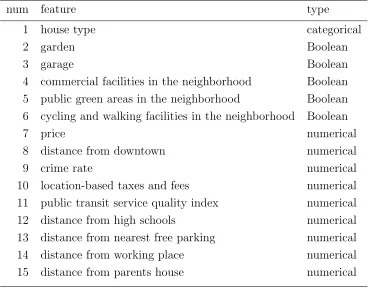
possible solutions. We start by considering combinatorial utility functions expressed as weighted combinations of terms, each term being a conjunc-tion of Boolean features. A typical scenario would be a house sale system suggesting candidate houses according to their characteristics, such as “the kitchen is roomy”, “the house has a garden”,“the neighbourhood is quiet”. The task can be formalized as a weighted MAX-SAT problem, a well-known formalization which allows to model a large number of real-world optimization problems. However, in the setting we consider here the un-derlying utility function is unknown and has to be jointly and interactively learned during the optimization process.
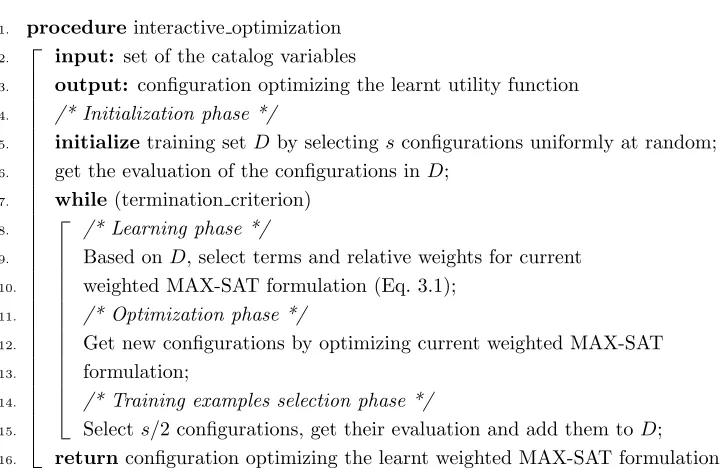
Our method consists of an iterative procedure alternating a search phase and a model refinement phase. At each step, the current approximation of the utility function is used to guide the search for optimal configurations; preference information is required for a subset of the recovered candidates, and the utility model is refined according to the feedback received. A set of randomly generated examples is employed to initialize the utility model at the first iteration.
3.2. OVERVIEW OF OUR APPROACH
CHAPTER 3. ACTIVE LEARNING OF COMBINATORIAL FEATURES FOR INTERACTIVE OPTIMIZATION
constraints. The generalization basically consists of replacing satisfiability with satisfiability modulo theory [1] (SMT). SMT is a powerful formalism combining first-order logic formulas and theories providing interpretations for the symbols involved, like the theory of arithmetic for dealing with integer or real numbers. It has received consistently increasing attention in recent years, thanks to a number of successful applications in areas like verification systems, planning and model checking.
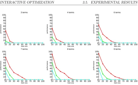
Experimental results on both weighted MAX-SAT and MAX-SMT prob-lems demonstrate the effectiveness of our approach in focusing towards the optimal solutions, its robustness as well as its ability to recover from sub-optimal initial choices.
The chapter is organized as follows: Section 3.2 introduces the algorithm for the SAT case. Section 3.3 introduces SMT and its weighted generaliza-tion and shows how to adapt our algorithm to this setting. Related works are discussed in Section 3.4. Section 3.5 reports the experimental evalu-ation for both SAT and SMT problems. A discussion including potential research directions concludes the chapter.
3.2
Overview of our approach
Candidate configurations are n dimensional Boolean vectors x consisting
of catalog features. The only assumption we make on the utility function is its sparsity, both in the number of features (from the whole set of catalog ones) and in the number of terms constructed from them. We rely on this assumption in designing our optimization algorithm.
CHAPTER 3. ACTIVE LEARNING OF COMBINATORIAL FEATURES FOR INTERACTIVE OPTIMIZATION 3.2. OVERVIEW OF OUR APPROACH
wp and 1−wp, respectively. A greedy move consists of flipping one of the variables leading to the maximum increase in the sum of the weights of the satisfied terms (if improving moves are not available, the least worsening move is accepted). The main difference w.r.t the “standard” weighted SLS algorithms consists of the DNF rather than CNF representation, which we believe to be a more natural choice when modeling combined effects of multiple non-linearly related features. Since switching from disjunctive to conjunctive normal form representations may involve an exponential in-crease in the size of the Boolean formula, we implemented a method that operates on formulae represented as a weighted linear sum of terms.
The candidate solutions generated by the optimizer during the search phase are first sorted by their predicted score values and then shuffled
uni-formly at random. The first s/2 configurations are selected, where s is
the number of the random training examples generated at the initializa-tion phase. The evaluainitializa-tion of the selected configurainitializa-tions completes the generation of the new training examples.
The refinement of the utility model consists of learning the weights of the terms, discarding the terms with zero weight. In the following, we assume that the available feedback consists of a quantitative score. We thus learn the utility function by performing regression over the set of the Boolean vectors. Adapting the method to other forms of feedback, such as ranking of sets of solutions, is straightforward as will be discussed in Section 3.6. We address the regression task by the Lasso [46]. The Lasso is an appropriate choice on problem domains with many irrelevant features, as its 1-norm regularization can automatically select input features by assigning zero weights to the irrelevant ones. Feature selection is crucial for achieving accurate prediction if the underlying model is sparse [19].
Let D = (xi, yi)i=1...m the set of m training examples, where xi is the
accom-3.2. OVERVIEW OF OUR APPROACH
CHAPTER 3. ACTIVE LEARNING OF COMBINATORIAL FEATURES FOR INTERACTIVE OPTIMIZATION
plished by solving the following lasso problem:
minw
m
X
i=1
(yi −wT ·Φ(xi))2 +λ||w||1 (3.1) where the mapping function Φ projects sample vectors to the space of all
possible conjunctions of up to d Boolean variables. The learnt function
f(x) = wT · Φ(x) will be used as the novel approximation of the util-ity function. A new iteration of our algorithm can now take place. The pseudocode of our algorithm is in Fig. 3.1.
In principle, one may argue that showing random examples to the user during the initialization phase (lines 5-6 in Fig. 3.1) is not an appropriate choice and may result a little bit artificial. However, the evaluation of diverse examples stimulates the preference expression, especially when the user is still uncertain about her final preference [37]. In particular, the diversity of the examples helps the user to reveal the hidden preferences: in many cases the decision maker is not aware of all preferences until she sees them violated. For example, a user does not usually think of stating the preference for an intermediate airport until one solution proposes an airplane change in a place she dislikes [37].
Note that dealing with the explicit projection Φ in Eq. 3.1 is tractable only for a rather limited number of catalog features and size of
conjunc-tions d. This will typically be the case when interacting with a human
DM. A possible alternative consists of directly learning a non-linear func-tion of the features, without explicitly projecting them to the resulting higher dimensional space. We do this by kernel ridge regression [42] (Krr), where 2-norm regularization is used in place of 1-norm. The resulting dual formulation can be kernelized into:
CHAPTER 3. ACTIVE LEARNING OF COMBINATORIAL FEATURES FOR INTERACTIVE OPTIMIZATION 3.2. OVERVIEW OF OUR APPROACH
1. procedureinteractive optimization 2. input: set of the catalog variables
3. output: configuration optimizing the learnt utility function 4. /* Initialization phase */
5. initializetraining setD by selectingsconfigurations uniformly at random;
6. get the evaluation of the configurations inD;
7. while(termination criterion) 8. /* Learning phase */
9. Based onD, select terms and relative weights for current
10. weighted MAX-SAT formulation (Eq. 3.1);
11. /* Optimization phase */
12. Get new configurations by optimizing current weighted MAX-SAT
13. formulation;
14. /* Training examples selection phase */
15. Selects/2 configurations, get their evaluation and add them toD;
16. returnconfiguration optimizing the learnt weighted MAX-SAT formulation
Figure 3.1: Pseudocode for the interactive optimization algorithm.
where K and I are the kernel and identity matrices respectively and λ is
again the regularization parameter. The learnt function is a linear combi-nation of kernel values between the example and each of the training in-stances: f(x) = Pm
i=1αiK(x,xi). We employ a Boolean kernel [26] which implicitly considers all conjunctions of up to d features:
KB(x,x′) =
d
X
l=1
xT ·x′
l
With the lasso, the function Φ(·) maps the Boolean variables to all
possible terms of size up to d. This allows for an explicit representation of the learnt utility function f as a weighted combination of the selected Boolean terms. On the other hand, in the kernel ridge regression case terms are only implicitly represented via the Boolean kernel KB. In both
cases, the value of the learnt function f is used to guide the search of
the SLS algorithm. In the following, the two proposed approaches are
3.3. SATISFIABILITY MODULO THEORY
CHAPTER 3. ACTIVE LEARNING OF COMBINATORIAL FEATURES FOR INTERACTIVE OPTIMIZATION
experimental section, the sparsity-inducing property of the Lasso allows it
to consistently outperform Krr. The problem of addressing more complex
scenarios, possibly involving non-human DM, where we can not afford an explicit projection, will be discussed in Section 3.6.
3.3
Satisfiability Modulo Theory
In the previous section, we assumed our optimization task could be cast into a propositional satisfiability problem. However, many applications of interest require or are more naturally described in more expressive log-ics as first-order logic (FOL), involving quantifiers, functions and predi-cates. In these cases, one is usually interested in validity of a FOL formula with respect to a certain background theory T fixing the interpretation of (some of the) predicate and function symbols. A general purpose FOL reasoning system such as Prolog, based on the resolution calculus, needs to add to the formula a conjunction of all the axioms in T. This is, for instance, the standard setting we consider in inductive logic programming when verifying whether a certain hypothesis covers an example given the available background knowledge. Whenever the cost of including such addi-tional background theory is affordable, our algorithm can be applied rather straighforwardly.
Unfortunately, adding all axioms of T is not viable for many theories of interest: consider for instance the theory of arithmetic, which restricts the interpretation of symbols such as +,≥,0,5. A more efficient alternative consists of using specialized reasoning methods for the background theory of interest. The resulting problem is known as satisfiability modulo theory
CHAPTER 3. ACTIVE LEARNING OF COMBINATORIAL FEATURES FOR INTERACTIVE OPTIMIZATION 3.3. SATISFIABILITY MODULO THEORY
in real-time embedded systems design. Popular examples of useful theories include various theories of arithmetic over reals or integers such as linear
or difference ones. Linear arithmetic considers + and − functions alone,
applied to either numerical constants or variables, plus multiplication by a numerical constant. Difference arithmetic is a fragment of linear arithmetic limiting legal predicates to the form x −y ≤ c, where x, y are variables and c is a numerical constant. Very efficient procedures exists for checking satisfiability of difference logic formulas [34].
A number of theories have been studied apart from standard arithmetic ones. Machine arithmetic, for instance, is more naturally modeled by the theory of bit-vector arithmetic, which includes bit-wise operations. The
theory of arrays includes two functionsread(a,i)andwrite(a,i,v). The
former returns the value of array a at index i, the latter an array identical
toa but for positionihaving value changed tov. This theory is extensively
used to model arrays in programs as well as an abstraction of memory. Other theories exists for data structures such as lists and strings.
3.3.1 Satisfiability Modulo Theory solvers
3.3. SATISFIABILITY MODULO THEORY
CHAPTER 3. ACTIVE LEARNING OF COMBINATORIAL FEATURES FOR INTERACTIVE OPTIMIZATION
1. procedureSMT-solver(ϕ) 2. ϕ′=α(ϕ)
3. while(true)
4. (r,M) ←SAT(ϕ′)
5. if r =unsat then returnunsat
6. (r,J) ←T-Solver(β(M))
7. if r =satthen returnsat
8. C←W
l∈J¬α(l)
9. ϕ′←ϕ′∧C
Figure 3.2: Pseudocode for a basic lazy SMT-solver.
until a solution satisfying both solvers is retrieved or the problem is found
to be unsatisfiable. Let ϕ be a formula in a certain theory T, made of a
set of n predicates A = {a1, . . . , an}. A mapping α maps ϕ into a
proposi-tional formula α(ϕ) by replacing its predicates with propositional variables pi = α(ai). The inverse mapping β replaces propositional variables with
their corresponding predicates, i.e., β(pi) = ai. For example, consider the
following formula in a non-linear theory T:
(cos(x) = 3 + sin(y))∧(z ≤ 8) (3.2)
Then, p1 = α(cos(x) = 3 + sin(y)) and p2 = α(ai ≤ 8). Note that the
truth assignment p1 = true, p2 = f alse is equivalent to the statement
(cos(x) = 3 + sin(y))∧ (z > 8) in the theory T.
Figure 3.2 reports the basic form [32] of an SMT algorithm. SAT(ϕ)
calls the SAT solver on the ϕ instance, returning a pair (r, M), where r is
sat if the instance is satisfiable, unsat otherwise. In the former case, M
is a truth assignment satisfying ϕ. T-Solver(S) calls the theory solver on
the formula S and returns a pair (r, J), where r indicates if the formula is satisfiable. If r =unsat, J is a justification for S, i.e any unsatisfiable
subset J ⊂ S. The next iteration calls the SAT solver on an extended
instance accounting for this justification.
CHAPTER 3. ACTIVE LEARNING OF COMBINATORIAL FEATURES FOR INTERACTIVE OPTIMIZATION 3.3. SATISFIABILITY MODULO THEORY
strategy, by pursuing a tighter integration between the two solvers. A common underlying idea is to prune the search space for the SAT solver by calling the theory solver on partial assignments and propagating its results. Finally, combination methods exist to jointly employ different theories, see [33] for a basic procedure.
3.3.2 Weighted MAX-SMT
Weighted SMT generalizes SMT problems much like weighted MAX-SAT does with MAX-SAT ones. While a body of works exist addressing weighted MAX-SAT problems, the former generalization has been tackled only re-cently and very few solvers have been developed [18, 35, 13]. The simplest formulation consists of adding a cost to each or part of the formulas to be jointly satisfied, and returning the assignment of variables minimizing the sum of the costs of the unsatisfied clauses, or a satisfying assignment if it exists. The following is a “weighted version” of Eq. 3.2:
5·(cos(x) = 3 + sin(y)) + 12·(z > 8) (3.3)
where 5 and 12 are the cost of the violation of the first and the second predicate, respectively.
Generalizing, consider a true utility function f expressed as a weighted sum of terms, where a term is the conjunction of up tod predicates defined over the variables in the theory T. The set of all n possible predicates
represents the search space S of the MAX-SAT solver integrated in the
MAX-SMT solver. Our approach learns an approximation ˆf of f and gets
one of its optimizers v from the MAX-SMT solver. The optimizer (and in
general each candidate solution in the theory T) identifies an assignment
p∗ = (p∗
1, . . . , p∗n) of Boolean values (p∗i = {true,false}) to the predicates
in S. The DM is asked for a feedback on the candidate solution v and
3.4. RELATED WORKS
CHAPTER 3. ACTIVE LEARNING OF COMBINATORIAL FEATURES FOR INTERACTIVE OPTIMIZATION
represents a new training example for our approach. In order to obtain multiple training examples, we optimize again ˆf with the additional hard1
constraint generated by the disjunction of all the terms of ˆf unsatisfied by
p∗ . For example, let t1 and t5 be the terms of ˆf unsatisfied by p∗, then the hard constraint becomes:
(t1 ∨ t5)
If p∗ satisfies all the terms of ˆf, i.e., ˆf(p∗) = 0, the additional hard con-straint generated is
(¬p∗1 ∨ ¬p∗2. . .∨ ¬p∗n)
which excludes p∗ from the feasible solutions set of ˆf. The generation of the training examples is iterated till the desired number of examples have been created or the hard constraints generated made the MAX-SMT problem unsatisfiable.
The learning component of our algorithm is then re-trained, including in the training set the new collected examples and the approximation of the true utility function is refined. A new optimization phase can now take place (see Fig. 3.1).
The mechanism creating the training examples is motivated by the tradeoff between the selection of good solutions (w.r.t. the current approx-imation of the true utility function) and the diversification of the search process.
3.4
Related works
Active learning is a hot research area and a broad range of different ap-proaches has been proposed (see [40] for a review). The simplest and most
1Hard constraints do not have a cost, and they have to be satisfied. On the contrary, the terms with
CHAPTER 3. ACTIVE LEARNING OF COMBINATORIAL FEATURES FOR
INTERACTIVE OPTIMIZATION 3.4. RELATED WORKS
common framework is that of uncertainty sampling: the learner queries
the instances on which it is least certain. However, the ultimate goal of a recommendation or optimization system is selecting the best instance(s) rather than correctly modeling the underlying utility function. The query strategy should thus tend to suggest good candidate solutions and still learn as much as possible from the feedback received. Typical areas where research on this issue is quite popular are single- and multi-objective inter-active optimization [7] and information retrieval [38]. The need to trade off multiple requirements in this active learning setting is addressed in [49] where the authors consider relevance, diversity and density in selecting
candidates. Note that our approach relies on query synthesis rather than
selection, as de-novo candidate solutions are generated by the SLS
algo-rithm. Nonetheless, our diversification strategies are very simple and could be significantly improved by taking advantage of the aforementioned liter-ature.
Choosing relevant features according to their weight within the learnt model is a common selection strategy (see e.g. [22]). When dealing with implicit feature spaces as in kernel machines, the problem can be ad-dressed by introducing a hyper-parameter for each input feature, like a
feature-dependent variance for Gaussian kernels [12]. Parameters and
hyper-parameters (or their relaxed real-valued version) are jointly opti-mized trying to identify a small number of relevant features. One-norm regularization [46] has the advantage of naturally inducing sparsity in the set of selected features. Approaches also exist [47, 24] which directly ad-dress the combinatorial problem of zero-norm optimization.
3.4. RELATED WORKS
CHAPTER 3. ACTIVE LEARNING OF COMBINATORIAL FEATURES FOR INTERACTIVE OPTIMIZATION
allows to deal with complex non-linear interactions between (Boolean) ob-jectives and, thanks to the SMT extension, can be applied to a wide range of optimization problems.
3.4.1 Constraint programming approaches for preference elici-tation
Very recent works in the field of constraint programming [21] define the user preferences in terms of soft constraints and introduce constraint op-timization problems where the data are not completely known before the solving process starts.
In soft constraints, a generalization of hard constraints, each assign-ment to the variables of one constraint is associated to a preference value taken from a preference set. The preference value represents the level of desirability of the assignment. The desirability of a complete assignment is computed by applying a combination operator to the local preference val-ues. A set of soft constraints generates an order (partial or total) over the complete assignments of the variables of the problem. Given two solutions of the problem, the preferred one is selected by computing their preference levels and by comparing them in the preference order. Soft constraints are therefore represented by an algebraic structure, called c-semiring (where letter “c” stays for “constraint”), providing two operations for combining (×) and comparing (+) preference values. In detail, the c-semiring is a tuple (A,+,×,0,1) where:
• A is a set and 0,1 ∈ A;
• + is commutative, associative and idempotent; 0 is its unit element
and 1 is its absorbing element;
CHAPTER 3. ACTIVE LEARNING OF COMBINATORIAL FEATURES FOR
INTERACTIVE OPTIMIZATION 3.4. RELATED WORKS
Note that a c-semiring is a semiring with additional properties for the two
operations: the operation + must be idempotent and with 0 as absorbing
element, the operation × must be commutative. The relation ≤A over
A, a ≤A b iff a +b = b, is a partial order, with 0 and 1 its minimum and
maximum elements, respectively. The relation≤A allows to compare (some
of) the desirability levels, with a ≤A b meaning thatb is “better” than a; 0
and 1 represent the worst and the best preference levels, respectively, and
the operations + and × are monotone on ≤A.
The c-semiring formalism can model just negative preferences. First,
the best element in the ordering induced by ≤A, denoted by 1, behaves
as indifference, since ∀a ∈ A,1 × a = a. This re