A scan statistic for continuous data based on the normal probability model

Open Access

Methodology

A scan statistic for continuous data based on the normal probability

model

Martin Kulldorff*

_{, Lan Huang}

_{and Kevin Konty}

Address: 1_{Department of Population Medicine, Harvard Medical School and Harvard Pilgrim Health Care Institute, Boston, MA 02215, USA,} 2_{National Cancer Institute, Bethesda, MD, USA; Currently at the United States Food and Drug Administration, Rockville, MD, USA and} 3_{New York}

City Department of Health and Mental Hygiene, New York City, NY, USA

Email: Martin Kulldorff* - [email protected]; Lan Huang - [email protected]; Kevin Konty - [email protected] * Corresponding author

Abstract

Temporal, spatial and space-time scan statistics are commonly used to detect and evaluate the statistical significance of temporal and/or geographical disease clusters, without any prior assumptions on the location, time period or size of those clusters. Scan statistics are mostly used for count data, such as disease incidence or mortality. Sometimes there is an interest in looking for clusters with respect to a continuous variable, such as lead levels in children or low birth weight. For such continuous data, we present a scan statistic where the likelihood is calculated using the the normal probability model. It may also be used for other distributions, while still maintaining the correct alpha level. In an application of the new method, we look for geographical clusters of low birth weight in New York City.

Background

Spatial and space-time scan statistics [1-4] have become popular methods in disease surveillance for the detection of disease clusters, and they are also used in many other fields. In most applications to date, the interest has been in count data such as disease incidence, mortality or prev-alence, for which a Poisson or Bernoulli distribution is used to model the random nature of the counts. For exam-ple, in papers published in 2008, Chen et al. [5] studied cervical cancer mortality in the United States; Osei and Duker [6] studied cholera prevalence in Ghana; Oeltmann et al. [7] looked at multidrug-resistant tuberculosis preva-lence in Thailand; Mohebbi at al. [8] studied gastrointes-tinal cancer incidence in Iran; Rubinsky-Elefant et al. [9] looked at human toxocariasis prevalence in Brazil; Frossling et al. [10] evaluated the Neospora caninum dis-tribution in dairy cattle in Sweden; Heres et al. [11] stud-ied mad-cow disease in the Netherlands; and Reinhardt et

al. [12] developed a system for prospective meningococcal disease incidence surveillance in Germany.

It is also of interest to detect spatial clusters of individuals or locations with high or low values of some continuous data attribute. Gay et al. [13] developed a spatial hazard model which they applied to detect geographical clusters of dietary cows with a high somatic cell score, which is a continuous marker for udder inflamation. Stoica et al. [14] has proposed a cluster detection method based on a number of random disks that jointly cover the cluster pat-tern in a marked point process. Huang [15] and Cook et al. [16] have developed spatial scan statistics for survival type data with censoring. The former applied the method to prostate cancer survival while the latter used their method for the time from birth until to asthma, allergic rhinitis or exczema. Other continuous data, such as birth weight [17] or blood lead levels, may be better modeled Published: 20 October 2009

International Journal of Health Geographics 2009, 8:58 doi:10.1186/1476-072X-8-58

Received: 30 July 2009 Accepted: 20 October 2009

This article is available from: http://www.ij-healthgeographics.com/content/8/1/58

© 2009 Kulldorff et al; licensee BioMed Central Ltd.

using a normal distribution, sometimes after a suitable transformation.

In this paper we develop a scan statistic for continuous data that is based on the normal probability model. Under the null hypothesis, all observations come from the same distribution. Under the alternative hypothesis, there is one cluster location where the observations have either a larger or smaller mean than outside that cluster. A key feature of the method is that the statistical inference is still valid even if the true distribution is not normal, assur-ing that the correct alpha level is maintained. This is accomplished by evaluating the statistical significance of clusters through a permutation based Monte Carlo hypothesis testing procedure. The new method is applied to birth weight data from New York City. A simulation study is performed to evaluate the power for different types of clusters.

The application and simulation results presented in this paper are concerned with two-dimensional spatial data, using a circular variable size scanning window. The new method is equally applicable to purely temporal and spa-tio-temporal data [18-20], to be used for daily prospective disease surveillance to look for suddenly emerging clus-ters. In addition to circles, it may also be used with an elliptic scanning window [21], or with any collection of non-parametric shapes [2,22-25].

The normal model has been incorporated into the freely available SaTScan software http://www.satscan.org for spatial and sdpace-time scan statistics, so it is easy to use. While it requires the use of computer intensive Monte Carlo simulations, computing times are very reasonable, unless the data set is huge.

A Spatial Scan Statistic for Normal Data

The data consists of a number of continuous observations, such as birth weight, with values x_i, i = 1,...,N. Each obser-vation is at a spatial location s, s = 1,...,S, with spatial lati-tude and longilati-tude coordinates lat(s) and long(s). Each location has one or more observations, so that S ≤N. For each location s, define the sum of the observed values as x_s = ∑_i∈s xi and the number of observations in the

loca-tion as ns The sum of all the observed values are X = ∑ixi.

Scanning Window

The circular spatial scan statistic is defined through a large number of overlapping circles [18]. For each circle z, a log likelihood ratio LLR(z) is calculated, and the test statistic is defined as the maximum LLR over all circles. The scan-ning window will depend on the application, but it is typ-ical to define the window as all circles centered on an

observation and with a radius varying continuously from zero up to some upper limit. To ensure that both small and large clusters can be found, the upper limit is often defined so that the circle contains at most 50 percent of all observations. It is never set above that number though, since a circular cluster with high values covering for exam-ple 80 percent of all observations is more appropriatly interpreted as a spatially disconnected 'cluster' with low values covering the 20 percent of observations that are located outside the circle, since it is those 20 percent that differ from the majority of observations. The maximum cluster size can also be defined using specific units of dis-tance (e.g., 10 km). Circles with only one observation are ignored. Let n_z = ∑_s∈zns be the number of observations in

circle z, and let xz = ∑s∈zxs be the sum of the observed

val-ues in circle z.

Likelihood Calculations

Under the null hypothesis, the maximum likelihood esti-mates of the mean and variance are μ = X/N and

respectively. The likelihood under the

null hypothesis is then

and the log likelihood is

Under the alternative hypothesis, we first calculate the maximum likelihood estimators that are specific to each circle z, which is μz = xz/nz for the mean inside the circle

and λ_z = (X - x_z)/(N - n_z) for the mean outside the circle. The maximum likelihood estimate for the common vari-ance is

The log likelihood for circle z is σ2₌ ∑i(μ−xi)2

N L e xi i 0 1 2 2 2 2 = − −

∏

μ σ

( )

lnL Nln Nln xi

i

0 2

2

2 2

= − ( π)− ( )σ −

∑

σ μ μ

λ λ

z i z z z z

i z

i z z z z

i z

N x x n

x X x N n

2 2 2

This simplifies to

As the test statistic we use the maximum likelihood ratio

or more conveniently, but equivalently, the maximum log likelihood ratio

Only the last term depends on z, so from this formula it can be seen that the most likely cluster selected is the one that minimizes the variance under the alternative hypoth-esis, which is intuitive.

Randomization

The statistical significance of the most likely cluster is eval-uated using Monte Carlo hypothesis testing [26]. Rather than generating random data from the normal distribu-tion, a large set of random data sets are created by ran-domly permuting the observed values x_i and their corresponding locations s. That is, the analysis is condi-tioned on the collection of continuous observations that were observed, as well as on the locations at which they were observed, which are considered non-random. By doing the randomization this way, the correct alpha level will be maintained even if the observations do not truly come from a normal distribution. Note that it is the indi-vidual observations that are permuted, so two different observations in the same location will end up in two dif-ferent locations in most of the random data sets.

For each random data set, the log likelihood lnL(z) is cal-culated for each circle. The most likely cluster is then found and its log likelihood ratio is noted. If the log like-lihood ratio from the real data set is among the 5 percent highest of all the data set, then the most likely cluster from the real data set is statistically significant at the 0.05 alpha level. More specifically, if there are M random data sets, then the p-value of the most likely cluster is R/(M + 1), where R is the rank of the log likelihood ratio from the real data set in comparison with all data sets. In order to obtain nice p-values with a finite number of decimals, M

should be chosen as for example 999, 4999 or 99999.

Note that these Monte Carlo based p-values are exact in the sense that under the null hypothesis, the probability of observing a p-value less than or equal to p is exactly p

[26]. This is true irrespective of the number of random data sets M, but a higher M will provide higher statistical power.

If the random simulated data had instead been generated from a normal distribution with pre-specified mean and variance, rather than through permutation, then one would test the null hypothesis that the observations come from exactly that normal distribution. We would then reject the null for many reasons other than the existance of spatial clusters. For example, the null may be rejected because the mean values are higher than specified uni-formly throughout the whole study region.

Scanning for High or Low Values

As defined above, the normal scan statistic will search for clusters with exceptionally high values as well as clusters with exceptionally low values. Sometimes it makes more sense to only search for clusters with high values. The former is easily accomplished by adding an indicator function I(μ_z >λ_z) to the likelihood that is calculated under the alternative hypothesis. If one is only interested in cluster with low values, the indicator function is instead

I(μ_z <λ_z).

Software

The normal scan statistic has been incorporated into the freely available SaTScan™ software package, version 7.0 http://www.satscan.org. It can be used for temporal, spa-tial and/or spatio-temporal data. The spaspa-tial version may be applied using a circular or elliptic window in two dimensions or a spheric window in three or more dimen-sions. The space-time version uses a cylindrical scanning window with either a circular or elliptic base. It is also pos-sible for the user to define his/her own non-Euclidian neighborhood metric. The circle centroids can be identical to the collection of coordinates of the observations, or they may be specified by the user.

lnL z Nln Nln

z

x x n

x

z

i z z z z i z i ( )= − ( )− ( ) − ⎛ − + ⎝ ⎜ ⎜ + − ∈

∑

σ μ μ

2

2(X x_z) _z (N n_z) _z2

i z − + − ⎞ ⎠ ⎟ ⎟ ∉

∑

lnL z( )= −Nln( 2π)−Nln( σ_z2)−N/2

max /

z Lz L0

max( / )

max ( ) ( ) /

( ) ( )

z z

z z

lnL lnL

Nln Nln N

Nln Nln 0 2 2 2 2 =

(

π σ (( )

max ( ) ( ) ( )

xi

Nln xi N Nln

i z z i − ⎞ ⎠ ⎟ ⎟ = ⎛ + − − − ⎝ ⎜ ⎜ ⎞

∑

∑

2 2 2

2

Detection of Low Birth Weight and Early

Gestation Clusters in New York City

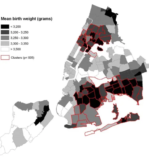
The New York City Department of Health and Mental Hygiene (NYCDOH) calculates infant mortality rates by neighborhood and reports them in its annual Summary of Vital Statistics [27]. Though the infant mortality rate has fallen dramatically over the past 20 years (from 13.4 per 1000 in 1988 to 5.4 per 1000 in 2007) neighborhood var-iation can be quite high and this has attracted much atten-tion from public health officials, the press, and researchers [28-30]. One approach to understanding the spatial pattern of infant mortality is to investigate the spa-tial patterns of known risk factors such as low birth weight, early gestation, or congenital conditions [28-30,17,31,32]. Attempts to identify clusters of low birth weight typically rely on dichotomized variables for birth weight (low: < 2500 grams; very-low: < 1500 grams) [17,31]. However, some researchers have noted a more complicated relationship among birth weight, gestation, and infant mortality with risk varying considerably within low birth weight and early gestation categories and modi-fied by gender and other demographic characteristics [32].

This section examines spatial patterns of continuous measures of birth weight in New York City, using the spa-tial scan statistic with the normal probability model. Vital Records from NYCDOH were used to obtain data for all singleton births occurring in New York City in 2004. Births were geo-referenced to the Mother's zip code. Births to mother's not residing in New York City and those with invalid zips were deleted. Birth weight was measured in grams. The normal spatial scan statistic was used to detect clusters of low birth weight, using a circular window shape and 50 percent of all birth as the maximum cluster size.

Two statistically significant geographical clusters of low birth weight were found (Table 1 and Figure 1). With a log likelihood ratio (LLR) of 125.8, the first one consists of 61 zip-code areas in eastern Brooklyn and southern Queens, where the birth weights were on average 60 grams less than the rest of the city (p < 0.001). The second cluster consists of 29 zip-code areas in northern Manhattan and southern Bronx, where the birth weights were on average 52 grams less (LLR = 62.7, p < 0.001). The two statistically significant clusters correspond closely to areas of increased risk for infant mortality and are highly corre-lated with clusters found using dichotomized variables. There was also a non-significant single zip-code cluster on Staten Island (60 grams less, LLR = 3.6, p = 0.90). Note that, while the weight difference is as large or larger in the State Island cluster, such a difference could easily be due to chance, due to the small number of births inside the cluster. Note also that since a circular scanning window is used, some low birth weight areas are just outside the

Brooklyn-Queens cluster while some high birth weigth areas are just inside. The key thing to realize is that it is only the general area of the cluster that is detected, not its exact boundaries.

For the City as a whole, the variance of the birth weights is 297250 and the standard deviation is 545.2. After accounting for the different means inside and outside of the most likely cluster, the variance is 296564 and the standard deviation is 544.6. These number are, by default, lower, but only marginally so. In fact, the most likely clus-ter only explains (297250 - 296564)/297250 = 0.23 per-cent of the total variance. This is not surprising for an outcome such as birth weight, since the natural variation is rather large.

The spatial pattern of birth weight may be largely driven by the spatial patterns of demographic and pregnancy-specific characteristics. If so, clusters are not surprising; simply reflecting the geographical distribution of known characteristics. As such, the public health utility of cluster-ing in the raw data may be limited. In a substantive paper, we hope to reexamine the geographical clusters of birth weight adjusting for the mother's demographics, health status, and pregnancy characteristics that are known to correspond with low birth weight. This has two uses: first, it sharpens understanding of the relationship between demographic covariates and birth weight and second, it identifies areas with surprisingly low birth weight for investigation, which cannot be explained in terms of their underlying demographics.

Statistical Power and Spatial Precision

To evaluate the statistical power of the new method, we performed a simple simulation study. We simulated ran-dom normally distributed weights for infants born in New York City. The power to detect a cluster will depend on a number of factors, so data were generated using one standard baseline scenario and several variations: using different cluster locations within New York City, different cluster sizes, different sample size (total numbers of births), with different mean weights inside and outside the cluster, and with different variances inside and outside the true cluster.

We selected four cluster locations to have lower than aver-age birth weight. These are shown in Figure 2. Cluster No. 1 is the baseline cluster, located in the center of Brooklyn. Cluster No. 2 is centered on The Rockaways, Queens, close to the Atlantic Ocean. Cluster No. 3 is located on Staten Island, far away from the rest of the City. Cluster No. 4 is

split between southern Bronx and northern Queens. As the baseline, the maximum size of the clusters was defined to include 10 percent of all the births in the City. This means that the geographical size of the clusters varied, depending on the population density around the cluster centroid. For Cluster No. 1, we also evaluated clusters with The geographical distribution of birth weight in New York City zip codes in 2004, with two statistically significant clusters found by the spatial scan statistic with the normal probability model

Figure 1

Table 1: Geographical clusters of low birth weight in New York City in 2004.

Inside Cluster Outside Cluster Weight

Cluster #Births Mean Weight (g) #Births Mean Weight (g) Difference (g) P-value

Brooklyn/Queens 27772 3236 81152 3296 60 0.001

Manhattan/Bronx 16258 3236 92666 3288 52 0.001

Staten Island 617 3221 108307 3281 60 0.90

The location and size of the artificial low birth weight clusters used to evaluate the statistical power of the spatial scan statistic for normally distributed data

Figure 2

The location and size of the artificial low birth weight clusters used to evaluate the statistical power of the spa-tial scan statistic for normally distributed data.

4

3

2

5 and 20 percent of the total number of births (dotted lines), while keeping the cluster centroid the same.

Let Z denote the collection of census tracts in the true clus-ter and let Zc _{denote the remaining New York City census}

tracts. For each of either 300, 600 (baseline), 900 or 1200 infants, we randomly simulate the birth weight from a normal distribution N(μ_Z, σ2_{) if the infant was born}

inside the cluster and from N( , σ2_{) if the infant was}

born outside the cluster. For all simulations, we set =

3250. We always choose μ_Z < , so that the simulated data has a cluster of low birth weight. For the baseline, we chose μ_Z to be ten percent less than , so that μ_Z = 3250

- 325 = 2925. We also evaluated clusters where μ_Z was 5, 8, 13, 15 and 20 percent less than . The variance σ2

was the same inside and outside the cluster. For the base-line model we set the standard deviation to σ= 600, but we also evaluated σ= 300 and σ= 900. A complete list of

all the evaluated cluster parameters are shown in the first five columns of Table 2.

For each cluster scenario, we simulated 1000 random data sets. The estimated power is calculated as the proportion of the 1000 random data sets for which the null hypothe-sis was rejected, expressed as a percentage.

Even when the null hypothesis is correctly rejected, the detected cluster is usually not exactly identical to the true cluster. The extant of the overlap, and hence, of the spatial accuracy of the detected cluster, can be evaluated using sensitivity and positive predicted value (PPV). The sensi-tivity is de-fined as the proportion of the infants in the true cluster that was included in the detected cluster. This obviously varies between the random data sets, and the estimated sensitivity is taken as the average over the 1000 random data sets. The positive predictive value is defined as the proportion of the infants in the detected cluster that are in the true cluster. Again, this is estimated by taking the average over the 1000 random data sets.

μ

Zc

μ_Zc μ

Zc

μ

Zc

μ_Zc

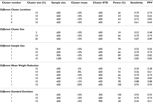
Table 2: Estimated power, sensitivity and positive predictive value (PPV) when the normal scan statistic is used to detect different types of clusters, as described in the text.

Cluster number Cluster size (%) Sample size Cluster mean Cluster STD Power (%) Sensitivity PPV

Different Cluster Locations

1 10 600 -10% 600 66 0.70 0.74

2 10 600 -10% 600 54 0.56 0.65

3 10 600 -10% 600 64 0.72 0.82

4 10 600 -10% 600 61 0.61 0.64

Different Cluster Size

1 5 600 -10% 600 34 0.52 0.48

1 10 600 -10% 600 66 0.70 0.74

1 20 600 -10% 600 96 0.87 0.89

Different Sample Size

1 10 300 -10% 600 34 0.55 0.56

1 10 600 -10% 600 66 0.70 0.74

1 10 900 -10% 600 89 0.83 0.82

1 10 1200 -10% 600 98 0.85 0.85

Different Mean Weight Reduction

1 10 600 -5% 600 14 0.30 0.38

1 10 600 -8% 600 42 0.56 0.61

1 10 600 -10% 600 66 0.70 0.74

1 10 600 -13% 600 92 0.84 0.84

1 10 600 -15% 600 98 0.88 0.88

1 10 600 -20% 600 100 0.93 0.93

Different Standard Deviation

1 10 600 -10% 300 100 0.93 0.93

1 10 600 -10% 600 66 0.70 0.74

The results are presented in Table 2. The power is approx-imately the same for the four different cluster locations, which is a reflection of the fact that they are about the same population size. As expected, the power increase when the cluster size increase, when the sample size increase, when the mean weight difference increase and when the standard deviation decrease. Sensitivity and pos-itive predictive value follow the same pattern. Note that the sensitivity is about the same as the positive predictive value. This means that we are about equally likely to leave out an infant that should be in the cluster as we are to include an infant that shouldn't be in the cluster. Note also that even when the power is 100, the sensitivity and positive predictive value are not. This means that while we can determine the general location of a cluster, there will almost always be uncertainty when it comes to the bor-ders of the detected cluster.

Discussion

We have presented a scan statistic for continuous data. It is based on the normal distribution function, so if the data is truly normal, we have a likelihood ratio test. If the data follows some other distribution, it is no longer a likeli-hood ratio test, but it still maintains the correct alpha level. Hence, it can be used for a wide variety of continu-ous data, although we do not recommend it for exponen-tial or other types of survival data, for which there are other scan statistics available [15,16].

The normal scan statistic performed well for the New York City birth weight data, finding two statistically significant clusters that corresponded to areas with high infant mor-tality.

The statistical power varies predictably with the type of cluster to be found. The same is true for sensitivity and the positive predictive value. One limitation of the simulation study is that we only evaluated the performance on data that were simulated from the normal distribution. While we know that the alpha level is correct for other distribu-tions, we do not know about the power, sensitivity and positive predictive value.

As with most other scan statistics, the method is computer intensive, but not prohibitively so. The freely available SaTScan™ software http://www.satscan.org is available to do the calculations in a purely temporal, purely spatial or space-time setting, and when looking for clusters with either only high or only low values, or simultaneously for both. The normal probability model has been available in the SaTScan software since 2006, and the method has already been applied to study the epidemics of classical swine fever in Spain [33], the geographical differences in respondent and non-respondents in epidemiological studies [34] and the geographical clustering of the time

people spend walking and bicycling in Los Angeles and San Diego [35]. The method can also be used in other fields outside of medicine and public health. For example, the variable of interest could be the amount of rainfall in various geographical locations in a country, pollution lev-els in a city, the height of plants on a field or the size of stars in a galaxy.

Competing interests

The authors declare that they have no competing interests.

Authors' contributions

MK obtained funding and developed the statistical meth-ods. KK selected and performed the SaTScan analysis on the real data. MK and LH designed and LH performed the simulated power evaluations. MK, KK and LH wrote the first draft for different parts of the manuscript. All authors revised the manuscript and approved the final version.

Acknowledgements

This work was funded by the National Institute of Child Health and Devel-opment, National Institutes of Health, grant number R01HD048852.

References

1. Naus J: Clustering of random points in two dimensions.

Biometrika 1965, 52:263-267.

2. Kulldorff M: A spatial scan statistic. Communications in Statistics: Theory and Methods 1997, 26:1481-1496.

3. Glaz J, Balakrishnan N, editors: Scan Statistics and Applications. Birkäus-er 1999.

4. Glaz J, Naus J, Wallenstein S: Scan Statistics Springer; 2001. 5. Chen J, Roth RE, Naito AT, Lengerich EJ, MacEachren AM:

Geovi-sual analytics to enhance spatial scan statistic interpretation: An analysis of US cervical cancer mortality. International Journal of Health Geographics 2008, 7:57.

6. Osei FB, Duker AA: Spatial dependency of V. cholera preva-lence on open space refuse dumps in Kumasi, Ghana: A spa-tial statistical modeling. International Journal of Health Geographics

2008, 7:62.

7. Oeltmann JE, Varma JK, Ortega L, Liu Y, O'Rourke T, Cano M, Har-rington T, Toney S, Jones W, Karuchit S, Diem L, Rienthong D, Tap-pero JW, Ijaz K, Maloney S: Multidrug-resistant tuberculosis outbreak among US-bound Hmong refugees, Thailand, 2005. Emerging Infectious Diseases 2008, 14:1715-1721.

8. Mohebbi M, Mahmoodi M, Wolfe R, Nourijelyani K, Mohammad K, Zeraati1 H, Fotouhi A: Geographical spread of gastrointestinal tract cancer incidence in the Caspian Sea region of Iran: Spa-tial analysis of cancer registry data. BMC Cancer 2008, 8:137. 9. Rubinsky-Elefant G, Silva-Nunes M, Malafronte RS, Muniz PT, Ferreira

MU: Human toxocariasis in rural Brazilian Amazonia: Sero-prevalence, risk factors, and spatial distribution. American Jour-nal of Tropical Medicine and Hygiene 2008, 79:93-98.

10. Frossling J, Nodtvedt A, Lindberg A, Björkman C: Spatial analysis of Neospora caninum distribution in dairy cattle from Swe-den. Geospa-tial Health 2008, 3:39-45.

11. Heres L, Brus DJ, Hagenaars TJ: Spatial analysis of BSE cases in the Netherlands. BMC Veterinary Research 2008, 4:21.

12. Reinhardt M, Elias J, Albert J, Frosch M, Harmsen D, Vogel U: EpiS-canGIS: An online geographic surveillance system for menin-gococcal disease. International Journal of Health Geographics 2008, 7:33.

13. Gay E, Senoussi R, Barnouin J: A spatial hazard model for cluster detection on continuous indicators of disease: Application to somatic cell score. Veterinary Research 2007, 38:585-596. 14. Stoica RS, Gay E, Kretzschmar A: Cluster pattern detection in

spatial data based on Monte Carlo inference. Biometrical Journal

Publish with BioMed Central and every scientist can read your work free of charge "BioMed Central will be the most significant development for disseminating the results of biomedical researc h in our lifetime."

Sir Paul Nurse, Cancer Research UK

Your research papers will be:

available free of charge to the entire biomedical community

peer reviewed and published immediately upon acceptance

cited in PubMed and archived on PubMed Central

yours — you keep the copyright

Submit your manuscript here:

http://www.biomedcentral.com/info/publishing_adv.asp

BioMedcentral 15. Huang L, Kulldorff M, Gregorio D: A spatial scan statistic for

sur-vival data. Biometrics 2007, 63:109-118.

16. Cook A, Gold DR, Li Y: Spatial cluster detection for censored outcome data. Biometrics 2007, 63:540-549.

17. Ozdenerol E, Williams BL, Kang SY, Magsumbol MS: Comparison of spatial scan statistic and spatial filtering in estimating low birth weight clusters. International Journal of Health Geographics

2005, 4:19.

18. Kulldorff M, Athas W, Feuer E, Miller B, Key C: Evaluating cluster alarms: A space-time scan statistics and brain cancer in Los Alamos. American Journal of Public Health 1998, 88:1377-1380. 19. Kulldorff M: Prospective time-periodic geographical disease

surveillance using a scan statistic. Journal of the Royal Statistical Society Series A 2001, 164:61-72.

20. Kulldorff M, Heffernan R, Hartman J, Assunção R, Mostashari F: A space-time permutation scan statistic for the early detection of disease outbreaks. PLoS Medicine 2005, 2:e59.

21. Kulldorff M, Huang L, Pickle L, Duczmal L: An elliptic spatial scan statistic. Statistics in Medicine 2006, 25:3929-3943.

22. Patil GP, Taillie C: Geographic and network surveillance via scan statistics for critical area detection. Statistical Science 2003, 18:457-465.

23. Duczmal L, Assunçao R: A simulated annealing strategy for the detection of arbitrarily shaped spatial clusters. Computational Statistics and Data Analysis 2004, 45:269-286.

24. Tango T, Takahashi K: A flexibly shaped spatial scan statistic for detecting clusters. International Journal of Health Geographics 2005, 4:11.

25. Assunçao RM, Costa M, Tavares A, Ferreira S: Fast detection of arbitrarily shaped disease clusters. Statistics in Medicine 2006, 25:723-742.

26. Dwass M: Modified randomization tests for nonparametric hypotheses. Annals of Mathematical Statistics 1957, 28:181-187. 27. Office of Vital Statistics: Summary of Vital Statistics 2004, the City of New

York. New York New York: New York City Department of Health; 2004.

28. Sohler NL, Arno PS, Chang CJ, Fang J, Schechter C: Income ine-quality and infant mortality in New York City. Urban Health

2003, 80:650-657.

29. Grady SC, McLafferty S: Disentangling the effects of residential segregation and neighborhood poverty on low birthweight for immigrant and native-born black women in New York City. Urban Geography 2007, 28:377-397.

30. Grady SC: Racial disparities in low birthweight and the contri-bution of residential segregation: A multilevel analysis. Social Science and Medicine 2006, 63:3013-3029.

31. Rushton G, Krishnamurthy R, Krishnamurt R, Lolonis P, Song H: The spatial relationship between infant mortality and birth defect rates in a U.S. city. Statistics in Medicine 1996, 15:1907-1919.

32. Solis P, Pullman SG, Frisbie WP: Demographic models of birth outcomes and infant mortality: An alternative measurement approach. Demography 2000, 37:489-498.

33. Martínez-López B, Perez AM, Sánchez-Vizcaíno JM: A stochastic model to quantify the risk of introduction of classical swine fever virus through import of domestic and wild boars. Epi-demiology and Infection 2009, 137:1505-1515.

34. Shen M, Cozen W, Huang L, Colt J, De Roos AJ, Severson RK, Cerhan JR, Bernstein L, Morton LM, Pickle L, Ward MH: Census and geo-graphic differences between respondents and nonrespond-ents in a case-control study of non-Hodgkin lymphoma.

American Journal of Preventive Medicine 2008, 167:350-361.

35. Huang L, Stinchcomb D, Pickle L, Dill J, Berrigan D: Identifying clus-ters of active transportation using spatial scan statistics.