Array Processing Techniques for Broadband Acoustic Beamforming

(1)

University of New Orleans University of New Orleans

ScholarWorks@UNO

University of New Orleans Theses and

Dissertations Dissertations and Theses

5-20-2005

Array Processing Techniques for Broadband Acoustic

Beamforming

Ryan Thiel

University of New Orleans

Follow this and additional works at: https://scholarworks.uno.edu/td

Recommended Citation Recommended Citation

Thiel, Ryan, "Array Processing Techniques for Broadband Acoustic Beamforming" (2005). University of New Orleans Theses and Dissertations. 251.

https://scholarworks.uno.edu/td/251

(2)

ARRAY PROCESSING TECHNIQUES FOR BROADBAND ACOUSTIC BEAMFORMING

A Thesis

Submitted to the Graduate Faculty of the University of New Orleans

in partial fulfillment of the requirements for the degree of

Master of Science in

The Department of Electrical Engineering

by

Ryan D. Thiel

(3)

ACKNOWLEDGEMENTS

I would like to thank Kenny Lannes, my thesis advisor, who provided the

ideas and motivation which started the thesis. His dedication made this work

possible. I would also like to thank Dr. Dimitrios Charalampidis and Dr. Vesselin

Jilkov for serving on my thesis committee.

Sincere appreciation goes to my parents Stephen and Vicki Thiel for

providing support and motivation throughout my education. I would also like to

thank Christopher Duggan, a fellow electrical engineer and good friend, who

carefully proofread this document many times throughout its development.

Finally, very special thanks goes to my fiancé Katherine Green for her love,

(4)

TABLE OF CONTENTS

LIST OF FIGURES ... iv

ABSTRACT... v

CHAPTER 1. Introduction... 1

2. Overview of Beamforming ... 3

2.1 Narrowband Beamforming ... 3

2.2 Broadband Beamforming... 6

3. Techniques ... 9

3.1 Frequency Up-Conversion... 9

3.1.1 Description... 9

3.1.2 Analysis ... 10

3.1.3 Results... 12

3.2 Decimation... 13

3.2.2 Analysis ... 14

3.3 Group Delay Discrimination... 17

3.3.2 Analysis ... 19

3.3.3 Implementation ... 22

3.3.4 Results... 24

4. Conclusions... 34

REFERENCES ... 36

APPENDIX... 37

(5)

LIST OF FIGURES

2.1 Typical Narrowband Array Beamformer ... 4

2.2 Two Element Narrowband Array and Beamformer ... 5

2.3 Two Element Narrowband Array Directivity Patterns... 5

2.4 Variation of Directivity Pattern Over a Large Bandwidth ... 6

2.5 Typical Broadband Beamformer ... 8

3.1 Frequency Up-Conversion Technique... 11

3.2 Single Side-Band Frequency Up-Conversion Technique... 12

3.3 Decimation in Time ... 14

3.4 Decimation With and Without a Reference Point ... 16

3.5 Group Delay Discrimination Process ... 19

3.6 Frequency Content of Group Delay Algorithm Test Signals ... 30

3.7 Test 4 Input and Output Comparison... 32

(6)

ABSTRACT

Audio acquisition and recording can benefit from directional reception of the

acoustic signals. Current acoustic designs of highly-directional microphones are

bandwidth limited and physically large. A microphone array used in conjunction

with a beamforming algorithm can acquire and spatially filter the signal, but

traditionally this has suffered from limitations similar to those of the purely

acoustic designs. The work presented in this paper attempts to overcome these

limitations by producing and analyzing three atypical techniques for broadband

beamforming. The last and most successful technique employs an algorithm

which calculates the difference in group delay of the acquired signals and uses that

information to determine the direction of the incoming signals as a function of

(7)

CHAPTER 1

INTRODUCTION

In film production, theater, news coverage, sports broadcasting, and nature

recording, audio must be recorded from a desired source without interference from

other audio sources. Placing a microphone close to the desired source is the

simplest way to reduce background interference but is often impractical. Common

solutions require directional microphones. Directional microphones have pickup

patterns which favor on-axis and reject off-axis acoustic energy. A wide

assortment of microphone pickup patterns is available ranging from

omni-directional to cardioid to super-cardioid to hyper-cardioid. In order to achieve the

more extreme pickup patterns, many expensive tradeoffs with other areas of

microphone performance, such as bandwidth, are made, so highly-directional

microphone performance leaves much to be desired.

A highly-directional microphone placed far from the source can pick up the

desired signal while reducing background interference, but highly-directional

microphones of the current generation have many shortcomings. The most

commonly used highly-directional microphones rely on either parabolic reflectors

or acoustical tubes (shotgun microphones) developed in the 1920s and 1930s to

focus on-axis or reject off-axis acoustic energy [1]. Attempts to move the sound

(8)

techniques. Using a microphone array has many advantages over an acoustic

approach but, with current array processing methods, array techniques suffer from

many of the same tradeoffs as the acoustic methods. Coloration of the sound, poor

low frequency rejection, inconsistent pickup pattern over bandwidth, and large

physical size are the drawbacks of these schemes. These drawbacks provide

motivation for the search for new techniques of acquiring audio data directionally.

Due to the wide availability of low-cost, high performance digital signal

processors and the versatile nature of beamforming, array processing seems the

best avenue to explore. Because the current beamforming methods available

suffer from some of the same drawbacks as the conventional methods for

highly-directional miking, new beamforming signal processing techniques are needed.

The new beamforming techniques should allow for a small array to process a large

bandwidth and provide a consistent narrow beamform over the bandwidth.

This thesis documents a search for these new techniques. An overview of

beamforming is presented in Chapter 2, and analyses of three attempts at new

beamforming techniques are presented in Chapter 3. These include Frequency

Up-Conversion (3.1), Non-Linear Decimation (3.2), and Group Delay

Discrimination (3.3). Chapter 4 concludes with a discussion of the effectiveness

(9)

CHAPTER 2

BEAMFORMING BACKGROUND

Beamforming is a method of processing data from an array of transducers

to achieve spatial filtering. The spatial filtering is used to acquire signals from a

particular direction while reducing interference from another. Beamforming can

be applied to either receiving or transmitting arrays and has applications in radar,

sonar, communications, imaging, geophysics, astrophysics, medicine, and more

[2]. The discussion here is limited to beamforming as it applies to receiving

arrays.

2.1 Narrowband Beamforming

Narrowband beamforming is used when the wanted signal occupies a

known narrow bandwidth. Any interference outside of that bandwidth can be

reduced with a temporal (as opposed to spatial) filter. If interference is expected

to occupy the same bandwidth but come from a different direction than the desired

signal, a beamformer can be useful. Signals from a spatial array of sensors can be

combined in such a way to enhance the signal coming from one direction and

reduce signal from another. The combination of the signals, for the narrowband

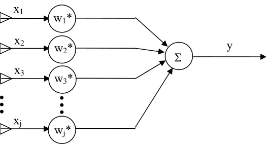
case, is usually a sum of weighted, phase shifted signals [3]. Differences in the

(10)

weights are usually complex numbers and represent both changes in phase and

magnitude. A typical narrowband array beamformer is shown in Figure 2.1.

Figure 2.1. Typical Narrowband Array Beamformer

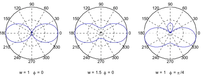
The simple two element array shown in Figure 2.2 has sensor spacing l

and, on one sensor leg, has a real gain w and phase change φ. Figure 2.3 illustrates

how the directivity pattern of the array described in Figure 2.2 is altered by

changes in the gain w and phase φ. The source used in the example has a

wavelength λ which is twice the element spacing (λ =2l).

Σ

x1

w1*

x2 _w _y

2*

x3

w3*

xj

(11)

30

210

60

240 90

270 120

300 150

330

180 0

w = 1 φ = 0

30

210

60

240 90

270 120

300 150

330

180 0

w = 1.5 φ = 0

30

210

60

240 90

270 120

300 150

330

180 0

w = 1 φ = π /4 Figure 2.2. Two Element Narrowband Array and Simple Beamformer

Figure 2.3. Two Element Narrowband Array Directivity Patterns

Narrowband beamformers can have many elements in any geometrical

pattern. The gains of typical narrowband beamformers can be chosen to produce a

wide array of beamforms. The gains can also be updated by adaptive means.

Σ θ

source

l output

(12)

2.2 Broadband Beamforming

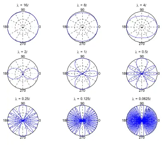
If the narrowband beamformer in Figure 2.2, with w = 1 and φ = 0, is

subject to signals over a large bandwidth the beamform will change considerably.

Figure 2.4 shows the directivity pattern changing drastically over a large

frequency range, with wavelengths from 16 to 1/16 times the distance between the

elements, in one octave steps. This range encompasses 9 octaves which is close to

the bandwidth of audio. The resulting beamforms range from nearly

omnidirectional to having 64 distinct lobes.

90

270

180 0

λ = 16l

90

270

180 0

λ = 8l

90

270

180 0

λ = 4l

90

270

180 0

λ = 2l

90

270

180 0

λ = 1l

90

270

180 0

λ = 0.5l

90

270

180 0

λ = 0.25l

90

270

180 0

λ = 0.125l

0.5 90

270

180 0

λ = 0.0625l

(13)

For broadband applications the desired directivity patterns remain the same

over the bandwidth, so systems of the general form shown in Figure 2.1 are no

longer useful. Past techniques used to help extend the bandwidth and improve the

beamforming performance of an array include weighting patterns fashioned after

binomial and chebeychev arithmetic schemes[4] and a method of synthesizing

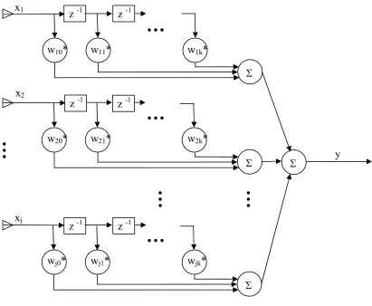
impulse functions[5]. A typical broadband beamformer of these types, shown in

Figure 2.5, uses a finite impulse response (FIR) filter on each sensor leg before the

summation. This provides the ability to change the gain and phase of the signals

differently for different frequencies. Like the narrowband case, the gains can be

fixed or adaptive. To accommodate the large audio bandwidth (approximately 10

octaves) the element spacing in the array must range from very small (at 20 kHz

where wavelength λ = 17 mm) to very large (at 20 Hz where λ = 17 m), so an

array would have to be very large and contain many elements to use this

technique. This large array size is impractical in may applications, so a search for

a new technique that will allow smaller array sizes (measured in physical

(14)

Figure 2.5. Typical Broadband Beamformer

Σ

x1

w20*

w10*

x2

xj

w11* w1k*

w21* w2k*

wj0*

z -1 z -1

wj1* wjk*

z -1

z -1 z -1

z -1

Σ

(15)

CHAPTER 3

TECHNIQUES

The initial purpose of this thesis was to develop a broadband array

processing technique for audio based on frequency up-conversion by mixing. This

technique is the first discussed in this chapter. The frequency up-conversion

technique did not produce the desired results so other techniques were developed

and studied. The final technique, based on group-delay discrimination, produced

exciting, useful results. This chapter describes each technique and its results.

3.1 Frequency Up-Conversion

3.1.1 Description

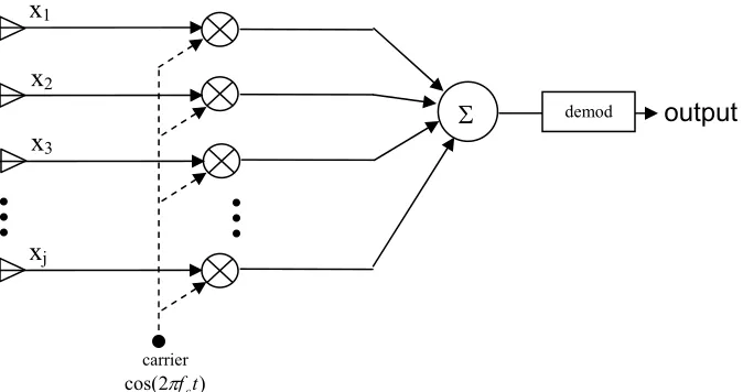
By mixing a base-band audio signal with a carrier signal much higher in

frequency, the bandwidth, in octaves, of the resulting spectrum is greatly reduced.

For example, a signal with frequency content from 20 Hz to 20 kHz,

approximately 10 octaves, is mixed with a carrier of 100 kHz. The resulting

spectrum is only 0.263 octaves wide (single sided), which appears to reduce the

effective variation in wavelength and thus decrease the effective spatial variation

of the signal being acquired. Can this be used to simplify the beamforming

problem by effectively reducing the bandwidth and possibly reducing the required

(16)

in the array by the same carrier before summation and demodulates after the

summation. Filtering the lower side-band created by the modulation and using a

chirp instead of a sinusoidal carrier are also considered.

3.1.2 Analysis

For an array of N elements letx

( )

t be the source signal, so x

(

t−τ_n

)

= − = N n n t x t y 1

τ cos(2πf_ct)y(t). Assuming an ideal demodulator the

output of the system is , the same output obtained for the simple case where

the received signals are only summed. This system is illustrated in figure 3.1.

( )

t

(17)

Figure 3.1. Frequency Up-Conversion Technique

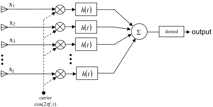
An attempt to make this scheme functional by further narrowing the

signal’s bandwidth was made using single side-band rather than the original dual

side-band modulation. Removing the lower side-band of each array element

signal after modulation with a filter described by impulse function yields

output e convolution, like multiplication, is

distributive the output similarly simplifies to .

Substituting , yields

( )

t h

(

)

(

)

[

∑

= ∗ − N n n ct x t ht f

1

) 2

cos( π τ

( )

]

and becaus

( )

(

)

_⎥ ⎦ ⎤ ⎢ ⎣ ⎡ − ∗

∑

= N n n ct x t f t h 1 ) 2

cos( π τ

( )

_∑

(

)

= − = N n n t x t y 1

τ h

( )

t ∗

[

cos(2πf_ct)y

( )

t

]

. Again, assuming an

ideal demodulator, the output of the system is y

( )

t , the same output obtained for

the simple case where the received signals are only summed. This single

side-band system is illustrated in figure 3.2.

(18)

Figure 3.2. Single Side-Band Frequency Up-Conversion Technique

A third attempt was made by modulating the signals with a chirp instead of

the sinusoidal carrier. The chirp technique suffers from the same problems as the

other frequency up-conversion techniques, and is therefore not discussed in further

detail.

3.1.3 Results

The resulting outputs of the modulated systems, when demodulated, are

nothing but the output obtained by simply summing the signals from the array

elements. This is due to the linear phase error characteristics of the mixing

process. For example, a 2 degree phase difference between elements at 100Hz,

still results in only a 2 degree phase shift at 100.1KHz after up-conversion. The

hope was that low frequencies in the band which did not create enough phase shift

Σ

x1

x2

x3

xj

output

demod

( )

t h

( )

t h

( )

t h

( )

t h

carrier

(19)

between receiving elements due to the long wavelengths, would experience a

larger phase shift after up-conversion. This was not the case.

3.2 Non-Linear Decimation

3.2.1 Description

The non-linear decimation approach is centered on the concept of reducing

the effective wavelength of a signal by removing samples in the time domain

sequence. This is predicated first by the assumption that the signal is oversampled

such that after decimation, the bandwidth is still usable. This approach is

described in continuous time by the time scaling property of the Fourier transform

⎟ ⎠ ⎞ ⎜ ⎝ ⎛ ⇒

a f X a at

x( ) 1

where a is a real nonzero constant. If oversampling is not achieved, the problem

becomes more than just a scaling operation and there can be a loss of information

through aliasing.

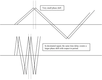
Given there is a constant time delay for a given angle between receiving

elements, that time delay will manifest itself as a phase difference. However, due

to the geometry of the elements, that phase difference can be negligible at very

long wavelengths. By keeping the delay the same but decimating the time

(20)

In decimated signal, the same time delay creates a larger phase shift with respect to period. Very small phase shift

Figure 3.3 Decimation in Time

However, in order to accomplish this, there are three critical issues that are

“showstoppers” for using this technique.

3.2.2 Analysis

First, there is no reduced scaling of the bandwidth with respect to octaves

traversed. Section 3.1 shows how an up-conversion process could effectively

reduce the relative octaves in the signal from 10 octaves to 0.263 octaves and still

maintain a 20 Khz bandwidth. When linearly decimating the signal, the frequency

(21)

reduction in octaves and there will be no improvement of the spatial variation of

the array vs. frequency. This is best seen with a simple example using a square

wave. A 100 Hz square wave with 50% duty cycle will have the following

harmonics present: 100Hz, 300 Hz, 500Hz, 700Hz, 900Hz, etc. If the signal is

sufficiently oversampled, and the samples are reduced by a factor of 10, the period

is now 1/10 of what it was. The result is a square wave with a fundamental

frequency of 1 KHz which contains harmonics equal to 3 KHz, 5 KHz, 7 KHz, 9

KHz, etc. The bandwidth has shifted up in frequency by a factor of 10, and more

importantly, the bandwidth occupies over 3 octaves in both signals. There is no

change.

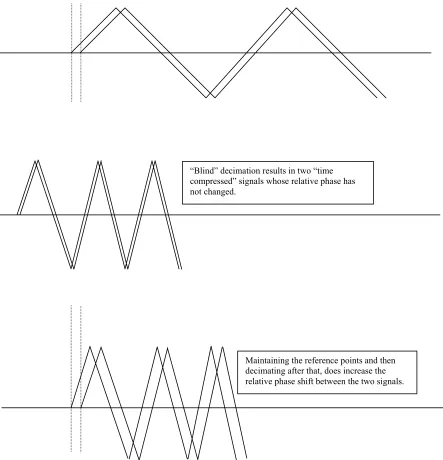
Secondly, in order to use decimation to effectively increase the phase

difference at long wavelengths, a non-linear process must be implemented.

Blindly decimating both receiver signals does not increase the phase shift between

the two receivers. Instead, a threshold must be set to mark the original position in

time of the two signals and this position must be maintained. Without “moving”

the signals from their original positions, the signals are then decimated from the

(22)

“Blind” decimation results in two “time compressed” signals whose relative phase has not changed.

Maintaining the reference points and then decimating after that, does increase the relative phase shift between the two signals.

(23)

Lastly, this technique only considers one incoming signal. If more than one

spatially separated, simultaneous signal is present, the algorithm breaks down.

Because the reference marking algorithm would have to be based on received

signal amplitude and the superposition of more than one signal causes amplitude

distortion, reference marking would be unreliable. Hence, the implementation of

this in a working environment such as the theater becomes unrealistic. It will be

found to be much easier to differentiate simultaneous signals by their magnitude

and phase responses in the frequency domain.

3.3 Group Delay Discrimination

3.3.1 Description

This technique uses the difference in group delay of the signals from two

array elements to produce a temporal filter which masks frequencies contained in

any off-axis interference. The filter is then applied to the signal from one element

to produce the output. The filter is determined by first finding the Fourier

transforms of the signals from the two array elements and expressing the

transforms as a magnitude and a phase. Because the processing will be performed

digitally, the discrete Fourier transform (DFT) is considered here. The forward

DFT is given by

( )

∑

−

( )

=

− = 1

0

2

N

n

N kn j e n x k

X

π

and the inverse by

( )

∑

−

( )

= = 1

0

2 1 N

k

N kn j e k X N n x

π .

(24)

from the phase of the transforms through differentiation with respect to angular

frequency. Group delay is usually defined as the negative derivative of phase with

respect to angular frequency ω φ

d d

− where φ =∠X

( )

ω [6]. The technique described

in this chapter does not require that the group delay be the negative derivative, so

group delay can be redefined here as

ω φ ω τ

d d

=

)

( . Because the system is discrete,

an approximation of the derivative must be used. Once the group delays for the

signals at each element are calculated, their difference is determined and used to

define the filter’s transfer function (determining the filter’s transfer function is

discussed in the next section). Applying the filter to the signal from either array

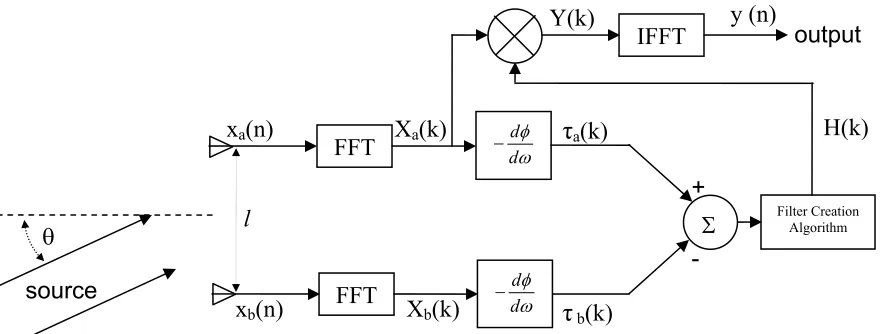
element masks the frequency content not arriving on axis. The process is outlined

in figure 3.5 and the algorithm is discussed in detail in section 3.3.2.

A technique is used in radar applications where a number of return signals

are processed by two or more antenna elements, and “tagged” or characterized by

their phase (incident angle) and frequency. Then an algorithm can decide which

signals to prioritize and which signals to throw out if any. The similarities have to

do with having the ability to determine from what direction signals of different

(25)

Figure 3.5. Group Delay Discrimination Process

3.3.2 Analysis

For a signal arriving at a two element array, the time delay between

elements is a function of the incident angle θ and is described by the equation

c l θ

τ = sin , where c is the propagation speed. The phase difference between the

two elements is a function of the angle of propagation and frequency of the signal

and is described by the equation

c l

f θ

π

φ = 2 sin . Taking the derivative of φ with

respect to angular frequencyω =2π f gives θ τ ω φ = = c l d d sin

, the time delay shown

above. This is the group delay of the signal, and can be used to determine the

incident angle of a received signal. If more than one signal from different

directions are present, the group delay, because it is a function of frequency, can

show the direction from which the signals are coming if the frequency content of

Σ θ source output l FFT FFT xa(n)

xb(n)

Xa(k)

Xb(k)

ω φ d d − + - τa(k)

τb(k)

Filter Creation Algorithm

H(k) IFFT

Y(k) y (n)

ω φ

d d

(26)

There are three instances where cyclic phenomenon must be considered.

The first is where there can be more than half of one complete wavelength of a

waveform within the spacing of the array elements. The difference in phase of the

waveforms at the elements is cyclic. Consider two sinusoids of the same

frequency with different phase. If the phase difference between the two signals is

smaller than π, no problem is encountered. Because the interest here is in the

absolute phase difference between the signals and a leading or lagging relationship

cannot be discerned, differences of π or more may cause problems. For example,

a phase difference of 1.5π can be said to be separated by 1.5π or 0.5π. This can

cause interference to masquerade as a desired signal. This problem is remedied by

spacing the array elements a distance smaller than half of the smallest wavelength

in the band. Placing the array elements (remember there are only two) extremely

close together may limit the ability of the beamformer to notice a phase difference

in signals with large wavelengths. This can be overcome by using more than two

elements and letting the closely spaced elements handle the small wavelengths and

the distantly spaced elements handle the large wavelengths.

The second cyclic problem also has to do with the phase of the incoming

signals before the difference. This is when the phase values of a signal (not the

difference in phase) wrap around as frequency increases. For instance, if the

phase values of a signal at adjacent frequency samples are 0.2π apart with values

(27)

in Matlab. The unwrap function removes the phase discontinuities by adding or

subtracting appropriate multiples of 2π. For example the sequence

[

0.8π 0.9π −π −0.9π

]

unwraps to

[

0.8π 0.9π π 1.1π

]

.

The third instance of possible problem causing cyclic phenomenon has to

do with the recursive nature of the DFT and the length of the signal being

processed. As far as the DFT is concerned, signals in both domains repeat

indefinitely in both directions. For instance, the time-domain sequence of four

samples

[

( )

1 0 0 0

]

is actually

[

_L 1 0 0 0

( )

1 0 0 0 1 0 0 0 _L

]

,

so when comparing two signals it may not be clear what the time delay between

them is. For example, the two sequences

( )

⎥ ⎦ ⎤ ⎢ ⎣ ⎡ L L L L 1 0 0 0 1 0 0 0 0 0 0 1 0 0 0 1 1 0 0 0 0 0 0 1

are cyclic. The impulses could be said to be separated by one or three samples,

depending on which sequence is used as the reference. This type of ambiguity can

be remedied by padding sequences of N samples with N zeros or assuring that

delays of more than half of the sequence length are not possible. Zero padding the

two sequences above gives the following:

⎥ ⎦ ⎤ ⎢ ⎣ ⎡ L L L L 0 0 0 0 0 0 0 0 0 0 0 0 0 0 0 0 1 0 0 0 ) ( 1 0 0 0 0 0 0 1 ) ( 0 0 0 1 0 0 0 0 0 0 0 0 1 0 0 0 0 0 0 1

The zero padding ensures that the minimum distance between impulses is the

(28)

3.3.3 Implementation

In the first step of the algorithm, the received time domain signals are zero

k , the phases, ∠X_a

( )

k

and , are determined. Next the group delay is to be calculated. The

approximate derivative can then be calculated. (In the actual implementation, the

difference in phase is calculated, and the group delay calculation is performed on

this difference; mathematically the processes are the same, but performing only

one approximate derivative makes the process more efficient.) The approximate

derivative used in the calculation is simply the difference between adjacent points

which leaves a vector with one less sample than the input. This is because the

values of the approximate derivative actually fall between the discrete frequency

samples of the signal. This presents a problem when doing further calculations,

but the difference between the first and last points of the phase can be substituted

for the “missing” sample. Placing this “extra” sample before or after the N-1

difference will dictate whether the approximate derivative is a forward or

backward difference. Either can be used. The group delay difference is then fed

into the filter creation algorithm.

( )

k

X_b

(29)

The filter creation algorithm uses the group delay difference to determine

what frequencies are wanted and which are not. A filter, H(k), is created to

remove those frequencies which are not wanted. Where the group delay

difference is zero, the signal is arriving at the two elements at the same time,

which indicates that the signal is arriving on axis (perpendicular to the line defined

by the two array elements). The on axis signals are wanted; all others are not. For

the calculated group delay difference, a function of frequency is created to be

unity when the group delay difference is close to zero (wanted signal) and zero

otherwise (unwanted signal), and the function is used as the filter.

max max

) ( 0

) ( 1

) (

τ τ

> ≤ =

f for

f for f

H

The parameter τmaxis calculated with the formula

c l _max

max

sinθ

τ = based on the

desired maximum angle of the beamformθ_max. The directivity pattern will ideally

be one between −θmax and θmax and zero otherwise. The filter creation algorithm

described is certainly not the only method that can be used. Any function of the

group delay difference may be used to produce other beamforms.

The filter is then applied to the signal from one of the elements. Because

the filter is described by its transfer function and the Fourier transform of the

incoming signal has been determined, the filter is implemented my multiplication

(30)

performed and the result is truncated (because of the zero padding in the first step)

yielding the output of the system y(n).

This technique can be implemented in near real time if small adjacent time

frames are processed serially. The number of samples should be large enough to

have adequate resolution in the frequency domain.

3.3.4 Results

The algorithm was implemented in MATLAB and first tested with the

following parameters:

Sampling Frequency fs= 8 Hz

Number of Samples N = 4 Element Spacing l = 1

Maximum Incident Angle ₁₀_.₈o

max = θ Propagation Speed c = 1

One incoming signal is considered; it is a discrete impulse .

Four incident angles

( )

[

1 0 0 0

]

θ are considered which are , , , and

. The angles are chosen to create delays of 0, 1, 2, and 3 samples

respectively. The maximum incident angle corresponds to a time

delay which falls between 2 and 3 samples. Therefore, the incident angles

and should return the signal and the incident angles

and should reject the signal. For each of the four incident angles

o

0

=

θ _θ ₌₇_.₁₈o _θ ₌₁₄_.₄₇₇o

o

024 . 22

=

θ

o

8 . 10 max = θ

o

0

=

θ θ ₌₇_.₁₈o θ ₌₁₄_.₄₇₇o

o

024 . 22

=

θ θ, a

step by step walkthrough of the algorithm is shown.

(31)

Incoming signal x =

[

( )

1 0 0 0

[

1 0 0 0 0 0 0 0

]

= bp x

Performing the FFT

( )

[

1 1 1 1 1 1 1 1

]

= ap X

( )

[

1 1 1 1 1 1 1 1

]

0 1 0 0

]

= b x

Padding with N zeros

( )

[

1 0 0 0 0 0 0 0

]

= ap x

( )

[

0 1 0 0 0 0 0 0

]

= bp x

Performing the FFT

( )

[

1 1 1 1 1 1 1 1

]

= ap X

( ) (

)

(

)

(

)

(

)

_⎥ ⎦ ⎤ ⎢ ⎣ ⎡ − ₋ − − ₋ − + + = 2 1 1 1 2 1 1 1 2 1 1 1 2 1 1

1 j j j j j j

X_bp

( )

[

0 0 0 0 0 0 0 0

]

= ∠X_ap

( )

_⎥⎦⎤ ⎢⎣ ⎡ ₋ ₋ ₋ ₋ ₋ ₋ ₋ = ∠ 4 7 2 3 4 5 4 3 2 4

0 π π π π π π π

bp X

( )

_⎥⎦⎤ ⎢⎣ ⎡ = ∠ − ∠ 4 7 2 3 4 5 4 3 2 4

bp

ap X

X

Calculating the group delay difference ⎥⎦ ⎤ ⎢⎣ ⎡ = 8 1 8 1 8 1 8 1 8 1 8 1 8 1 8 1 1 τ

Creating the filter

[

1 1 1 1 1 1 1 1

]

= H

( )

[

1 1 1 1 1 1 1 1

]

= = × _p ap H Y X

Performing the IFFT

( )

[

1 0 0 0 0 0 0 0

]

= p y

( )

]

]

= ∠X_ap

( )

_⎥⎦⎤ ⎢⎣ ⎡ ₋ ₋ ₋ ₋ ₋ ₋ ₋ = ∠ 2 7 3 2 5 2 2 3 2

bp X

( )

_⎥⎦⎤ ⎢⎣ ⎡ = ∠ − ∠ 2 7 3 2 5 2 2 3 2

bp

ap X

X

Calculating the group delay difference

⎥⎦ ⎤ ⎢⎣ ⎡ = 4 1 4 1 4 1 4 1 4 1 4 1 4 1 4 1 1 τ

Creating the filter

[

= p y

( )

[

0 0 0 0

]

]

= bp x

Performing the FFT

( )

[

1 1 1 1 1 1 1 1

]

= ap X

( ) (

)

(

)

(

)

(

)

_⎥ ⎦ ⎤ ⎢ ⎣ ⎡ − − − ₋ + ₋ − + = 2 1 1 1 2 1 1 1 2 1 1 1 2 1 1

1 j j j j j j

X_bp

( )

[

0 0 0 0 0 0 0 0

]

= ∠X_ap

( )

_⎥⎦⎤ ⎢⎣ ⎡ ₋ ₋ ₋ ₋ ₋ ₋ ₋ = ∠ 4 21 2 9 4 15 3 4 9 2 3 4 3

bp X

( )

_⎥⎦⎤ ⎢⎣ ⎡ = ∠ − ∠ 4 21 2 9 4 15 3 4 9 2 3 4 3

bp

ap X

X

Calculating the group delay difference ⎥⎦ ⎤ ⎢⎣ ⎡ = 8 3 8 3 8 3 8 3 8 3 8 3 8 3 8 3 1 τ

Creating the filter

[

= p y

( )

[

0 0 0 0

]

(35)

The previous example shows that for one simple broadband signal the

algorithm successfully returns the signal if it is within the specified pattern and

removes it if not.

The algorithm was then tested with recorded audio vocal data and a square

wave. The system parameters are:

Sampling Frequency fs= 44.1 kHz

Frame Size N = 2205 samples (50 ms)

Element Spacing l = .05 m

Maximum Incident Angle ₁₀o

max = θ

Propagation Speed c = 340.29 m/s

The signals are 2 seconds long and are processed in N length sequential

frames. Zero padding is not used because the maximum time delay between the

elements ( =0.147

c l

milliseconds) is less than half of the frame size (50

milliseconds). The test signals are a 300 Hz, 50% duty cycle square wave with an

amplitude of 1 (square300.wav) and a vocal sample “Now we are about to reach

the end of the road”(end_of_the_road.wav). The signals used are 2 seconds in

(36)

Figure 3.6. Frequency Content of Group Delay Algorithm Test Signals

The first test has the square wave arriving at zero angle of incidence. The

algorithm should produce the square wave unaltered. The difference between the

output and the input is on the order of . The error is caused by rounding

errors in the FFT/IFFT calculations. If the FFT and IFFT of the square wave are

performed sequentially for the 50 ms frames, the error is identical to the error

produced by the algorithm.

(37)

The second test has the square wave arriving at an angle of incidence of 30

degrees. The desired output here is zero. The actual output is a tone at 14.7 KHz

which is the 49th harmonic of the 300 Hz square wave. The amplitude is 0.0204

which is the same as the amplitude of this harmonic of the square wave. This

harmonic passes through the algorithm untouched because the element spacing is

too large to guarantee that more than one half of a cycle of the incoming signal at

14.7 KHz can span the elements. This was expected.

The third test has the vocal sample “Now we are about to reach the end of

the road.” arriving at zero angle of incidence. The algorithm should produce the

unaltered sample. The difference between the output and the input is on the order

of . The error is caused by rounding errors in the FFT/IFFT calculations, as

in test one. If the FFT and IFFT of the test signal are performed sequentially for

the 50 ms frames, the error is identical to the error produced by the algorithm.

16 10−

The fourth test has the vocal sample “Now we are about to reach the end of

the road.” arriving at an angle of incidence of 30 degrees. The desired output here,

as in the square wave case (Test 2), is zero. The algorithm does not completely

eliminate the signal and creates many artifacts from the process. This can be

explained by the unwrap function not being able to cope with rapidly changing

phase values over frequency for each incoming signal. Large changes in phase

may actually be different by factors of 2π or greater, but the unwrap function

(38)

algorithm will let the corresponding frequency content through. The output can be

heard in ‘Test4_output.wav’

Figure 3.7. Test 4 Input and Output Comparison

Up until this point only single sources have been used in the tests. The fifth

test will simulate a wanted source and interference arriving simultaneously. The

vocal sample “Now we are about to reach the end of the road.” is arriving at zero

angle of incidence and the square wave is arriving at an angle of incidence of 30

(39)

‘Test5_input.wav’. The vocal sample is unintelligible because it is “buried” under

the square wave. The algorithm should return the vocal sample and remove the

square wave except where the frequency content overlaps. The actual output of

the system can be heard in ‘Test5_output.wav’ and shows the power of the

algorithm to remove interference. The vocal sample can be heard clearly with

only the harmonic of the square wave at 14.7 kHz (as in Test 2) and a few artifacts

from processing of the signal in frames.

(40)

CHAPTER 4

CONCLUSIONS

The first two techniques discussed (Frequency Up-Conversion and

Non-Linear Decimation) do not prove to be useful in solving any of the problems

associated with broadband beamforming, but the work done on them did provide a

better understanding of the goings on in beamforming arrays. This understanding

led to the design of the group delay discrimination technique.

The group delay discrimination technique meets the proposed goals by

using an array much smaller (in physical size and number of elements) than

traditional broadband beamforming techniques and the directivity pattern stays

constant over bandwidth (if the frequency content of the signals do not overlap).

In order to meet these goals, tradeoffs were made in the types of signals that can

be acquired. The tradeoffs are that the frequency content of the signals cannot

overlap and the phase of the signals does not change too rapidly for the algorithm

to handle. If the phase discontinuity problem can be resolved, the algorithm may

still work well for many of the intended applications if the frequency content of

the interference does not mostly mask the frequency content of the wanted signal.

If two speakers (one wanted and one unwanted) have different voice profiles the

(41)

The group delay discrimination technique can be improved and expanded upon

by further research into:

• Using an improved algorithm to “unwrap” the phase information.

• Processing more than two sensors for larger bandwidth performance.

• Processing more than two sensors for three dimensional pickup patterns.

• Improving the filter creation algorithm to create more complex beamforms.

Further research into the uses of the group delay discrimination technique

can include but is certainly not limited to direction finding and source localization

for both acoustic and electromagnetic sources. The group delay discrimination

algorithm was developed for use in audio-band acoustics, but like beamforming in

general, it can be applied to a number of different fields and is certainly not

(42)

REFERENCES

[1] Klapholz J., “The History and Development of Microphones,” Sound &

Communications magazine, September 1986

[2] Van Veen, B. D. & Buckley, K. M., “Beamforming: A Versitile Approach to Spatial Filtering,” IEEE Accoustics, Speech, and Signal Processing Magizine, vol. 5(2), pp. 4-24, April 1998.

[3] Widrow, B. & Stearns, S. D., “Adaptive Signal Processing,” Prentice Hall, 1985.

[4] Balanis, C. A., “Antenna Theory” John Wiley & Sons, Inc, 1982.

[5] Lannes, K. J., “Improvements of Phased Array Performnce by the Use of Synthesizing Impulse Functions,” Masters Thesis,University of Texas at Arlington Libraries, 1994

(43)

APPENDIX

Audio Files from Group Delay Discrimination Testing:

‘square300.wav’

‘end_of_the_road.wav’

‘TEST4_output.wav’

‘TEST5_input.wav’

‘TEST5_output.wav’

Matlab Function which Performs Grpup Delay Discrimination Algorithm:

(44)

VITA

Ryan Thiel was born in 1978 in New Orleans, LA. He studied Electrical