Issues
ISSN: 2146-4138
available at http: www.econjournals.com
International Journal of Economics and Financial Issues, 2020, 10(1), 59-66.
Investment Performance of Machine Learning: Analysis of S&P
500 Index
Chia-Cheng Chen
1, Chun-Hung Chen
2, Ting-Yin Liu
3*
1Department of Finance, Ling Tung University of Science and Technology, Taichung, Taiwan, 2Department of Finance, National Yunlin University of Science and Technology, Doulium, Yunlin County, Taiwan, 3Department of Business Affairs, Mingdao High School, Taichung, Taiwan. *Email: [email protected]
Received: 02 October 2019 Accepted: 05 December 2019 DOI: https://doi.org/10.32479/ijefi.8925
ABSTRACT
This study aims to explore the prediction of S&P 500 stock price movement and conduct an analysis of its investment performance. Based on the S&P
500 index, the study compares three machine learning models: Artificial neural networks (ANN), support vector machines (SVM), and random forest. With a performance evaluation of S&P 500 index historical data spanning from 2014 to 2018, we find: (1) By overall performance measures, machine learning models outperform benchmark market index. (2) By risk-adjusted measures, the empirical results suggest that Random Forest generates the
best performance, followed by SVM and ANN.
Keywords: Artificial Neural Network, Support Vector Machines, Random Forest, Machine Learning, Investment Performance
JEL Classifications: C11, C15, C53, G17
1. INTRODUCTION
In recent years, deep learning, machine learning, and artificial intelligence (AI) are mainstream. Despite the fact that there have
been a number of empirical researches conducted on machine
learning to predict share price movement (Ciner, 2019; Du, 2018; Long et al., 2019; Hiransha et al., 2018; Yang et al., 2019), attention has been paid majorly to the prediction efficacy of machine
learning rather and little on the aspects of performance and risk
measurement. Therefore, this study aims to fill the gap and delve into the financial evaluation of machine learning applications in
the S&P 500.
Stock market price movement prediction has to confront the
strongest rejection from the academic paradigm of efficient market hypothesis states that prices of stocks are informationally efficient
which means that it is impossible to predict stock prices based on
the trading data (Malkiel and Fama, 1970). However, more recent
results show that, if the information obtained from stock prices is
pre-processed efficiently and appropriate algorithms are applied
then the trend of stock or stock price index may be predictable
(Patel et al., 2015). The new discovery can greatly benefit market
practitioners because accurate predictions of the movement of stock price indexes are very important for developing effective
market trading strategies (Leung et al., 2000).
The main objective of the research is to input the results of
ten technical analysis indicators into artificial neural networks (ANN), support vector machines (SVM), and Random Forest
models to predict stock price movement and evaluate investment performance and risk measurement. In the circumstance, the machine learning models buy stocks when predicting a rise and short stocks when predicting a decline in prices. Based on
the S&P 500 (GSPC) Index from 2014 to 2018, this research
compares the investment performance among the machine learning models.
The remainder of this paper are organized as follows. Section 2 provides a brief overview of the theoretical literature. Section 3 describes the research data. Section 4 provides the prediction models and risk-adjusted measures used in this study. Section 5 reports the empirical results from the comparative analysis. Finally, Section 6 contains the concluding remarks.
2. LITERATURE REVIEW
For a long time, it was impossible that changes in the prices of stocks can be forecastable. Predicting returns in the stock market is usually posed as a forecasting problem where prices are predicted. Intrinsic volatility in the stock market across the globe makes the task of prediction challenging. Stock prediction and selection have
long been identified as an important but challenging topic in the research area of financial market analysis (Du, 2018; Henrique et al., 2019; Long et al., 2019). In this section, we focus the review
of previous studies on ANN, SVM, and random forest applied to stock market prediction and investment performance.
To quest the future features of stock markets, various forecasting
algorithms have been employed, of which, computational
intelligence (CI) (or AI) has become increasingly dominant due
to its powerful learning capability and high prediction accuracy.
Typical CI techniques in stock market prediction (for stock prices, stock returns, market indexes, etc.) are ANNs (Du, 2018; Kim and Shin, 2007; Qiu et al., 2016; Xi et al., 2014) and SVMs (Kazem et al., 2013; Li et al., 2014; Li et al., 2015; Yang et al., 2019).
ANN and SVM have been demonstrated to provide promising
results in predict the stock price return (Henrique et al., 2019; Huang and Liu, 2019; Kara et al., 2011; Khan et al., 2016; Patel et al., 2015; Zhang et al., 2019). Hassan et al. (2007) propose
and implement a fusion model by combining the Hidden Markov
Model (HMM), ANN and Genetic Algorithms (GA) to forecast financial market behavior. Using ANN, the daily stock prices
are transformed into independent sets of values that become an input to HMM. Forecasts are obtained for a number of securities in the IT sector and are compared with a conventional forecast method.
Wang et al. (2016) are developed and combined a hybrid v-support vector regression (SVR) model with principal component analysis
and brainstorm optimization for stock price index forecasting. Numerical results indicate that the developed hybrid model is not only simple but also able to satisfactorily approximate the actual CSI300stock price index, and it can be an effective tool in stock
market mining and analysis. Yang et al. (2019) predict stock market price with a forecasting model based on chaotic mapping, firefly algorithm, and SVR. Compared with genetic algorithm-based SVR (SVR-GA), chaotic genetic algorithm-based SVR (SVR-CGA), firefly-based SVR (SVR-FA), ANNs and adaptive neuro-fuzzy
inference systems, the proposed model performs best based on
two error measures, namely mean squared error and mean absolute
percent error.
Gupta et al. (2018) use quantile random forests to study the
predictive value of various consumption-based and
income-based inequality measures across the quantiles of the conditional distribution of stock returns. Results suggest that the inequality
measures have predictive value for stock returns in sample, but do not systematically predict stock returns out of the sample.
Ciner (2019) show that when the random forest method, which
accounts for both linear and nonlinear dynamics, is used for
regression, industry returns indeed contain significant out of
sample forecasting power for the market index return. Basak
et al. (2018) develop an experimental framework for the classification problem which predicts whether stock prices will
increase or decrease with respect to the price prevailing n days
earlier. Two algorithms, Random Forests, and gradient boosted
decision trees facilitate this connection by using ensembles of decision trees.
Khan et al. (2016) employ several algorithms in stock prediction
such as SVM, ANN, linear discriminant analysis, linear regression,
K-NN, and Naïve Bayesian Classifier to approach the subject of predictability with greater accuracy. Chatzis et al. (2018) leverage the merits of a series of techniques including classification
trees, SVM, random forests, neural networks, extreme gradient
boosting, and deep neural networks and find significant evidence
of interdependence and cross-contagion effects among stock, bond and currency markets.
3. RESEARCH DATA
The data used in this paper all come from yahoo finance (https:// finance.yahoo.com/). We collect 1258 S&P 500 (GSPC) Index samples from the yahoo finance over January 2014 to December
2018 period. These data form our entire data set. Percentage-wise increase and decrease cases of each year in the entire data set are shown in Table 1.
There are some technical indicators through which one can predict the future movement of stocks. Here in this study, a total of ten
technical indicators as employed in Kara et al. (2011) are used.
These indicators are shown in Table 2.
In the research, we input the results of ten technical analysis
indicators into ANN, SVM and Random Forest models to predict
stock price movement. In the circumstance in which the transaction costs are calculated, the machine learning models buy stocks when predicting a rise and short stocks when predicting a decline
in prices. Based on the S&P 500 (GSPC) Index, the research compares the investment efficiency between the machine learning
models.
Table 1: The number of increase and decrease cases percentage in each year in the entire data set of the S&P 500 index
Year Increase % Decrease % Total
2014 144 57 108 43 252
2015 119 47 133 53 252
2016 132 52 120 48 252
2017 143 57 108 43 251
2018 132 53 119 47 251
4. PREDICTION MODELS AND
RISK-ADJUSTED MEASURES
4.1. Prediction Models
4.1.1. ANN
The ANNs are non-linear models that make use of a structure capable to represent arbitrary complex non-linear processes that
relate the inputs and outputs of any system (Chatzis et al., 2018; Chen et al., 2003; Hassan et al., 2007; Henrique et al., 2019; Huang and Liu, 2019; Kara et al., 2011; Khan et al., 2016; Leung et al., 2000; Olson and Mossman, 2003; Patel et al., 2015). ANN represents one widely used soft computing technique for stock market forecasting. ANN has demonstrated capability in financial modeling and prediction (Huang and Liu, 2019; Kara et al., 2011; Leung et al., 2000; Olson and Mossman, 2003; Patel et al., 2015).
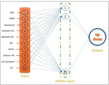
In this study, a three-layered feedforward ANN model was structured to predict the stock price index movement. This ANN model consists of an input layer, a hidden layer and an output layer, each of which is connected to the other. The ANN architecture is
defined by the way in which the neurons are interconnected. The
network is fed with a set of input-output pairs and is trained to
reproduce the output. The number of neurons (hn) in the hidden layer, the value of learning rate (lr), momentum constant (mc) and the number of iterations (ep) are ANN model parameters
that must be efficiently determined. Inputs for the network were
ten technical indicators that were represented by ten neurons in the input layer. The architecture of the three-layered feedforward ANN is illustrated in Figure 1. The investment performance of ANN prediction model are summarized in Table 3.
4.1.2. SVM
In machine learning, SVM are supervised learning models with associated learning algorithms that analyze data used for
classification and regression analysis. SVM emerged from research
in statistical learning theory on how to regulate generalization
and find an optimal trade-off between structural complexity and
empirical risk. SVMs classify points by assigning them to one of two disjoint half-spaces, either in the pattern space or in a higher-dimensional feature space. One of the most popular SVM
classifiers is the “maximum margin” one, which aims to minimize
an upper bound on the generalization error through maximizing
the margin between two disjoint half-planes (Burges, 1998; Cortes and Vapnik, 1995; Patel et al., 2015). A SVM is a discriminative classifier formally defined by a separating hyperplane. In other words, given labeled training data (supervised learning), the
algorithm outputs an optimal hyperplane which categorizes new examples. In two dimensional space, this hyperplane is a line dividing a plane into two parts wherein each class lay on either
side (Bhatia and Madaan, 2018).
The main idea of a SVM is to construct a hyperplane as the decision surface such that the margin of separation between positive and
negative examples is maximized (Xu et al., 2009). The equation
of the hyperplane can be given as:
ωT+b=0 (1)
The margin is width is 2/‖ω‖ and the learning problem is equivalent
to unconstrained optimization problem over ω.
min2
0 1
+C
∑
y −y f xi iN
max( , ( )) (2)
SVM are highly effective in high dimensional spaces but under
perform when target classes (for classification problems) are
overlapping i.e. kernel functions need to be used.
The architecture of SVM is illustrated in Figure 2. The investment performance of SVM prediction model is summarized in Table 3.
4.1.3. Random forest
Random Forest is an ensemble, data-miner which uses “deep” (unpruned) decision trees as base learners. It is a modification of applying to bag to multiple classifications and regression trees,
and averaging the predictions of the approximately uncorrelated
trees to yield the final estimate. Random Forest model was
unable to show any clear patterns in the data through variable
importance plots and did not show any significant improvement in performance in comparison to generalized linear models (Bhatia and Madaan, 2018). Decision tree learning is one of the most popular techniques for classification. Its classification accuracy is comparable with other classification methods, and it is very efficient.
Table 2: Selected technical indicators and their formulas
Name of
indicators Formulas
SMA (10-day) C Ct+ t−1+ +Ct−9
10
WMA (10-day) (( ) ( ) )
( )
n C n C C
n n
t t t
× + − × + +
+ −
(
)
+ +− −1
1 1
1 9
Momentum Ct−Ct−n
Stochastic K% C LL
HHtt n LLt nt n
− − − × − − 100 Stochastic D% i n t i K n = − −
∑
0 1 % Relative strengthindex (RSI) 100 100
1 0 1 0 1 − +
(
=− −) (
=)
− −∑
i∑
n
t i i
n t i
Up /n / Dw /n
MACD
MACD n
n DIFF MACD n
t t t
( )− + ( ( )−) + × − 1 1 2 1 Larry William’s
R% HHn CLt
n n
−
− ×100
A/D oscillator H C
Htt Ltt
−
− −1
Commodity channel index (CCI) M SM D t t t −
0 015.
Ct is the closing price, Lt is the low price, Ht is the high price at time t, DIFFt=EMA
(12) t−EMA (26) t, EMA is exponential moving average, EMA(k) t=EMA(k) t−1+α×
(Ct−EMA(k) t−1), α is a smoothing factor, α= +
2 1
k , k is time period of k day exponential moving average, LLt and HHtmean lowest low and highest high in the last t days,
respectively. Mt=Ht+L Ct+ t 3 , SM
M n t i n t i
=
(
∑=1 − +1)
,D M SM
n
t i n
t i t
=
(
∑=1| − +1− |)
, UP tRandom forests or random decision forests are an ensemble learning method for classification, regression and other tasks
that operates by constructing a multitude of decision trees at training time and outputting the class that is the mode of the
classification. It uses decision tree as the base learner of the ensemble. The idea of ensemble learning is that a single classifier is not sufficient for determining class of test data. Reason being, based on sample data, classifier is not able to distinguish between
noise and pattern. So it performs sampling with replacement such that given n trees to be learnt are based on these data set samples. After creation of n trees, when testing data is used, the decision which majority of trees come up with is considered as
the final output. This also avoids problem of over-fitting. The
investment performance of random forests prediction model is summarized in Table 3.
5. EXPERIMENTAL RESULTS AND
ANALYSIS
The research empirically examines the financial performance
of machine learning through performance measures, such as Jensen’s Alpha, Sharpe ratio, Treynor ratio, information ratio, and Modigliani ratio. Our experimental results are based on data
retrieved from the S&P 500 Index (from 2014 to 2018). The empirical results are presented firstly by descriptive statistics,
followed by an annual evaluation analysis, and concluded with overall performance comparison among machine learning models.
5.1. Descriptive Statistics
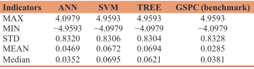
The analysis of the overall performance of ANN, SVM, and
Random Forest models is undertaken base on the benchmarks indices, the S&P 500 Index (GSPC). The descriptive statistics
of the daily returns for the benchmark indices, and for the three machine learning models are reported in Table 4. Figure 3 is the daily return chart of machine learning models and GSPC from 2014 to 2018.
Figure 1: Architecture of artificial neural networks
Table 3: Annual returns of three prediction model with benchmark
Prediction
models 2014 2015 2016 2017 2018 5 years
GSPC
(Benchmark) 12.28 −1.03 12.34 17.95 −5.69 35.85
ANN −7.00 28.81 9.09 2.29 25.87 59.06
SVM 25.91 4.54 17.49 22.71 13.90 84.55
Random
forest 25.31 31.96 15.11 24.12 −9.14 87.36
ANN is the artificial neural network, SVM is the support vector machines, TREE is the
As presented in Table 4 and Figure 3, our proposed machine
learning models generate significantly higher mean returns. In
terms of average daily return, SVM and random forest generate
2 times higher returns than GSPC (benchmark); with ANN of
1.5 times. Among the machine learning models, the results indicate that the order of investment performance excellence can be put down as follows: SVM, random forest, and ANN.
For the entire sample period, the cumulative returns of ANN,
SVM, and Random Forest are respectively of 59.06%, 84.55%, and 87.36% in Figure 4. By annual data, our machine learning models
are particularly impressive during the bear markets. Specifically, in 2015 with a market return of −1.03%, ANN, SVM, and random forest are respectively of 28.81%, 4.54%, and 31.96%. Likewise, in 2018 with a market return of −5.69%, ANN and SVM are
respectively of 25.87% and 13.90%. Overall, our empirical results
suggest machine learning is promising for higher cumulative returns in the S&P 500 index applications.
5.2. Risk-adjusted Measures
5.2.1. Sharpe ratio
The Sharpe ratio is used to help investors understand the return of an investment compared to its risk. The ratio is the average return earned in excess of the risk-free rate per unit of volatility or total risk. Subtracting the risk-free rate from the mean return
allows an investor to better isolate the profits associated with
risk-taking activities. Generally, the greater the value of the Sharpe ratio, the more attractive the risk-adjusted return. In
particular, a negative Sharpe ratio indicates a situation of “anti-skill,” since the performance of the riskless asset is clearly
superior.
According to Table 5, it is evident from the empirical results presented in proposed machine learning models outperform the
benchmark. More specifically, the Sharpe ratios of GSPC in 2015
and 2018 produce negative values, indicating no investment worth. The Sharpe ratios of ANN, SVM, and random forest are almost positive for all 5 years and outperform that of GSPC. In short, the
Sharpe ratio of ANN, SVM, and Random Forest all exceed that
of the GSPC benchmark index. Figure 3: Daily return of machine learning with GSPC benchmark investment performance
Table 4: Descriptive statistics of daily returns
Indicators ANN SVM TREE GSPC (benchmark)
MAX 4.0979 4.9593 4.9593 4.9593
MIN −4.9593 −4.0979 −4.0979 −4.0979
STD 0.8320 0.8306 0.8304 0.8328
MEAN 0.0469 0.0672 0.0694 0.0285
Median 0.0352 0.0695 0.0621 0.0381
ANN is an artificial neural network, SVM is the support vector machines, TREE is the
random forest, GSPC is the S&P 500 index, it’s also a benchmark in the study
5.2.2. Information ratio
The information ratio measures the risk-adjusted returns of a
financial asset or stock relative to a certain benchmark. This ratio
aims to show excess returns relative to the benchmark, as well as the consistency in generating the excess returns. The consistency of generating excess returns is measured by the tracking error.
Although originally referred to by Treynor and Black (1973) as the “appraisal ratio,” the information ratio is the ratio of relative
returns to relative risk, and whilst the Sharpe ratio examines the returns relative to a riskless asset, the information ratio is based upon returns relative to a risky benchmark.
In Table 6, a comparison of machine learning models’ performance during these 5 years manifests that SVM and random forest have higher information ratios, with the values respectively of 0.0619 and 0.0471. ANN has the lowest, with the values respectively of 0.0138.
5.2.3. Tracking error
Tracking errors are calculated as the relative standard deviation of returns between a stock and a benchmark. A tracking error is a useful performance measure relative to a benchmark since it is measured in units of asset returns. The comparative empirical tracking errors of the machine learning models with respect to the benchmark indices are reported in Table 7.
Concretely speaking, we found that the graver the machine learning models’ tracking errors are, the better the investment performances turn out. For instance, the returns of ANN in
2015 and 2018 are 28.81% and 25.87%. Their tracking errors
are 1.5608 and 1.7589. The results justify the value of active management by machine learning compared to passive index tracking.
5.3. Overall Performance Comparison
5.3.1. Jensen’s alpha
Jensen’s alpha is an absolute measure of performance. It was developed by American economist Michael Jensen in 1968
(Jensen, 1968). It is given by the annualized return of the stock,
deducted the yield of an investment without risk, minus the return of the benchmark multiplied by the stock’s beta during the same period. Jensen’s alpha gives the excess return obtained when
deviating from the benchmark (Jensen, 1972).
The magnitude of Jensen’s alpha depends on two key variables: the return of the benchmark and the beta. This indicator represents the part of the mean return of the stock that cannot be explained by the systematic risk exposure to market variations.
As it is an absolute measure, it does not reflect completely the risk
of the stock. It is then generally easier for a more risky stock to exhibit a greater Jensen’s alpha than for a less risky stock. It should be then applied to the homogenous class of assets. Moreover, the validity of this measure depends crucially on the hypothesis that the beta of the stock is stationary. The validity of this hypothesis has to be tested before focusing on the value of this indicator
(Grinblatt and Titman, 1987; 1989; 1992).
The Jensen’s alpha provides quite a robust measure of the abnormal
returns that are generated by the stock as compared to a passive combination of the risk-free asset and a market index with exactly the same risk characteristics as the stock.
Table 8 shows that Jensen’s Alphas of the machine learning models are positive, transpiring that their investment performances are
better than that of the benchmark index. Therefore, the sequence
of investment performance excellence can be put down as follows:
Random Forest, SVM, and ANN.
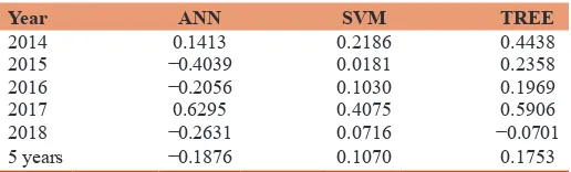
5.3.2. Beta and Treynor ratio
The beta is a measurement of its volatility of returns relative to the entire market. It is used as a measure of risk and is an integral part of the capital asset pricing model. An index with a higher beta has greater risk and also greater expected returns.
The Treynor ratio, also known as the reward-to-volatility ratio, is a performance metric for determining how much excess return was generated for each unit of risk taken on by a stock. Excess return in this sense refers to the return earned above the return that could
have been earned in a risk-free investment. Risk in the Treynor
ratio refers to systematic risk as measured by a stock’s beta. Beta measures the tendency of a stock’s return to change in response to changes in return for the overall market. The higher the Treynor ratio, the better the performance of the stock under analysis.
In Tables 8 and 9, we can see that ANN generates the greater
return, which reaches 59.06%, and yet, its beta is −0.2784 and the resulting Treynor ratio is −0.1876. The reason behind it’s
Table 5: Sharpe ratio index
Year GSPC ANN SVM TREE
2014 0.0629 −0.0444 0.1399 0.1366
2015 −0.0081 0.1136 0.0144 0.1266
2016 0.0556 0.0398 0.0807 0.0691
2017 0.1631 0.0144 0.2100 0.2242
2018 −0.0239 0.0939 0.0489 −0.0368
5 years 0.0301 0.0523 0.0768 0.0795
ANN: Artificial neural network, SVM: Support vector machines
Table 6: Information ratio
Year ANN SVM TREE
2014 −0.0662 0.0895 0.0618
2015 0.0758 0.0353 0.1392
2016 −0.0101 0.0377 0.0117
2017 −0.1054 0.0459 0.0527
2018 0.0715 0.0913 −0.0131
5 years 0.0138 0.0619 0.0471
ANN: Artificial neural network, SVM: Support vector machines
Table 7: Tracking error
Year ANN SVM TREE
2014 1.1553 0.6039 0.8358
2015 1.5608 0.6267 0.9400
2016 1.2652 0.5418 0.9335
2017 0.5915 0.4127 0.4658
2018 1.7589 0.8551 1.0462
5 years 1.3307 0.6253 0.8693
beta’s negative value is that machine learning models’ primary function is to predict stock price movement and buy stocks when
prices rise and short stocks when prices fall. It aims to benefit
both from rising and falling, and thus, its nature resembles active management funds rather than tracking the index. In particular, when markets are most down and corrected predicted by ANN, the returns of ANN strategy will inverse with market returns and generate negative covariance between ANN and market index. In addition to ANN whose beta turns out to be negative, the betas of SVM and random forest fall between zero and one, manifesting that although they are less volatile than the market, their investment performances prove to be more outstanding than that of a benchmark index.
5.3.3. Modigliani ratio
The Modigliani risk ratio, often called M2, measures the return provided by an investment in the context of the risk involved. It was developed by Franco Modigliani and Leah Modigliani in the year 1997.
Modigliani and Modigliani (1997) believed that an ordinary investor would find it easier to understand the Modigliani measure
compared to Sharpe ratio. The reason behind this was that their measure is expressed in percentage points. It shows how well the investor is rewarded for taking a certain amount of risk, relative to the benchmark and the risk free rate.
In general, the riskier an investment is, the less inclined investors will be to put their money into it. So riskier investments have to
offer a higher potential return - that is, deliver a greater profit if the
investment succeeds. In simple words, it measures the returns of an investment index or stock for the amount of risk taken relative to some benchmark index.
In terms of Sharpe ratio, Treynor ratio, Information ratio and Modigliani ratio, the three prediction models all excel
benchmark index. Among them, SVM and Random Forest
outperform ANN.
In brief, conclusions can be elicited from results above that,
firstly, the three machine learning models all exhibit better
investment performance than the S&P 500 index in terms of higher excess returns or less beta volatility. Among them, In
terms of average daily return, SVM and Random Forest generate 2 times higher returns than GSPC (benchmark); with ANN of
1.5 times. For risk-adjusted performance measures, such as the Shape ratio, Jensen’s alpha, information ratio, and Modigliani ratio, machine learning models surpass the benchmark index.
Moreover, among the three machine learning models, Random
Forest generates the best performance, followed by SVM, and ANN coming in last.
6. CONCLUSIONS AND REMARKS
The task-focused in this paper is an analysis of the investment performance of machine learning models. The investment performance of three models namely ANN, SVM, and random
forest are compared based on 5 years (2014-2018) of historical data of the S&P 500 (GSPC) Index.
Experiments show that our proposed machine learning models
generate significantly higher mean returns. In terms of average
daily return, SVM and random forest generate 2 times higher
returns than GSPC (benchmark); with ANN of 1.5 times. Among
the machine learning models, the results indicate that the order of investment performance excellence can be put down as follows: SVM, random forest, and ANN.
For the entire sample period, the cumulative returns of ANN,
SVM, and Random Forest are respectively of 59.06%, 84.55%, and 87.36%. Specifically, in 2015 with a market return of −1.03%, ANN, SVM, and Random Forest are respectively of 28.81%, 4.54%, and 31.96%. Likewise, in 2018 with a market return of −5.69%, ANN and SVM are respectively of 25.87% and 13.90%. Overall, our empirical results suggest machine learning
is promising for higher cumulative returns in the S&P 500 index applications.
Jensen’s alphas of all three machine learning models produce positive values, indicating that their investment performances
surpass that of the benchmark index. Therefore, the sequence of
investment performance excellence can be put down as follows:
Random Forest, SVM, and ANN.
The foremost object of machine learning models is to predict stock price movement and buy stocks when prices rise and short stocks
when prices fall, hoping to obtain profits both from rising and
falling. Therefore, it bears a resemblance to active management funds rather than tracking the index, which accounts for their beta’s negative values and lucrative performance. With regard to the Sharpe ratio, Treynor ratio, Information ratio, and Modigliani ratio, the three prediction models all excel benchmark index.
To sum up, machine learning models exceed benchmark index in investment performance. Among the machine learning models,
Random Forest generates the best performance, followed by
SVM and ANN.
Table 8: Index of risk-adjusted return based on volatility
Indicators ANN SVM TREE GSPC
5 Y return 59.06 84.55 87.36 35.85
Sharpe ratio 0.0523 0.0768 0.0795 0.0301
Jensen’s alpha 0.0549 0.0468 0.0566
Beta −0.2784 0.7153 0.4520
Treynor ratio −0.1876 0.1070 0.1753
Information ratio 0.0138 0.0619 0.0471
Modigliani ratio (M2) 0.0469 0.0670 0.0692 0.0285
ANN: Artificial neural network, SVM: Support vector machines
Table 9: Treynor ratio
Year ANN SVM TREE
2014 0.1413 0.2186 0.4438
2015 −0.4039 0.0181 0.2358
2016 −0.2056 0.1030 0.1969
2017 0.6295 0.4075 0.5906
2018 −0.2631 0.0716 −0.0701
5 years −0.1876 0.1070 0.1753
REFERENCES
Basak, S., Kar, S., Saha, S., Khaidem, L., Dey, S.R. (2018), Predicting the direction of stock market prices using tree-based classifiers. The
North American Journal of Economics and Finance, 47, 552-567.
Bhatia, M., Madaan, A. (2018), Stock portfolio performance by weighted
stock selection. Expert Systems with Applications, 113, 161-185.
Burges, C.J. (1998), A tutorial on support vector machines for pattern recognition. Data Mining Knowledge Discovery, 2(2), 121-167.
Chatzis, S.P., Siakoulis, V., Petropoulos, A., Stavroulakis, E.,
Vlachogiannakis, N. (2018), Forecasting stock market crisis events using deep and statistical machine learning techniques. Expert
Systems with Applications, 112, 353-371.
Chen, A.S., Leung, M.T., Daouk, H. (2003), Application of neural networks to an emerging financial market: Forecasting and trading the Taiwan stock index. Computers and Operations Research, 30(6),
901-923.
Ciner, C. (2019), Do industry returns predict the stock market? A reprise using the random forest. The Quarterly Review of Economics and
Finance, 72, 152-158.
Cortes, C., Vapnik, V. (1995), Support-vector networks. Machine Learning, 20(3), 273-297.
Du, Y. (2018), Application and Analysis of Forecasting Stock Price Index Based on Combination of ARIMA Model and BP Neural
Network. Paper Presented at the 2018 Chinese Control And Decision Conference. Shenyang, China: IEEE.
Grinblatt, M., Titman, S. (1987), The relation between mean-variance efficiency and arbitrage pricing. Journal of Business, 60, 97-112. Grinblatt, M., Titman, S. (1989), Portfolio performance evaluation: Old
issues and new insights. The Review of Financial Studies, 2(3),
393-421.
Grinblatt, M., Titman, S. (1992), The persistence of mutual fund performance. The Journal of Finance, 47(5), 1977-1984.
Gupta, R., Pierdzioch, C., Vivian, A.J., Wohar, M.E. (2018), The predictive value of inequality measures for stock returns: An analysis of long-span UK data using quantile random forests. Finance Research
Letters, 13, 315-322.
Hassan, M.R., Nath, B., Kirley, M. (2007), A fusion model of HMM,
ANN and GA for stock market forecasting. Expert Systems with
Applications, 33(1), 171-180.
Henrique, B.M., Sobreiro, V.A., Kimura, H. (2019), Literature review: Machine learning techniques applied to financial market prediction.
Expert Systems with Applications, 124, 226-251.
Hiransha, M., Gopalakrishnan, E.A., Menon, V.K., Soman, K.P. (2018),
NSE stock market prediction using deep-learning models. Procedia Computer Science, 132, 1351-1362.
Huang, C.S., Liu, Y.S. (2019), Machine learning on stock price movement
forecast: The sample of the Taiwan stock exchange. International
Journal of Economics and Financial Issues, 9(2), 189-201. Jensen, M.C. (1968), The performance of mutual funds in the period
1945-1964. The Journal of Finance, 23(2), 389-416.
Jensen, M.C. (1972), Optimal utilization of market forecasts and the evaluation of investment performance. In: Szego, G.P., Shell, K.,
editors. Mathematical Methods in Finance. Amsterdam: North-Holland Publishing Company.
Kara, Y., Boyacioglu, M.A., Baykan, Ö.K. (2011), Predicting direction
of stock price index movement using artificial neural networks and
support vector machines: The sample of the Istanbul stock exchange.
Expert Systems with Applications, 38(5), 5311-5319.
Kazem, A., Sharifi, E., Hussain, F.K., Saberi, M., Hussain, O.K. (2013), Support vector regression with chaos-based firefly algorithm for stock market price forecasting. Applied Soft Computing, 13(2), 947-958. Khan, W., Ghazanfar, M., Asam, M., Iqbal, A., Ahmad, S., Khan, J.A.
(2016), Predicting trend in stock market exchange using machine learning classifiers. Science International, 28(2), 1-11.
Kim, H.J., Shin, K.S. (2007), A hybrid approach based on neural networks
and genetic algorithms for detecting temporal patterns in stock
markets. Applied Soft Computing, 7(2), 569-576.
Leung, M.T., Daouk, H., Chen, A.S. (2000), Forecasting stock indices:
A comparison of classification and level estimation models.
International Journal of Forecasting, 16(2), 173-190.
Li, X., Xie, H., Chen, L., Wang, J., Deng, X. (2014), News impact on stock price return via sentiment analysis. Knowledge-Based Systems,
69, 14-23.
Li, X., Xie, H., Song, Y., Zhu, S., Li, Q., Wang, F.L. (2015), Does summarization help stock prediction? A news impact analysis. IEEE Intelligent Systems, 30(3), 26-34.
Long, W., Lu, Z., Cui, L. (2019), Deep learning-based feature engineering for stock price movement prediction. Knowledge-Based Systems,
164, 163-173.
Malkiel, B.G., Fama, E.F. (1970), Efficient capital markets: A review of theory and empirical work. The Journal of Finance, 25(2), 383-417. Modigliani, F., Modigliani, L. (1997), Risk-adjusted performance. Journal
of Portfolio Management, 23(2), 45.
Olson, D., Mossman, C. (2003), Neural network forecasts of Canadian
stock returns using accounting ratios. International Journal of
Forecasting, 19(3), 453-465.
Patel, J., Shah, S., Thakkar, P., Kotecha, K. (2015), Predicting stock
and stock price index movement using trend deterministic data
preparation and machine learning techniques. Expert Systems with Applications, 42(1), 259-268.
Qiu, M., Song, Y., Akagi, F. (2016), Application of artificial neural
network for the prediction of stock market returns: The case of the Japanese stock market. Chaos, Solitons and Fractals, 85, 1-7.
Treynor, J.L., Black, F. (1973), How to use security analysis to improve portfolio selection. The Journal of Business, 46(1), 66-86.
Wang, J., Hou, R., Wang, C., Shen, L. (2016), Improved v-support
vector regression model based on variable selection and brain storm optimization for stock price forecasting. Applied Soft Computing, 49, 164-178.
Xi, L., Muzhou, H., Lee, M.H., Li, J., Wei, D., Hai, H., Wu, Y. (2014), A
new constructive neural network method for noise processing and its application on stock market prediction. Applied Soft Computing, 15, 57-66.
Xu, X., Zhou, C., Wang, Z. (2009), Credit scoring algorithm based on
link analysis ranking with support vector machine. Expert Systems with Applications, 36, 2625-2632.
Yang, F., Chen, Z., Li, J., Tang, L. (2019), A novel hybrid stock selection
method with stock prediction. Applied Soft Computing, 80, 820-831.
Zhang, K., Zhong, G., Dong, J., Wang, S., Wang, Y. (2019), Stock