Iranian Journal of Economic Studies
Journal homepage: ijes.shirazu.ac.ir
Sentiment Shock and Stock Price Bubbles in a Dynamic Stochastic General Equilibrium Model Framework: The Case of Iran Ehsan Asadi, Hashem Zare, Mehrzad Ebrahimi, Khosrow Piraiee Department of Economics, Shiraz Branch, Islamic Azad University, Shiraz, Iran.
Article History Abstract
Received date: 10 August 2018 Revised date: 11 October 2018 Accepted date: 22 October 2018 Available online: 11 November 2018
In this study, a model of Bayesian Dynamic Stochastic General Equilibrium (DSGE) from Real Business Cycles (RBC) approach with the aim of identifying the factors shaping price bubbles of Tehran Stock Exchange (TSE) was specified. The above-mentioned model was conducted in two scenarios. In the first scenario, the baseline model with sentiment shock was examined. In this model, stock price bubbles appear endogenously in a positive feedback mechanism that is supported by people optimism. In the second scenario, only sentiment shock is absent from the model. According to the results obtained from the estimation of marginal likelihood model based on Laplace approximation, the baseline model is more in accord with Iran’s economic structure and real data. Consequently, the sentiment shock had a dominant role in creating stock price fluctuations and macroeconomic variables. Based on the results of variance decomposition model, sentiment shock was also recognized as the most important source of fluctuations in bubbles and subsequent fluctuations in stock prices. This shock reflected households’ beliefs about the approximate size of previous bubbles over the recent ones and was passed to the macroeconomic by credit constraints. In this way, this shock also described a major part of the fluctuation of consumption and output. Sentiment shock explained about 86% of stock price fluctuations, 47% of consumption fluctuations, and 39% of output fluctuations.
JEL Classification: E44
E27 E32 E22 G41
Keywords:
The Stock Price Bubble DSGE Modeling Sentiment Shock Real Business Cycles Iran
1. Introduction
One of the fundamental criteria for decision making on a stock exchange is the stock price. If the price index accurately shows the information about the upcoming trends of basic variables; then, we can use it as a leading variable to predict fluctuations in economic activities (Musai et al., 2010). Therefore, since asset prices are effective on the actual allocation of an economy, it is very important to understand the circumstances under which assets prices deviate from their fundamental values (Tirole, 1982). In other words, the price of assets, in addition to fundamental value, can have a bubble component (even if the
component value is zero). The existence of a bubble in asset prices can reduce the efficiency of allocating financial resources to economic production processes. The price bubbles have a one-sided concept of a sharp increase in the stock price in which a huge and short-term price collapse occurs after a continuous increase in the stock price.
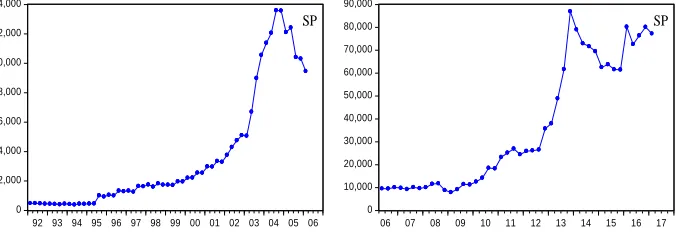
Historical evidence suggests that financial markets are volatile around the world. The stock price index of TSE is known internationally as TEPIX. The study of this index behavior, since the beginning of the stock market reoperation from 1990 to 2017, shows that in many cases the TEPIX has been associated with bubbles. However, in 2005 and 2014, the increasing intensity of the stock price was very large, and it declined at a high rate afterward. The quarterly data of this index between 1992 and 2006 and from 2006 to 2017 is shown in Figure 1. TEPIX peaked suddenly from 2003 to 2005, where it grew by 186% in two years. This index reached from 4756-unit price channel in the second quarter of 2003 to 13596-unit price channel in the second quarter of 2005. After that, during the four seasons ahead, it lost about 30% of its value and returned to the 10411-unit price channel. The above mentioned period can be called the first bubble period. The second major bubble in TSE dates back to 2013 and 2014, where stock prices rose unprecedentedly following the optimism created regarding the nuclear negotiations. TEPIX reached from 38040 in the last season of 2013 to 86957 in the third season of 2014. In just three seasons, it grew by 128%. After this unprecedented growth, the price index lost about 14000 units of its value in less than two seasons and reached about 72969 units.
0 10,000 20,000 30,000 40,000 50,000 60,000 70,000 80,000 90,000
06 07 08 09 10 11 12 13 14 15 16 17
SP
0 2,000 4,000 6,000 8,000 10,000 12,000 14,000
92 93 94 95 96 97 98 99 00 01 02 03 04 05 06
SP
Figure 1. TEPIX graphs for two periods including 1992-2006 and 2006-2017
On the other hand, there is a lot of evidence that accepts the existence of bubbles in asset markets and particularly in stocks. For example, Asadi et al. (2006), Vaez and Torki (2008), Samadi et al. (2010), Abbasian et al. (2010),
Saleh Abadi and Dalirian (2010), and Fallah Shams and Zare (2013) accepted the hypothesis of the existence of bubbles in TSE. Also, the studies done by
in foreign stock exchanges. It is noteworthy that in most studies (especially studies done within Iran) only the existence or absence of stock price bubbles has been addressed and the factors and shocks posing a price bubbles have been neglected.
According to Shiller (1981), stock prices are more volatile than consistent with the asset market efficiency. Thus, studies on behavioral science in the field of financial economics have been expanded rapidly. The emergence of behavioral and psychological dimensions in financial and investment issues and their role in decision making examine the various factors and structures that shape the behavior of investors. Some changes in investor demand for assets are entirely rational and based on information that affects the future growth rates of dividends per share and risk aversion. Nonetheless, Kahenman and Tversky (1979) believed that all changes in demand were not rational, and some were in response to the changes in the expectations or feelings which were not fully supported by the information available. This suggests that investment decisions are not only affected by economic signals and rationality but also by items such as the horizon of investment, the degree of risk tolerance, self-confidence, the belief or assurance that the investor has in mind in the selection and the process of investing in the market. Factors like these have a significant impact on the behavior of investors and their types of decisions. This aspect of financial and investment decision-making was formed to understand and anticipate the interference and influence of psychological decisions in the financial market.
Lee (1993) believed that information cascades were the cause of the price deviation from the fundamental component and the evolution of bubbles. He believed that people, due to their differences in their mental frameworks, would have different perceptions of the same amount of information that provided a source of price deviations. Beltratti and Morana (2006) introduced fad as a factor in creating price bubbles. In their opinion, a fad said to be a deviation from the basic price of the current price, the size of which approximated zero during the time under investigation (Samadi et al., 2010). Beaudry and Portier (2006) described the role of expectations of future technology changes or the “news” shock as a major element responsible for causing fluctuations in macroeconomic variables and stock prices. Samadi et al. (2010) showed that, in the short run, price bubbles in the TSE were justified by imitation behaviors, investors' compliance with fad, and psychological factors. In the long run, the stock price bubbles were linked to the fluctuations beyond the framework of other asset markets.
the factors affecting the stock market price index into two categories: microeconomic and macroeconomic factors. In their opinion, factors such as dividends per share (DPS) and price-earnings ratio (P/E), which are determined in relation to the firm's performance, are micro factors and political and economic factors beyond the control of the firm's management and affecting the entire stock market are macro factors. In this regard, Payandeh Najafabadi et al. (2012) show that the index of TSE is related to the price of oil and gold. According to them, a collapse in TSE index follows a drop in oil price.
Some researchers believe that sentiments, beliefs, and mental status affect decision-making and judgment and, as a result, they cause changes in the investors' behavior. The psychological status of an investor can affect his/her decisions about choosing priorities, risks assessment, reasoning views, and, ultimately, it can affect investment decisions. Therefore, economic decisions will vary based on the different mental statuses of the investors. Hui (2010)
showed that the price of capital assets was directly related to the sentiment and psychological status of the investors. In this regard, higher asset prices relate to a better investor's mental status. In his opinion, integrating the investor's mental status with asset pricing models could help us to interpret the existing evidence of growing abnormalities related to the investors’ behavior. Miao et al. (2015)
argued that, unlike many demand-side shocks such as the news and risk shocks, the sentiment shock was the most important factor in the evolution of price bubbles, and it could create co-movements between stock prices and macroeconomic variables including consumption, investment, working hours, and output. Ikeda (2013) and Bashiri et al. (2016) also identified the sentiment shock as the most important source of stock price bubbles.
Most of the above studies are based on simple regression models or Vector AutoRegressive (VAR) approach and have an unstructured nature and, in some cases, they can be criticized as follows:
First, these models contain only multi-variables and tend to be general. In other words, the effect of one or a very limited number of variables on the dependent variable is examined, and many important variables and parameters are eliminated from the model. Second, they are non-structural in nature and, especially, have to face Lucas’s (1976) criticism in the estimation of the models with constant coefficients (Paetz and Gupta, 2016). Third, both components of bubbles and fundamentals are not visible, and the early literature cannot distinguish between fundamental values and bubbles (Gurkaynak, 2008). Finally, a VAR model or single equation cannot create a time series of the bubble value (Miao et al., 2015). So, it is very difficult to determine if the specifications of bubbles are in accord with the real life.
supply shock and the credit shock are the mentioned shocks in this study. The price bubbles and all of the mentioned shocks are derived from a DSGE model in RBC modeling approach. In this model, stock price bubbles appear endogenously in a positive feedback mechanism that is supported by people optimism. DSGE models respond to Lucas criticism to a large extent. Also, these models are based on rationality and the strong basics of microeconomics. In other words, in this model, the economic system is the outcome of the relationship between agents whose goals and constraints are modeled and interpreted using tools derived from the microeconomic theories (Manzoor and Taghipour, 2016). In addition, the econometric method based on the full information has several advantages over the early literature that uses a regression equation or a VAR model to identify bubbles. In this study, the bubble is considered as a hidden variable in DSGE approach, and the state space in this model permits the Bayesian estimation of hidden variables is linked to information of the real data. So, in the present study, it is possible to simulate a time series of bubbles. Finally, since DSGE is a structural model, various analysis can be made for examining the role of structural shocks in generating bubbles, stock price fluctuations and macroeconomic quantities. In this way, the designed model is challenged in the various conditions as follows: In the first stage, we examine the relative importance of shocks in causing fluctuations in model variables. For this purpose, the role of structural shocks in creating variations in the stock price, output, investment, consumption, and working hours is measured by variance decomposition. The mentioned operation will be done in two scenarios. In the first scenario, each of the seven mentioned structural shocks is present and the baseline model is examined and in the second scenario, there is no sentiment shock in the model. Finally, the impulse response functions (IRF) of model quantities in reaction to shocks will be presented.
The rest of the paper is organized as follows. In section 2, the mechanism of transferring price bubbles to real economy is described. In section 3, a DSGE model constructed. Section 4, deals with research data and initialization. In section 5, the results of the research are analyzed based on the variance decomposition and IRF, and they are summarized in the final section.
2. Stock Price Bubbles and Macroeconomic Variables
instability in economic indexes. According to empirical evidences, there is also a direct link between the financial sector and real economy. In the economic literature, especially in financial economics, the capital market has had an indispensable part in the economic growth of countries through facilitating firms’ financing, allocation of resources, improving the liquidity of assets, and increasing transparency in the economy. Seven and Yetkiner (2016) and Hou and Cheng (2017) have emphasized the positive effect of the stock market on the economic growth. Many economists interpret the decline in the stock price as an economic recession and its rise a sign of economic prosperity.
The fluctuations in the total stock price affect the real activities of the economy through two channels of wealth effect and the change in the investment level. The wealth effect affects the economy through the household and demand-side while the investment channel does so through the firm and supply-side. The wealth effect is justified through Modigliani's (1986) Life Cycle Theory. According to this theory, life-cycle financial resources for consumption come from three sources of human capital, real capital, and financial wealth. Since one of the important components of financial wealth is stock, when the stock prices increase following the formation of bubbles, financial wealth and, consequently, household consumption would increase. This relationship can also occur inversely, when the wealth of households and consumption will decrease in the face of a burst in the price bubbles. For example, findings from a study by Boone et al. (1998) showed that 10% decline in stock prices caused a reduction of at least 45% in the consumption of the US, the UK, and Canada after a year. There are also two views, which are known as the market valuation approach (also known as Tobin's Q) and investment cost approach, on how the fluctuation of stock price affect the firm's investment. Both approaches assume that managers are seeking to maximize their firms’ value when deciding about the investment. According to the market valuation approach, there is a direct relationship between the stock price and investment, and based on the investment cost approach, the stock price indirectly affects investment through a change in the cost of financing to purchase new capital goods. In the capital market approach with the stock price bubbles, the second perspective is considered. When the growth of price bubbles in the firm’s stock increases the firm value, it consequently raises its collateral value to get credit for making the investment. Goyal and Yamada (2004), using firm-level data during the price bubble period, showed that investment significantly responded to stock price bubbles in Japan in the late 1980s. Chaney et al. (2012) also provided similar evidence for the US economy over the period 1993-2007.
The RBC model, in this research, is adjusted based on three common principles: Investment adjustment costs, habit formation, and variable capacity utilization. In addition to these three principles, according to Kiyotaki and Moore (1997), there is a range of firms with random investment opportunities that face endogenous credit constraints. Considering credit constraints in the model is a key assumption. Based on this key idea, firms (borrowers) have limited commitments and may not be forced to repay debt. In this research, the following mechanism is used to force firms to repay debt: In this mechanism, a firm has to commit its assets as guarantees or collateral.
If the firm cannot repay its loan, it will lose its guaranteed asset and the ownership of the firm will be given to the lender. Therefore, the value of collateral for a lender equals to the value of a firm's market with collateral assets. They negotiate debt again; therefore, the debt is constrained to the value of collateral. The result of the negotiation on credit constraint is called collateral constraint. It is assumed that the value of the collateral equals to the going-concern value of the economic unit of a firm re-organized with these assets because the desired value is priced in stock market, and it might include a bubble value. If both the lender and the firm (borrower) of credit constraint are optimistic that the value of the collateral is high1, the firm can borrow more, and lender is willing to lend more. As a result, the firm can finance more investments and build more assets for future production and in fact, make their assets more precious. This mechanism makes the beliefs of lenders and firms (borrowers) act as self-fulfilling and let the bubbles be in the equilibrium. In this study, this equilibrium is referred to as bubbly equilibrium. The existence of a bubble in this positive feedback mechanism will contribute to reducing credit constraints because the bubble prevents the firm from not fulfilling its commitments. Consequently, the firm is able to borrow more to increase investment. Raising investment causes higher firm value, and thus initial optimistic beliefs are justified.
There is also another mechanism for debt repayment, in which case the firm will pay a fine in the event of non-payment of the debt. There is no collateral for the repayment of the loan. If the firm fails, the firm will be permanently removed from the financial market. In a flawless equilibrium, the value of the firm's continuation should be at least as big as the firm's external value in the case of defectiveness that equals the value of the firm’s economic independence when it uses only internal funds to finance the investment. So, the bubble cannot be created after the firm’s failure. The result of these credit constraints is called self-enforcing constraint. Martin and Ventura (2012) have investigated this model of credit constraint.
3. Model
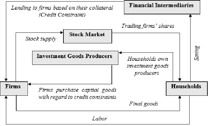
This paper aims to specify a DSGE model for Iran's economy and to simulate macroeconomic variables and stock price bubbles. For this purpose, Bayesian econometric methods and quarterly data are used during the period from 1992:1 to 2017:1 in RBC modeling approach. Adopted by Miao et al. (2012), an economy with an infinite-horizon is considered productive that includes households, firms, capital goods producers, and financial intermediaries. The conceptual model of this study is presented in Figure 2. In this model, households provide firms’ labor, deposit their funds in competitive financial intermediation sectors, and make a profit by trading firm shares in the stock market. Firms also provide final goods for consumption or investment for households. The producers of investment goods produce them on condition of costs adjustment. Firms buy intermediate goods from investment goods producers with regard to credit constraints. The financial capital of firms is determined using internal funds and external borrowing. It is assumed that the firms’ external financing through issuing equity is so expensive that hinders the firm from publishing new ones, and also financial intermediaries utilize households’ deposits to lend to firms. In addition, monetary policy is not considered, and the RBC approach will be studied.
Figure 2. Macroeconomic circular model
Source: Authors’ own compilation
3.1 Households
∑ [ ( ) ] (1)
where ( ) denotes the subjective discount factor, and ( ) represent the habit parameter. Also, represent the labor supply shock. It is assumed that follows the stochastic process as shown below1:
( ) ̅ (2)
Households provide labor for the firm, trade firm shares in a stock market, and owns the investment goods producers. Therefore, the budget constraint is Equation (3):
( ) (3)
where is the aggregate dividends, denotes the aggregate stock price of all the final good producers, is shareholdings, and represents the profits made from the production of capital goods. In equilibrium equals one. The first-order condition of a household is equal to:
(4)
where represent the marginal utility of consumption (MUC) and is obtained from the following Equation:
(5)
3.2 Firms
A representative firm like is chosen from a continuum of identical firms that produces its products by combining its capital and labor based on Cobb-Douglas production function:
( ) ( ) (6)
In Equation (6), 𝛼 ( ) refers to capital elasticity, is the rate of capacity utilization, and represents technology shock. According to this function, might also be referred to as the TFP shock. For a new firm, is considered equal to .
It is assumed that consists of a permanent component and a transitory component , where .The permanent component follows the stochastic process presented as:
( ) ̅ (7)
and the temporary component of this shock follows the stochastic process below:
(8)
In households’ opinions any share of the firm might have a bubble. They also think that this bubble can burst with a certain probability. According to
1 In this paper could be each of the shocks. It is assumed that follows the stochastic process as:
rational expectations, a bubble cannot be re-formed in the same firm. That is when the bubble bursts, then the firm does not contain any bubbles.
To put it crudely, following the Carlstrom and Fuerst (1997), Bernanke et al. (1999) and Gertler and Kiyotaki (2010), the entry and exit of firms are assumed exogenous. A firm may die in any period with an exogenous probability of and its value may reach zero, and a new firm appears in the economy at no cost. Therefore, the overall size of the current firm in each period is fixed. A new firm that arrives at the date with the initial capital starts the
job and acts as a current firm in the same way. The new firm can also take a new bubble to the economy. It is assumed that the amount of depreciation between period t and is ( ). For simplicity, the Steady-State (SS) capacity utilization rate is equal and fixed to 1. In this case the capital stock will be as follows:
( ) (9)
where represents the investment and measures the investment efficiency. It is assumed that of the firm is IID and generates a heterogeneity in the firms. In the following, it is assumed that the decision to use capacity is taken before seeing investment efficiency shocks . As a result, the use of optimal capacity does not depend on this shock. With regard to the wage rate and the rate of capacity utilization , this firm obtains the optimal labor demand by solving the following problem:
( ) ( ) (10)
Thus, the demand for optimal labor equals:
*( ) + (11)
and the capital rental rate is obtained as follows:
𝛼 *( ) +
(12)
In each period, such as t, the firm j can make some investment at price by buying products from the investment goods producers. This is financed by internal funds and external borrowing . In addition, we suppose that this investment at the firm's level is irreversible. Therefore, the firm's investment
is obtained from Equation (13):
(13)
In what follows, and according to Carlstrom and Fuerst (1997), it is thought that there is no interest on loans. Also, as in Miao and Wang’s (2011), the amount of loans determines the following credit constraint:
( )
where ( ) is the firm's cum-dividends stock market value with asset k at the time of t and shows a collateral shock that shows the friction on the financial market (as reported in studies conducted by Jermann and Quadrini (2012) and
Liu et al. (2011)). It is supposed that follows the stochastic process as:
( ) ̅ (15)
Following Miao and Wang (2011), Equation (14) can be considered as a limitation in the contract between the borrower and the lender, in which the firm has restricted commitments.
With regard to this issue, the firm must pledge its assets to the lender in order to take a loan. When the current firm (firm j) wants to borrow money, the lender can find assets . Contrary to what Kiyotaki and Moore (1997) stated in their research, the lender does not instantly deposit the loan to the borrower account and does not immediately sell its assets in the event of non-repayment. In return, the lender allows the firm to continue its operation in the following period. They will once again negotiate this debt. The firm is presumed to have all the bargaining and transaction power. Therefore, the lender is able to compute the risk value ( )
( ) in this loan demand. The
lender is encouraged to lend the loan if the relation (14) is satisfied. Moreover, if relation (14) is established, its incentive will be compatible with the firm; because the value of its continuity and the repayment of the debt would not be smaller than the continuation of non-repayment of the debt:
( )-
( )-( - )
( ) (16)
3.3 Capital Goods Producers
Followed by Gertler and Kiyotaki (2010), capital goods producer makes new investment goods to use them in the production of final goods on the condition of costs adjustment. They sell new investment goods to final goods producers at the price . We can obtain by maximizing the objective function of a capital goods producer as (17):
∑ { [ (
̅ ) ] }
(17)
where ̅ represents the SS growth rate of aggregate investment, is the adjustment cost parameter, and shows the IST shock following Greenwood et al. (1997). It is assumed that is a combination of a permanent component and a transitory component where . The permanent component follows the stochastic process:
( ) ̅ (18)
and will follows the stochastic process:
In Equations (18) and (19), the parameter ̅ represents the SS of growth rate . The first-order conditions of the optimal level of investment goods will be as follows:
(
-
- ̅) ( -
- ̅) -
-
( - ̅ )
(
) (20)
3.4 Decision Making Problem
The firm's j decision making problem is described by the following dynamic programming:
( )
( ) (21)
Subject to (9), (13) and (14). In this way ( ) takes the following form1:
( ) (22)
where 𝜏 is the age of the firm j, and only depend on the idiosyncratic investment efficiency shocks and aggregate state variables. Equation (22) following Hayashi (1982) and Miao et al. (2012) is new. Since competitive markets are considered with CRS technology, this is very common that the firm value is expressed as a linear function. Nonetheless, considering Equation (14), the firm’s value can include bubbles. Thus, if , we have a bubbly equilibrium and if , a bubble-less equilibrium solution is created.
The ex-dividend stock price of the firm at age τ is considered as:
( )
( ) (23)
According to the above speculated form, we have:
(24)
where:
( )
( )
(25)
It should be noted that and do not rely on idiosyncratic shocks
because they can be combined. Furthermore, the marginal Q does not equal to the average Q due to a bubble presence.
3.5 Sentiment Shock
So far, stock bubbles have been considered deterministically. Following
Blanchard and Watson (1982), equilibrium in DSGE models of this study has been constructed by stochastic bubbles. Accordingly, a sentiment shock is introduced about bubble movements for the model of household beliefs and is passed to the macroeconomic by credit constraints. It is assumed that the households believe that with the probability there is a new firm within the time period t containing a bubble as big as . Therefore, the whole
new bubble is obtained with . It is also assumed that they think that the approximate size of the bubbles is created for two firms at 𝜏 that is shown at
t and with . That is:
𝜏 (26)
where follows the below process exogenously:
( ) ̅ (27)
In the present study, this process is considered as a sentiment shock that shows the beliefs of households about variations in bubbles, and they might alter randomly by the passage of time. This process comes from (26):
(28)
Equation (28) shows that the sizes of the current and previous bubbles are related to each other through the sentiment shock, and a change in this shock alters the approximate sizes of these bubbles.
3.6 Equilibrium
It is assumed that ∫ represents the total capital stock of all firms at the end of the period before the death shock is identified, and indicates the aggregate capital stock after the identification of the death shock if a new investment or depreciation does not occur. So that the capital stock is provided using new entrants. As a result, we will have:
( ) (29)
The aggregate labor and output are also defined as ∫ and ∫ . It is assumed that all firms select the same capacity utilization rate. Therefore, all firms have the same ratio of labor to capital. Given CRS technology of the production function, we have:
( ) ( ) (30)
Consequently, the wage rate is provided by equation (31):
( 𝛼) ⁄ (31)
Furthermore, the rental rate of capital is obtained from Equation (32):
𝛼 ⁄ (32)
Also, represents the total bubble in period t. We can write Equation (33) by adding up the bubble of firms of all ages and using (28):
∑ ( )
( ) ( )
( )
(33)
where follows as:
( ) (34)
This variable is stationary in the neighborhood of the SS because ( ) ̅ .
The bubble and marginal Q are considered as a function of used capital.
( - )
[ ( - ) ( ) ] (36)
Accordingly, based on Equations (28) and (35) we can conclude:
( )
( ) (37)
Equation (37) creates an equilibrium limitation on the size of the current bubble. The replacement of Equation (33) in Equation (37) results:
( )
( ) (38)
Equation (38) also shows an equilibrium limitation on the total value of the bubble in macroeconomic. The two mentioned equations block the creation of any kinds of arbitrage chances in new and previous bubbles. Equations (34) and (38) show the effects of a sentiment shock on the approximate size and followed by the total bubble.
Given the total value of all firms in Equation (24), we consider the aggregate stock price of firms as Equation (39):
(39)
Equation (39) shows that the aggregate stock price includes two values: The fundamental component and the bubble component .
On the other hand, ∫ represents the aggregate investment. Assuming, firstly, that the optimal level of firm j investment is accompanied by bubble and, secondly, that the rate of capacity utilization for each firm is the same and also using the firms adding up property of all ages, we drive the aggregate investment for bubbly firms through a law of large numbers, so that:
[( ) ]∫
( ) (40)
Similarly, the capital stock for these firms will be as follows:
( ) ∫ ( )
∫
( )
∫
( ) (41)
where we need a law of large numbers and the fact that and are independent. And the resource constraints are given as follows:
[ (
̅ ) ] (42)
Finally, a competitive equilibrium including stochastic processes that has sixteen aggregate endogenous variables, {
} and seven stochastic structural shocks is generated.
summarized in equations (43-66)1. All symbols have been presented in the previous sections.
1. Resources constraints
̂ ̃ ̃ ̂ ̃ ̃ ̂ (43)
2. Aggregate Investment
̂
̅ ̃ ⁄ ̃ ̂
̅
̅ ̃ ⁄ ̃( ̂ ̂ ̂ )
̃ ⁄ ̃ ̅ ̃ ⁄ ̃ ̂
̂ ̂
(44)
3. Aggregate Output
̂ 𝛼( ̂ ̂ ) ( 𝛼) ̂ (45)
4. Labor Supply
̂ ̂ ̂ ̂ (46)
5. Capital stock
̂ ( ) ̂ ( ) ̂ ( ( )) ( ̂ ̂ ) (47)
where ( ) and
( ) ̅ .
6. Capacity utilization
̂ ̂ [ ( ) ̅] ̂ ̂ ( ( )
( )) ̂ (48)
7. Marginal Q
̂ ( ̂ ̂ ) ( ̂ ̂ ̂ ) ( ) ( )
̅
( )
( ) ̂
̅ ( )
̅ ( ̂ ̂ )
(49)
8. Effective capital stock
̂ ̅ ( ̂ ̂ ̂ ) (50)
9. Total value of the bubble
̂ ( ̂ ̂ ̂ ) [ ( ) ̅] ̂ ( ) ̅
( ) ̅ ̂
(51)
10. Number of bubbly firms
̂ ( ) ̅ ̂ ( ) ̅ ̂ (52)
11. Investment goods price
̂ [( ) ̅ ̂ ̅ ( ̂ ̂ ) ̅ ̂
̅ ( ̂ ̂ ̂ )]
(53)
1 It should be noted that the DSGE model has been designed in such a way that the relations between
equations can be obtained, irrespective of the rental rate and the wage rate . In this way, these two variables are eliminated from the equilibrium equations, and instead of them, the equations (57) and (58) are added to the log-linearized equations, where ̂ is the growth rate of the investment goods price and ̂ represents the growth rate of consumption goods that are used to eliminate unit root in the
12. Marginal utility for consumption
̂
[ ̂ ( ̂ ̂ )]
[ ( ̂ ̂ ) ̂]
(54)
13. Stock price
̂ ̃ ̃
̃( ̂ ̂) ̃
̃ ̂ (55)
14. Investment efficiency
̂ ̂ ̂ (56)
15. The growth rate of the investment goods price
̂ ̂ ̂ ̂ (57)
16. The growth rate of consumption goods
̂ ( ̂ ̂ ̂ ) ( ̂ ̂ ̂ ) (58)
Due to the fact that Iran's working hours are not available, instead, employment data is used in this research. As the employment variable tends to react more slowly to macroeconomic shocks than aggregate working hours, following Smets and Wouters (2003) and Zagaglia (2009), it is assumed that in each period only a part of firms dismiss their labor forces. In this way, the following equation is exogenously added to the log-linearized equation of this research:
17. Employment heads equation
̂ ̂
( )( )
( ̂ ̂ ) (59)
where ̂ is the fluctuations in working hours and ̂ is the fluctuations in the number of employees. Also, shows a part of firms that dismiss their labor forces.
The processes of log-linearized shocks are also listed Equations (60-66):
1. The permanent TFP shock
̂ ̂ (60)
2. The transitory TFP shock
̂ ̂ (61)
3. The permanent IST shock
̂ ̂ (62)
4. The transitory IST shock
̂ ̂ (63)
5. The labor supply shock
̂ ̂ (64)
6. The credit shock
̂ ̂ (65)
7. The sentiment shock
Finally, the log-linearized model of this research included 24 equations and 24 endogenous variables by adding the employment equation and seven structural shocks.
There may be two types of equilibrium in this model: The bubbly equilibrium where is for all t and the bubble-less equilibrium in which
is also for all t. Households believe that there are no bubbles in old or new firms in a bubble-less equilibrium, meaning ( ). In the present study, with the aim of identifying the factors affecting price bubbles of TSE, the baseline model, meaning the bubbly equilibrium model, will be used. 4. Data and Parameters Initialization
The data used in this research have been collected from the Central Bank of the Islamic Republic of Iran which include the quarterly data of Gross Domestic Production (GDP), private consumption, private investment, stock price, and employment in the period 1992:1-2017:1. All data were seasonally adjusted, logged, and de-trended by Hodrick-Prescott Filter ( )1. To be more in accord with the reality, since the economy under study has two sectors (without the government and foreign sectors), the GDP data was derived from the sum of the private consumption and private investment.
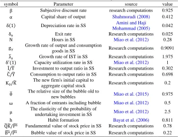
Initialization of model parameters using three calibration methods based on previous studies, research computations and estimation in the Bayesian method are obtained. In this way, the initialization of the parameters of the DSGE model was divided into two categories: The first category of parameters, as presented in Table 1, was derived from two calibration methods based on previous studies and computations of the research. The meaning of initialization based on the computations of the research was the amounts of parameters that were firstly consistent with the literature of the DSGE models, and secondly, the greatest approximation was obtained between the moments of the simulated and real data. It should be noted that among these parameters, there were also the ratio of some variables that were derived from the division of the two variables in the SS.
1
Table 1. Parameters initialization
value source
Parameter symbol
0.925 research computations
Subjective discount rate
0.412 Shahmoradi (2008)
Capital share of output α
0.042 Amini and Haji
Mohammad (2005) Depreciation rate in SS
( )
0.025 Research computations
Exit rate
0.28 Miao et al. (2012)
Hours in SS
0.9091 Research computations
Growth rate of output and consumption goods in SS
1.975 Research computations
Growth rate of IST in SS ̅
1 Miao et al. (2012)
Capacity utilization rate in SS ( )
0.302 Research computations
Investment to output ratio in SS ̃ ̃
0.698 Research computations
Consumption to output ratio in SS ̃ ̃
0.2 Research computations The new firm's initial capital to
aggregate capital stock ̃
0.975 Miao et al. (2015)
The relative size of the bubble old to new bubbles
̅
0.5 Miao et al. (2012)
A fraction of entrants including bubble ω
2.5 Miao et al. (2012)
The elasticity of the probability of undertaking investment in SS μ
0.811 Bayat et al. (2006)
Habit formation
0.78 Research computations
Fundamental value of stock price in SS ̃ ̃ ̃
0.22 Research computations
Bubble value of stock price in SS ̃ ̃
Table2. The result from Bayesian estimation of parameters posterior source Prior distribution Prior (Mean & S.E) parameter symbol 2.4627 Liu et al. (2011)
Gamma (2,2)
Investment cost adjustment parameter
3.2858 Miao et al. (2012)
Gamma (1,1) Capacity utilization parameters ( ) ( ) 0.2820 Miao et al. (2015)
Beta (0.3,0.1)
Average degree of credit constraint ̅ 0.9213 Zagaglia (2009) Beta (0.5,0.15)
A fraction of firms that can adjust their
labor forces 0.6523 Smets and Wouters (2007) Beta (0.5,0.2) Persistence parameter of the permanent TFP
shock 0.4561 Smets and Wouters (2007) Beta (0.5,0.2) Persistence parameter of the transitory TFP
shock 0.4536 Smets and Wouters (2007) Beta (0.5,0.2) Persistence parameter of the permanent IST
shock 0.5571 Smets and Wouters (2007) Beta (0.5,0.2) Persistence parameter of the transitory IST
shock 0.7071 Smets and Wouters (2007) Beta (0.5,0.2) Persistence parameter of the labor supply
shock
0.4990 Liu et al. (2011)
Beta (0.5,0.2)
Persistence parameter of the credit constraint shock
0.5970 Miao et al. (2012)
Beta (0.5,0.2)
Persistence parameter of the sentiment
shock
0.0113 Liu et al. (2011)
INV-Gamma (0.01, INF)
S.D. of the permanent TFP shock
0.0569 Liu et al. (2011)
INV-Gamma (0.01, INF)
S.D. of the transitory TFP shock
0.0066 Liu et al. (2011)
INV-Gamma (0.01, INF)
S.D. of the permanent IST shock
0.0602 Liu et al. (2011)
INV-Gamma (0.01, INF)
S.D. of the transitory IST shock
0.1675 Liu et al. (2011)
INV-Gamma (0.01, INF)
S.D. of the labor supply shock
0.0085 Liu et al. (2011)
INV-Gamma (0.01, INF)
S.D. of the credit constraint shock
0.6000 Miao et al. (2015)
INV-Gamma (0.01, INF)
S.D. of the sentiment shock
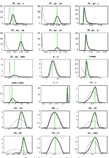
The second category of parameters was estimated using the Bayesian method. The Bayesian approach requires the prior information to be specified for the parameters to be estimated. Usually, in this case, previous information about parameters and its distribution are taken from previous studies and the economic literature. The prior information reflects the researcher’s or the modeler's guess before examining the hidden information in the sample data, and it provides additional information for estimating the parameters. The prior information is explained through the prior probability density function, while the hidden information in the sample observations is described through the likelihood function. The multiplication product of these two distributions, based on the Bayes’ Theorem, results in a new distribution that is called the posterior probability distribution, and later judgments and decisions that are made in the modeling process will be based on this distribution (Shahmoradi and Ebrahimi, 2010). Therefore, the posterior distribution of parameters in this study was calculated using Metropolis-Hastings (MH) Algorithm with 200,000 repetitions using the Dynare software. Posterior distribution of parameters accompanying their prior mean and standard deviations (SD), which have been taken from the previous studies, are reported in Table 2 and Figure a1 (in appendix).
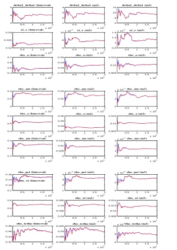
To assess the ability of the model in relation to the estimation of the parameters, the acceptance ratio in the MH algorithm and the convergence diagnostic test of Brooks and Gelman (1998) in Monte Carlo Markov Chain (MCMC) process were used. The acceptance ratio in the MH algorithm in the estimation process is ideally in the range of 25% to 33%. The estimated results showed that this value was in the three-chain algorithm in the ideal range. The result is presented in Table 3:
Table 3. Current acceptance ratio per chain
Metropolis-Hastings algorithm Chain 1 Chain 2 Chain 3
The acceptance ratio 31.9813 32.3613 31.0183
Source: Research findings
Another criterion for evaluating the estimates is the convergence diagnostic test of Brooks and Gelman (1998) in the MCMC process. The univariate and multivariate diagnostic graphs of the MCMC are a major source of reliability assessment of estimates. The Dynare software reports three measures for this test. The “interval measure” is based on a confidence interval of 80% around the parameter mean, “m2 measure” is based on an 80% confidence interval around the variance of the parameter, and “m3 measure” is based on a confidence interval of 80% around the third moments of the parameter. Figure a2 (in appendix) illustrates that the two drawn graphs for the first to third moments of each parameter moved to each other and at the same time to a constant value, which means that the estimates were correct.
moments converged quite well and tended to a constant value at the same time. The result showed the reliability of the overall model estimation.
Figure 3. MCMC multivariate convergence diagnostic test
Source: Research findings
In addition, we report the baseline model’s forecasting regarding SDs relative to output, correlation with output, and the first order autocorrelations in Table 4. Moments were computed using both real data and the simulated data when seven shocks were turned on. Variables were seasonally adjusted, logged, and de-trended by HP Filter.
Table 4. Business Cycles Statistics
DATA Output
(Y)
Consumption (C)
Investment (I)
Stock Price (SP)
Employment (EH) Standard Deviations Relative to Y
Real data 1.000 0.927 1.930 4.069 0.116
Simulated
data 1.000 0.970 1.123 3.671 0.104
Correlation with Y
Real data 1.000 0.846 0.797 0.262 0.176
Simulated
data 1.000 0.992 0.967 0.762 0.457
First Order Autocorrelations
Real data 0.303 0.254 0.560 0.760 0.929
Simulated
data 0.847 0.875 0.780 0.972 0.911
Source: Research findings
The results showed that all series were pro-cyclical with output and the difference between real data and simulated data were small.
0.2 0.4 0.6 0.8 1 1.2 1.4 1.6 1.8 2
x 105
6 8 10
Inte rval
0.2 0.4 0.6 0.8 1 1.2 1.4 1.6 1.8 2
x 105
5 10
15 m2
0.2 0.4 0.6 0.8 1 1.2 1.4 1.6 1.8 2
x 105
0 50 100
5. Results
The results of the variance decomposition of variables in response to the occurrence of any structural shocks were done in two scenarios: In the first scenario, each of the seven introduced structural shocks was present, and the baseline model of the research was examined. In the second scenario, the sentiment shock was absent from the model. The results are given in Tables 5 and 6:
Table 5. Variance decomposition of variables relative to structural shocks (Baseline model)
Shocks Output
(Y)
Consumption (C)
Investment (INV)
Stock Price (SP)
Hours (N) The Permanent TFP
shock 1.10 1.15 0.90 0.09 1.75
The transitory TFP
shock 16.23 18.04 11.60 0.23 28.05
The Permanent IST
shock 0.81 0.66 1.10 0.11 0.44
The transitory IST
shock 16.93 10.12 33.69
*
0.94 7.34
The labor supply shock 25.88 22.44 31.09 12.68 47.61*
The credit constraint
shock 0.0002 0.0001 0.0004 0.001 0.0000
The sentiment shock 39.05* 47.59* 21.62 85.94* 14.82
Source: Research findings
Note: The symbol * denotes the most important structural shock in the variable fluctuation.
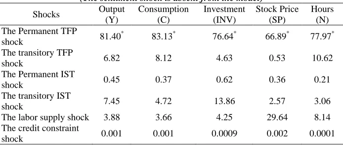
Table 6. Variance decomposition of variables relative to structural shocks (The sentiment shock is absent from the model)
Shocks Output
(Y)
Consumption (C)
Investment (INV)
Stock Price (SP)
Hours (N) The Permanent TFP
shock 81.40
*
83.13* 76.64* 66.89* 77.97*
The transitory TFP
shock 6.82 8.12 4.63 0.53 10.62
The Permanent IST
shock 0.45 0.37 0.62 0.36 0.21
The transitory IST
shock 7.45 4.72 13.86 2.57 3.06
The labor supply shock 3.88 3.66 4.25 29.64 8.14
The credit constraint
shock 0.001 0.001 0.0009 0.002 0.0001
Source: Research findings
Note: The symbol * denotes the most important structural shock in the variable fluctuation.
largest share in the fluctuations in model variables. This result is not unexpected because according to the RBC literature, the technology shock has a decisive and vital part in the fluctuations in macroeconomic variables.
To compare the function of the baseline model with the one without the sentiment shock, marginal likelihoods based on the Laplace approximation was used. According to the results, the log marginal likelihoods for the baseline model and the alternative model equaled 918.323 and 907.048, respectively. These results showed that the baseline model was more compatible with the structure of Iran's economy and the real data. Therefore, it could be concluded that the sentiment shock plays an important role in the evolution of stock price bubbles. Accordingly, the focus should be on the results of the baseline model.
Variance decomposition of the variables in the baseline model showed that the sentiment shock had the largest role in explaining stock market fluctuations. This shock represented about 86% of stock price fluctuations. In addition, the sentiment shock had the largest share in output and consumption fluctuations. About 39% of output fluctuations and more than 47% of consumption fluctuations were justified by this shock. It also had a large share (about 22%) in investment fluctuations; although the largest share in investment fluctuations belonged to the transitory IST shock. Ultimately, the sentiment shock accounts for about 15% of employment fluctuations, while half of the employment fluctuations was limited to the labor supply shock, and more than 28% of the variable fluctuations were justified by the transitory TFP shock.
To better understand the reason behind these results, the log-linearized equation of stock prices presented as:
̂ ̃ ̃
̃(̂ ̂ ) ̃
̃̂ (67)
where the log-linearized equation of the price bubble is shown in the form:
̂ - ̂ [ - ( - )̅] ∑ (̂ - ̂ ) -( - ) ̅
( - ) ̅ ∑ ̂ (68)
In Equation (68), denotes a negative value. Equation (67) shows that the stock price fluctuationŝt
s
are determined by marginal Q fluctuationŝt, capital stock variationŝt , and fluctuations inthe bubble ̂ . According to the economic studies, the capital stock is a low-fluctuating variable, and it cannot explain the stock price fluctuations. The variations of marginal Q are only significant when the investment adjustment cost parameter is high. Based on the research estimation, this is not very large (based on Bayesian estimation, ). Thus, a change in the marginal Q cannot create a big fluctuation in the stock price. On the other hand, Equation (68) shows that bubble variations are mainly determined by the change caused in the expected relative size of the total bubble to the current bubble ̂ , since the changes ̂ and ̂ will be small
specified trough the sentiment shock ̂ . Thus, based on the results of this
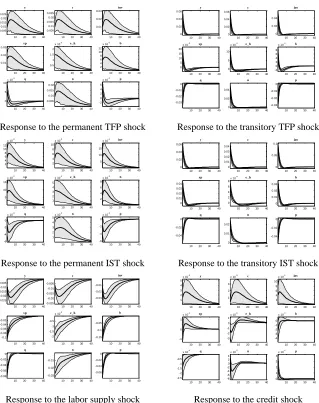
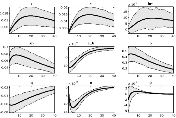
research, the sentiment shock had a significant role in stock price fluctuations1. In order to understand the impacts of these seven structural shocks on the variables, the IRF of these shocks are depicted in Figures 4 and 5. In these figures, the symbols y, c, inv, sp, e_h, b, q, n, and p represent the output, consumption, investment, stock price, employment, bubble, marginal Q, working hours and the capital goods price, respectively. The vertical axis of each graph in Figures 4 and 5 shows the variation percentage of variables from their values in the SS, and the horizontal axis represents the periods (here each period is equivalent to one quarter).
The top-left panel in Figure 4 reflects that a permanent TFP shock cannot be a vital driving force in TSE changes. This shock decreases the marginal Q because it lowers the future MUC because of the wealth effect. Although this shock increases bubble in stock prices, its effect on stock prices is small. As this panel shows, the effect of permanent TFP on stock prices is close to its impact on aggregate macroeconomic variables. It implies that if the permanent TFP shock is the stimulating force, the fluctuations of TSE will be close to the growth of the output. While standard deviation of stock price growth in Iran's real data is much larger than output, consumption, and investment. Similarly, although a positive transitory TFP shock, at the top-right panel in Figure 4, reduces the marginal Q and increases the bubble, as this panel shows, its effect on stock prices is low relative to aggregate macroeconomic variables. Therefore, this shock also cannot describe the relative fluctuations in TSE. Both permanent and transitory TFP shocks increased the working hours in the current study, although these shocks could have led to the loss of hours, because of the existence of consumption habit formation and the investment adjustment cost. As the value of was not large in the present research, the TFP shock increased the working hours.
Based on the results of the IRF, a transitory or permanent IST shock cannot be the main driving force of TSE change since the price of capital goods is counter-cyclical, but the TSE value is pro-cyclical. As shown at the middle panel in Figure 4, in response to an IST shock, both the price of capital goods and marginal Q declined for the reason that this shock increased the capital stock. Therefore, the fundamental component of the stock price
decreases since the capital variable is slowly adjusted, and when the marginal Q decreases, the additional gain of investment also drops. This suggests that the shadow value of the expansion of the credit constraint will decrease too. Since the bubble size is determined through this shadow value, the bubble value also decreases as shown in (68).
The transitory IST shock creates a substitution effect and decreases consumption. Therefore, MUC increases and reduces the size of the bubble
1
value. On the other hand, a growth in MUC and the capital decreases the marginal Q that results in a rise in the bubble value. The net effect of a positive transitory IST shock equals the rise in stock prices. However, the size of stock price variations is less than the investment and output after a transitory IST shock. In contrast, a positive permanent IST shock has a huge impact on the wealth of households and increases consumption.
Response to the permanent TFP shock Response to the transitory TFP shock
Response to the permanent IST shock Response to the transitory IST shock
Response to the labor supply shock Response to the credit shock
Figure 4. Impulse response graphs of variables in response to structural shocks
Source: Research findings
10 20 30 40 0.005 0.01 0.015 0.02 0.025 y
10 20 30 40 0.005 0.01 0.015 0.02 0.025 c
10 20 30 40 0.01
0.02 0.03
inv
10 20 30 40 0.01
0.02 0.03
sp
10 20 30 40 0.5
1 1.5 2
x 10-3 e _h
10 20 30 40 2 4 6 8 10 12
x 10-3 b
10 20 30 40 0
5 10
x 10-3 q
10 20 30 40 0.005
0.01 0.015 0.02
n
10 20 30 40 -2
0 2 4 6
x 10-3 p
10 20 30 40 0
0.02 0.04 0.06
y
10 20 30 40 0
0.02 0.04 0.06
c
10 20 30 40 0
0.02 0.04
inv
10 20 30 40 0
5 10 15 20
x 10-3 sp
10 20 30 40 0
5 10
x 10-4 e _h
10 20 30 40 -2 0 2 4 6 8
x 10-3 b
10 20 30 40 -0.03
-0.02 -0.01 0
q
10 20 30 40 0
0.02 0.04
n
10 20 30 40 -0.03
-0.02 -0.01 0
p
10 20 30 40 2 4 6 8 10 12
x 10-3 y
10 20 30 40 2
4 6 8 10
x 10-3 c
10 20 30 40 5
10 15
x 10-3 inv
10 20 30 40 5
10 15
x 10-3 sp
10 20 30 40 1
2 3 4 5
x 10-4 e_h
10 20 30 40 2
4 6 8
x 10-3 b
10 20 30 40 -6
-4 -2 0
x 10-3 q
10 20 30 40 1
2 3 4 5x 10
-3 n
10 20 30 40 -6
-4 -2 0
x 10-3 p
10 20 30 40 0
0.02 0.04 0.06
y
10 20 30 40 0 0.01 0.02 0.03 0.04 c
10 20 30 40 0
0.05 0.1
inv
10 20 30 40 0 0.01 0.02 0.03 0.04 sp
10 20 30 40 0
2 4 6 8x 10
-4 e_h
10 20 30 40 0
0.01 0.02 0.03
b
10 20 30 40 -0.04
-0.02 0
q
10 20 30 40 0
0.01 0.02
n
10 20 30 40 -0.04
-0.02 0
p
10 20 30 40 -0.025 -0.02 -0.015 -0.01 -0.005 y
10 20 30 40 -0.025 -0.02 -0.015 -0.01 -0.005 c
10 20 30 40 -0.03
-0.02 -0.01
inv
10 20 30 40 -0.1 -0.08 -0.06 -0.04 -0.02 sp
10 20 30 40 -2
-1.5 -1 -0.5
x 10-3 e_h
10 20 30 40 -0.15
-0.1 -0.05
b
10 20 30 40 -0.08 -0.06 -0.04 -0.02 0 q
10 20 30 40 -0.03
-0.02 -0.01
n
10 20 30 40 -0.06
-0.04 -0.02 0
p
10 20 30 40 1
2 3 4 5
x 10-5 y
10 20 30 40 1
2 3
x 10-5 c
10 20 30 40 2
4 6 8 10
x 10-5 inv
10 20 30 40 -1
0 1
x 10-4 sp
10 20 30 40 -3
-2 -1 0 1
x 10-6 e_h
10 20 30 40 -4
-3 -2 -1 0
x 10-4 b
10 20 30 40 -2.5
-2 -1.5 -1 -0.5
x 10-4 q
10 20 30 40 -8 -6 -4 -2 0 2 4
x 10-5 n
10 20 30 40 0
1 2 3 4
Figure 5. Impulse response graphs of variables in response to the sentiment shock
Source: Research findings
Accordingly, the marginal utility flow declines and the bubble size increases by Equation (68). This effect can overcome the decreasing effect in marginal Q and increases the bubble reaction to positive permanent IST shock. Eventually, the increase in the bubble components due to this shock will be more than the reduction of fundamental components and will increase stock prices following a permanent IST shock. Based on the results, impulse responses to both transitory and permanent IST shocks represent a pro-cyclical movement of the stock price although these shocks represent a small fraction of stock price fluctuations.
The bottom-left panel in Figure 4 shows that labor supply shock took a noteworthy gap in aggregate macroeconomic variables. This shock was a reduced-form shock capturing the labor wedge. This labor supply shock increased the marginal utility of leisure (MUL), and thus, it declined working hours and consumption. This shock increased MUC so that the marginal Q, the bubble size, and the stock price also reduced. As the labor supply shock directly influences the MUL, it is very essential to describe changes in working hours. Interestingly, the reaction of working hours to employment is faster and more volatile in response to all shocks of this research. In this study, by accepting the fact that the employment was slower and less fluctuating than working hours due to rigidities and the existence of contracts, the relationship between employment and working hours was modeled in such a way that only a part of firms adjusted their labor force in each period. Since the parameter of this
10 20 30 40
0.005 0.01 0.015
y
10 20 30 40
0.005 0.01 0.015 0.02
c
10 20 30 40
0 5 10 15
x 10-3 inv
10 20 30 40
0.04 0.06 0.08 0.1
s p
10 20 30 40
-10 -5 0
x 10-4 e _h
10 20 30 40
0.2 0.3 0.4 0.5
b
10 20 30 40
-0.08 -0.06 -0.04 -0.02
q
10 20 30 40
-15 -10 -5 0
x 10-3 n
10 20 30 40
-6 -4 -2 0 2
equation was smaller than one, it was natural that the fluctuation of working hours be greater than the employment.
Based on economic studies, the role of the credit shock is said to be very important in business cycles. The credit shock propagates through credit constraints because it directly affects the capacity of the firm's borrowing. The bottom-right panel in Figure 4 indicates that when the TSE data is considered, the share of credit shock decreases. It is thought that increasing credit shocks reduce credit constraints; thus, it increases the investment. This demand growth in the investment increases the capital goods price. On the other hand, when capital stock increases, marginal Q decreases and leads to a reduction in the fundamental value. In addition, the credit shock will also be less effective on the bubble component since firms do not have any interest to generate a big bubble before reducing credit constraints. Consequently, the net effect of a growth in the credit shock reduces the stock price and shows that a credit shock is not able to run TSE in the direction of the cycle. In addition, this shock will slightly increase the consumption (much less than the investment). As a result, the credit shock cannot create an equal movement between stock prices and macroeconomic variables including investment, consumption, and output, and its effect on the stock price fluctuations and real economic variables would also be very low.
shock. But when households believe that the future value of a firm’s stock will not be higher than its current value, the above trend will be shaped in the opposite direction, and the stock market, consumption, investment and output will decline altogether. This result suggests that the peak of the TSE will be accompanied by households' sentiment optimism about the growth of bubbles, and on the contrary, the collapse of this market will be associated with the households' sentiment pessimism about the burst of bubbles.
6. Concluding Remarks
In this study, according to Miao et al. (2012), a Bayesian DSGE model from TSE bubbles and RBC approach were specified, estimated, and simulated. Stock price bubbles in this model appear endogenously in a positive feedback mechanism that is supported by people’s optimism. In the model adopted in this research, a sentiment shock was identified that controlled both bubble and stock price variations. This shock reflected households’ beliefs about the approximate size of previous bubbles over the recent ones and was passed to the macroeconomic by credit constraints. This shock generate fluctuation in the collateral value so it is effective in the firm’s decision making about the investment and output.
To better identify the impact of this shock on the creation of price bubbles, followed by stock price fluctuations, the DSGE model used in this research was conducted in two scenarios: In the first scenario, the baseline model of the research was examined by seven structural shocks; in the second scenario, only the sentiment shock was absent from the model. According to the results of the marginal likelihoods model based on Laplace's approximation, the baseline model was more in accord with Iran’s economic structure and real data, which meant that the sentiment shock had played a crucial factor in stock prices fluctuations and Iran's economy.
Based on the results of the variance decomposition of the variables in baseline model, the sentiment shock was also introduced as the most important source of bubble fluctuations, followed by fluctuations in stock prices. This shock also expresses a large part of the consumption and output fluctuations. A sentiment shock explained about 86% of stock price fluctuations, 47% of consumption fluctuations, and 39% of output fluctuations. Although the largest contribution belonged to the transitory IST shock in investment fluctuations, the sentiment shock share (about 22%) in investment fluctuations should not be ignored. Ultimately, the sentiment shock also accounted for about 15% of employment fluctuations, while half of the employment fluctuations was limited to the labor supply shock, and more than 28% of this variable fluctuation was justified by the transitory TFP shock.
the sentiment shock in TSE appeared as wealth effects and the effect of sentiment shock on the consumption was more than its effect on the investment and working hours. According to the results of this study, a sentiment shock had a significant impact in stock price variations and macroeconomic fluctuations.
Theoretical foundations, model structure, and results of research data show that price bubbles emerge from the sentiment and optimism of households by reducing credit constraints. In this case, bubbles will not have a negative effect on the economy, and even increase production, investment, and consumption. However, the negative effect of price bubbles appears when there are problems of intermediating between financial creditors (usually banks) and investors. In other words, investors or firms face credit constraints. This means that investors do not use their loans according to the lenders or policymakers' objectives and use most of these loans to buy assets such as housing and stocks, which have a limited supply. Since the supply of these assets is constant, the prices are above the fundamental value and the bubble is formed with negative effects. Of course, this may also occur the other way round where lenders in the credit market instead of giving loans to investors (firms) purchase firm shares directly with the incentive to earn more profit than the profit from paying credit to loan applicants. In this case, the demand for assets will increase over its limited supply and provides the ground for rising asset prices and bubble formation with negative effects. In the situations where bubbles have negative impacts on the economy, two policies are proposed:
1. Lenders in the credit market do not do anything other than their specialized field, namely, receiving deposits and proving facilities (and of course, activities such as electronic banking and the acquisition of profits through fees that are not included in this discussion). In other words, they do not do business; otherwise, given limited financial resources, they face firms and investors with credit constraints and intensify the negative effects of bubbles. Credit constraints reduce the growth of investment and do not support the initial optimism of households. Therefore, it is suggested to direct financial resources to firms.
2. Firms and investors use facilities only in investment and production. In this way, it is proposed to closely monitor firms’ performance.