Common weights for the evaluation of decision-making units with nonlinear virtual inputs and outputs

167

Available online at http://ijdea.srbiau.ac.ir

Int. J. Data Envelopment Analysis (ISSN 2345-458X)

Vol. 1, No. 3, Year 2013 Article ID IJDEA-00135, 7 pages

Research Article

Common weights for the evaluation of

decision-making units with nonlinear virtual inputs and

outputs

S. Borzoeia_{, M.Zohrehbandian}a

(a) Department of Mathematics, Karaj Branch, Islamic Azad University, Karaj, Iran.

Received 21 August 2013, Accepted 26 September 2013

Abstract

In this paper, by investigating the common weights concept and DEA models with nonlinear virtual inputs/outputs, we introduce a model for evaluating the decision making units with nonlinear virtual

inputs and outputs based on the common weights.

Keywords: Data envelopment analysis, Common weights, Nonlinear virtual inputs/outputs.

1. Introduction

Data envelopment analysis (DEA) obtains the efficiency measurement of decision making units (DMUs) with multiple inputs/outputs based on the ratio of weighted outputs to weighted inputs, where each DMU can take the desirable weights for inputs/outputs to provide the maximum performance. But the evaluation of DMUs based on the selection of different set of weights is unacceptable.

Therefore, some researchers by linking DEA with some other techniques such as multi-objective programming, have developed models to generate a set of common weights for evaluating and ranking the DMUs (see Roll and Golany [9], Doyle [6] , Bylton and Vickres [1], Lee and Reeves [8], Kao and hung [7], Chen et al [2] and Zohrehbandian et al [10]).

In addition, Cook et al [3] and Cooper et al [4] have assumed linear input/output models in DEA as unreal properties and by considering Piecewise linear form for them, they tried to provide a model for evaluating DMUs in more realistic situations. Moreover, Despotis et al [5] have proposed a general formula by considering nonlinear virtual inputs/outputs in DEA models.

Tel:+989122124384

[email protected] borz

Sajad

:

mail addresses

-E

Corresponding author



168 S.Borzoei, et al /IJDEA Vol.1, No. 3 (2013).167- 173

In this paper, a common weight model with nonlinear virtual inputs/outputs will be presented, which is the idea of the combination of common weights models and nonlinear virtual inputs/outputs concept. The rest of the paper is as follows. In section 2, nonlinear virtual inputs/outputs and common weight concepts will be reviewed. Section 3 presents a common weight model with nonlinear virtual inputs/outputs. Section 4 includes numerical example while section 5 is devoted to concluding remarks

2. Preliminaries and notations

2.1 - Model with nonlinear virtual inputs/outputs

Suppose we have n DMUs with m inputs and s outputs. CCR model to assess the performance unit o is as the following form:

Max ∑𝑠_𝑟=1𝑢_𝑟𝑦_𝑟𝑜 s.t. ∑𝑚_𝑖=1𝑣_𝑖𝑥_𝑖𝑜 = 1,

∑𝑠_𝑟=1𝑢_𝑟𝑦_𝑟𝑗− ∑𝑚_𝑖=1𝑣_𝑖𝑥_𝑖𝑗 ≤ 0 (𝑗 = 1, … , 𝑛) 𝑣 ≥ 𝑜, 𝑢 ≥ 𝑜

When Y_j= (y_1j, y_2j, … , y_sj) and X_j= (x_1j, x_2j, … , x_mj) are vectors of inputs/outputs for unit j. In this notation, the weighted sum of inputs and outputs can be seen in the following form:

∑s u_ry_rj

r=1 = U(Yj) , ∑si=1vixij= V(Xj)

But by removing the assumption of linearity of these functions, approximating the output vector Y_j= (y_1j, y_2j, … , y_sj) can be done based on the following aggregate function, where U₁, U₂, … , U_s are non-linear functions:

𝑈(𝑌_𝑗) = 𝑈₁(𝑌_1𝑗) + 𝑈₂(𝑌_2𝑗) + ⋯ + 𝑈_𝑠(𝑌_𝑠𝑗)

Moreover, piecewise linear approximation of function U_r (r = 1, ..., s) can also be achieved as follows. Suppose that [lr, hr] is range of output r for all decision units ( lr= minj{yrj} , hr= maxj{yrj}).

For each r, the output interval [lr, hr] with breakpoints b1r, br2, … , brk, brk+1, … br

ar _{can be segmentation}

where for any y_rj> l_r there is exactly one k_j such that y_rj ∈ [b_rkj, b_rkj+1]. In other words, y_rj can be decomposed as follows:

y_rj = b1_{r+ (b} r

2_{− b}

r 1_{) + (b}

r

3_{− b}

r

2_{) + ⋯ + (b} r kj

− b_rkj−1) + (yrj− br kj

)

Now, instead of considering a variable weight for output r for wide range of [lr, hr], it will be allocated

by different weighting factors for each sub-interval [brk, brk+1] k = 2, … , ar− 1 and the replacement:

γ_r11 _{= b} r 1_{, γ}

r2

1 _{= (b}

r

2_{− b}

r 1_{), γ}

r3

1 _(b

r

3_{− b}

r 2_{), … , γ}

rkj

1 _{= (b}

r kj

− b_rkj−1) , γ_rk1 _j+1= (y_rj− b_rkj) , γ_rk1 _j+2

Then, amounts of function U_r(Y_rj) for each y_rj ∈ [b_r, b_r ] is obtained as follows:

𝑈_𝑟(𝑌_𝑟𝑗) = (𝛾_𝑟11 + 𝛾_𝑟21)𝑢_𝑟1+ 𝛾_𝑟31𝑢_𝑟2+ ⋯ + 𝛾_𝑟𝑘1_𝑗𝑢_{𝑟𝑘𝑗−1}+ 𝛾_𝑟𝑘1 _𝑗+1𝑢_𝑟𝑘𝑗+ 𝛾_𝑟𝑘1 _𝑗+2𝑢_{𝑟𝑘𝑗+1}+ ⋯

+ 𝛾_𝑟𝑎1_𝑟𝑢 𝑟𝑎𝑟−1

By writing the above equation for each r = 1, ..., s, and gathering on the r, virtual output for U(Y_j)of unit j is a linear function of u = (u11, … , u1,a_r−1, … , ur1, … , ura_r−1, … us1, … usa_r−1) as follows:

𝑈(𝑌_𝑗) = ∑ [(𝛾_𝑟1𝑗 + 𝛾_𝑟2𝑗)𝑢_𝑟1+ ∑𝑎𝑟 𝛾_𝑟𝑘𝑗 𝑢_𝑟𝑘−1

𝑘=3 ]

𝑠 𝑟=1

But, probably the assumption of non-linearity is acceptable only for a particular category of the outputs. In this case, call these outputs as non-linear and call others as linear outputs. Without loss of generality, we assume that the sorted output and (d <s) are linear and the rest of them are non-linear. Therefore, the above formula will be changed as follows:

𝑈(𝑌_𝑗) = ∑ 𝑦_𝑟𝑗𝑢_𝑟

𝑑

𝑟=1

+ ∑ [(𝛾_𝑟1𝑗 + 𝛾_𝑟2𝑗)𝑢_𝑟1+ ∑ 𝛾_𝑟𝑘𝑗 𝑢_𝑟𝑘−1

𝑎_𝑟

𝑘=3

]

𝑠

𝑟=𝑑+1

Similarly, the virtual inputs can be assumed to have non-linear assumption and similarly by segmentation the final amount U(X_j) for unit j has the following form:

𝑈(𝑋_𝑗) = ∑ 𝑥_𝑖𝑗𝑣_𝑖

𝑡

𝑖=1

+ ∑ [(𝜇_𝑖1𝑗 + 𝜇_𝑖2𝑗)𝑣_𝑖1+ ∑ 𝜇_𝑖𝑘𝑗 𝑣_𝑖𝑘−1

𝑎𝑖

𝑘=3

]

𝑚

𝑖=𝑡+1

2.2 Common weight models

Choosing different weights in a DEA model for evaluation of DMUs is unacceptable. Therefore common weights concept was introduced in DEA literature. Most of the proposed methods are based on the solution of a multi-objective model which simultaneously maximizes the efficiency of all DMUs. In this section, we introduce the methods proposed by Kao and Hung [7].

If we show the optimal value produced by the CCR model as E_j∗, which is the best performance value for DMU_j, to produce a common weights, we can assume E∗= (E₁∗, E₂∗, … , E_n∗) as an ideal efficiency vector and provide an efficiency vector for DMUs which is the nearest to this ideal. In other words, we want to obtain the efficiency vector E(u, v) = (E₁(u, v), E1(u, v), … , En(u, v)) by the common set of

weights which has the minimum distance from the ideal solution E∗_{. Hence,}

Min D_p = [∑(E_j∗− E_j(u, v))p

n

j=1

]

1_⁄p

s.t

E_j(u, v) =∑ uryrj

s r=1

∑m v_ix_ij

i=1

170 S.Borzoei, et al /IJDEA Vol.1, No. 3 (2013).167- 173

u_r , v_i≥ ε > 0 𝑟 = 1, … , 𝑠 , 𝑖 = 1, … , 𝑚

3. Common weight model with nonlinear virtual inputs/outputs

As it was explained in the previous section, nonlinear virtual inputs/outputs can be considered as follows:

U(X_j) = ∑ x_ijv_i

t

i=1

+ ∑ [(μ_i1j + μ_i2j ) vi1+ ∑ μik j

v_ik−1

ai

k=3

]

m

i=t+1

U(Y_j) = ∑ y_rju_r

d

r=1

+ ∑ [(γ_r1j + γ_r2j ) ur1+ ∑ γrk j

u_rk−1

ar

k=3

]

s

r=d+1

Then, common weight model of Kao and Hung [7] for the case p = ∞ using these nonlinear virtual inputs/outputs is as follows:

Min w

s.t

𝐸_𝑗∗− ∑ ( ∑ û yr̂rj

s r=1

∑m v̂ x_î_ij

i=1 n

j=1

) ≤ 𝑤 𝑗 = 1, … , 𝑛

∑ û y_r̂_rj

s

r=1

− ∑ v̂ x_î_ij

m

i=1

≤ 0 j = 1, … , n

û , v_r ̂ ≥ ε > 0 𝑟 = 1, … , s , i = 1, … , m _i

Where v̂ and û are inputs and outputs weight vectors, respectively. Hence:

v̂ = (v₁, … , v_t, v_t+1,1… , v_t+1,at+1−1, … , v_m1, … , v_m,am−1)

X ̂ = | | | |

𝑥11 12 1𝑛

… … … …

𝑥_𝑡1 (𝜇_𝑡+1,11 + 𝜇_𝑡+1,21 )

𝜇_𝑡+1,31 … 𝜇_𝑡+1,𝑎1 _𝑡+1−1

… (𝜇_𝑚11 _{+ 𝜇}

𝑚2

1 ₎

𝜇_𝑚31

… 𝜇_𝑚,𝑎1 _𝑚−1

𝑥_𝑡2 … 𝑥_𝑡𝑛 (𝜇_𝑡+1,12 _{+ 𝜇}

𝑡+1,2

2 _{) … (𝜇}

𝑡+1,1𝑛 + 𝜇𝑡+1,2𝑛 )

𝜇_𝑡+1,32 … 𝜇_𝑡+1,3𝑛

… … …

𝜇_𝑡+1,𝑎

𝑡+1−1

2 _{… 𝜇}

𝑡+1,𝑎𝑡+1−1 𝑛

… … …

(𝜇_𝑚12 _{+ 𝜇} 𝑚2

2 _{) … (𝜇} 𝑚1

𝑛 _{+ 𝜇}

𝑚2𝑛 )

𝜇_𝑚32 … 𝜇_𝑚3𝑛 …

𝜇_𝑚,𝑎2 _𝑚−1 …_…

… 𝜇_𝑚,𝑎 𝑚−1 𝑛 | | | |

𝐘̂ =

| | | |

𝒚_𝟏𝟏 𝒚_𝟏𝟐 … 𝒚_𝟏𝒏

… … … …

𝒚_𝒅𝟏 (𝜸_{𝒅+𝟏,𝟏}𝟏 + 𝜸_{𝒅+𝟏,𝟐}𝟏 )

𝜸_{𝒅+𝟏,𝟑}𝟏 … 𝜸_{𝒅+𝟏,𝒂}

𝒅+𝟏−𝟏

𝟏

… (𝜸_𝒔𝟏𝟏 + 𝜸_𝒔𝟐𝟏 )

𝜸_𝒔𝟑𝟏 … 𝜸_𝒔,𝒂

𝒔−𝟏

𝟏

𝒚_𝒅𝟐 … 𝒚_𝒅𝒏

(𝜸_{𝒅+𝟏,𝟏}𝟐 + 𝜸_{𝒅+𝟏,𝟐}𝟐 ) … (𝜸_{𝒅+𝟏,𝟏}𝒏 + 𝜸_{𝒅+𝟏,𝟐}𝒏 ) 𝜸_{𝒅+𝟏,𝟑}𝟐 … 𝜸_{𝒅+𝟏,𝟑}𝒏

… … …

𝜸_{𝒅+𝟏,𝒂}

𝒅+𝟏−𝟏

𝟐 _{… 𝜸}

𝒅+𝟏,𝒂𝒅+𝟏−𝟏 𝒏

… … …

(𝜸_𝒔𝟏𝟐 + 𝜸_𝒔𝟐𝟐 ) … (𝜸_𝒔𝟏𝒏 _{+ 𝜸} 𝒔𝟐

𝒏 ₎

𝜸_𝒔𝟑𝟐 … 𝜸_𝒔𝟑𝒏 … 𝜸_𝒔,𝒂 𝒔−𝟏 𝟐 … … … 𝜸_𝒔,𝒂 𝒔−𝟏 𝒏 | | | |

4. Numerical examples

Table 1 presents 5 DMUs, each of which contains2 inputs and 2 outputs:

Table 1:

Data inputs and outputs

X1 X2 Y1 Y2

DMU A 5 15 60 8

DMU B 10 10 90 4

DMU C 15 5 80 9

DMU D 20 10 90 10

172 S.Borzoei, et al /IJDEA Vol.1, No. 3 (2013).167- 173

Here, we consider the first input and first outputas linear and second input and second output as nonlinear. If the input rangebe [4,15], and we consider breakpoints as: 4,7,10,13,15, then input augment matrix is as follows:

𝑋̂ = ||

5 10 15 20 7

7 7 5 7 4

3 3 0 3 0

3 0 0 0 0

2 0 0 0 0

||

And the weight vector is:

v̂ = (v₁, v_1,1, v_2,1, v_3,1, v_4,1)

Moreover, for the output range [4.10], by considering the breakpoints4,6,8,10, the output augment matrix would be as follows:

ŷ = |

60 90 80 90 75

6 4 6 6 6

2 0 2 2 0

0 0 1 2 0

|

And the weight vector is:

û = (u₁, u_1,1, u_2,1, u_3,1)

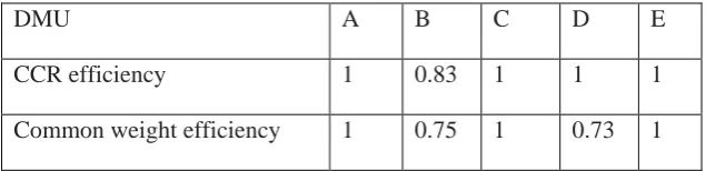
Finally, following table gives CCR efficiency and common weight efficiency values with nonlinear virtual inputs/outputs assumption for each DMU.

Table 2:

Efficiency score

E D

C B

A DMU

1 1

1 0.83 1

CCR efficiency

1 0.73 1

0.75 1

Common weight efficiency

5 Conclusion

This paper presents a common weight model with nonlinear virtual inputs/outputs assumption. Firstly, the DEA models with nonlinear virtual inputs/outputs were introduced. Then common weight models have been introduced. Finally, we proposed the common weight model with nonlinear virtual inputs/outputs based on the combination of these two concepts.

[1] Belton V and Vickers SP . Demystifying DEA-A visual interactive Approach based on multiple criteria analysis. J Opl Res Soc 44 (1993): 883-896

[2] Chen, Y-W. Larbani, M. Chang, Y-P.Multiobjective data envelopment analysis. . J Opl Res Soc (2009) 60: 1556-1566[13] Cook, W.D., Zhu, J., 2009. Piecewise linear output measures in DEA. European Journal of Operational Research 197, 312–319

[3] Cook, W.D., Yang, F., Zhu, J., 2009. Nonlinear inputs and diminishing marginal value in DEA.Journal of the Operational Research Society.doi:10.1057/jors.2008.121.

[4] Cooper, W., Seiford, L., Kaoru, T., 2006. Data Envelopment Analysis: A Comprehensive Text with Models, Applications, References and DEA-Solver Software. Springer, NY.

[5] Despotis, D.K., Stamati, L.V.,Smirlis,Y.G., 1990. Data envelopment analysis with nonlinear virtual input and outputs. European Journal of Operational Research 202, 604–613

[6] - Doyle J .Multiattrbute choice for the lazy decision maker: Let the alternatives decide. Organ Behav Hum Decis Process 62: (1995): 87-100

[7] Kao C and Hung CT . Data envelopment analysis with common weight: The compromise solution approach. J Opl Res Soc (2005) 56: 1196-1203

[8] Li X-B and Reevese GR . A multiple criteria approach to data envelopment analysis .Eur J Opl Res 115 (1999): 507-517

[9] Roll Y and Golany B . Alternative methods of treating factor weights in DEA. Omega 21 (1993): 99-103.