Please cite this article as: A. Zarei, H. Khademi Zare, M. Nakhaei Nejad, Integration of Multi-period Vehicle Routing Problem and Economic Selection of Customers with the Objective of Optimizing Distribution, Sales and Discounts Planning, International Journal of Engineering (IJE), TRANSACTIONSC: Aspetcs Vol. 29, No. 12, (December 2016) 1704-1716
International Journal of Engineering
J o u r n a l H o m e p a g e : w w w . i j e . i rIntegration of Multi-period Vehicle Routing Problem and Economic Selection of
Customers with the Objective of Optimizing Distribution, Sales and Discounts
Planning
A. Zareia, H. Khademi Zare*b, M. Nakhaei Nejada
a Department of Industrial Engineering, Faculty of Engineering, University of Science and Art, Yazd, Iran b Department of Industrial Engineering, Faculty of Engineering, Yazd University, Yazd, Iran
P A P E R I N F O
Paper history: Received 19 June2016
Received in revised form 17 September 2016 Accepted 30 September 2016
Keywords: Vehicle Routing
Economic Selection of the Customers Discounts
Collection Period Optimization
Distribution and Sales Planning
A B S T R A C T
Making decisions about the economic selection of the customers plays a significant role in the sale and logistic management of the companies. Furthermore, another issue affecting the relationship between the suppliers and the customers is the proper and timely distribution of the products as well as the optimum mixing of the distribution routes to reduce transportation costs. In this paper, the issues of the integration of routing, and the economic selection of customers has been explored aiming at minimizing the transportation, maintenance, and discount costs and maximizing the products selling profits. In addition, to the amount of customer's purchasing, costumers' collection period is effective to offer them discounts. The economic customers are selected due to three factors: the discount on the price of the product, the marginal profit of the requested products, and the distance from the supplier's warehouse. Games software was used for the exact solution of the model, and Simulated annealing algorithm was used to solve the model in larger dimension. The efficiency and applicability of the proposed model was approved comparing the optimum results with a high preciseness as 98.91 percent. Moreover, in the case study of Kalleh Company, the results revealed 14% increase in pure profits.
doi: 10.5829/idosi.ije.2016.29.12c.09
1. INTRODUCTION1
Selecting the proper set of customers and having continuous relationship with them is important and vital for a company to be successful. The main objective of the customers’ selection process is to reduce the risk of sales, maximize the overall sales value, and develop long-term relationships between customer and supplier. Choosing appropriate customers can significantly decrease distribution, sales, and discounts costs and increase the competitive capabilities of the organization. Furthermore, vehicle routing problem arises to reduce the transportation cost and increase customer's satisfaction from the proper and timely distribution of the products. The vehicle routing problem arises, in many companies, while the goods should be transported
1*Corresponding Author’s Email: [email protected] (D. Khademi
Zare)
from the suppliers to the customers [1]; so that, the reduction of the transportation costs plays an important role in reducing the total price.
transportation costs, maintenance of the inventory in the stock, increase in the profits of selling various products, and the capacities of the vehicles and warehouse, separately. However, we need an operational mathematical programming model with controllable complexity that considers all the above-mentioned cases together. In this paper, a mixed integer linear programming model is proposed for the integration of multi-period vehicle routing problem as well as the selection of the economic customers aiming at reducing the transportation and maintenance costs and increasing the benefits of selling the products. Moreover, to be more realistic, while selecting the customers, the marginal profits of the requested products and the payment period were taken into consideration besides the amount of the purchased products and the costomers’ distance from the warehouse.
In the second section of paper, a review of literature on routing, the economic selection of the customers, the discount on the price, the decrease in transportation and maintenance costs, and the increase in the profitability have been presented. The third section includes the definition and the hypotheses that are concerned with the problem as well as the related mathematical model. In the fourth section, to ensure the efficacy and applicability of the model and clarify its meaning, a small sample of the problem is taken into consideration and the effect of the priority of the intended functions on the optimal results is examined. In the fifth section, the steps of SA algorithm and the methods of codification of the answers are expressed. The sixth section shows the applicability of the proposed method using several real problems in different dimensions. In the seventh section, a case study is provided. Finally, the results of the study are explained in section 8.
2. LITERATURE REVIEW
Bakal et al. [2] established new dimensions in supply chain planning problems assuming that an inventory planning model, instead of having a specific definite or probable request, can have some demands from different markets or customers. This model includes the selection of appropriate markets and customers from the available requested basket. Geunes et al. [3] , in their first study, in areas of simultaneous market selection and production planning, explored a model in which, a manufacturer, in the single phase production, encounters some demands from the customers that he can optionally choose or reject them. Rabbani et al. [4] studied (VRP) with multi middle depots and one origin depot. In which, distribution costs are minimized and the freshness of the products delivered to the customers and the expected total profit are maximized simultaneously in one objective. In the proposed model, some customer may not receive the service because of
reducing costs. Padasht et al. [5] proposed a model which has a three-level supply chain problem consists of suppliers, distribution centers and damaged areas. The objective is to determine a few relief distribution centers between candidate areas to minimize total costs. Zabihi et al. [6] developed a hybrid MCDM method for evaluating and selecting the marine container transshipment hub port. By using the results of this research, managers of shipping lines will be able to identify the Iranian conatiner hub port and then make more precise decisions in determinining the most cost effective voyage loop for their liners. Geunes et al. [7] presented a planning model of multi-period needs with a limited time period, in the single phase production, with some constraints in production capacity, and with a mixed integer programming formulation to express the relationship between the pricing of the product and making decisions about acceptance or rejection of the demands. Over the recent years, attention has been paid to multi-objective vehicle routing. The amount of goods transported in each route, the number of the customers transported in each route, the length of the paths, and the time needed for crossing the paths are among the objectives explored in these studies [8].
Ballou [9] estimated that the costs of maintaining the inventory in any situation, over a year, are 20-40% of the total value of inventory. However, the maintenance of the inventory is necessary to increase the level of service provision to the customer and reduce the supply and distribution costs. However, managing these inventories in a scientific way to keep a minimum inventory causes the reduction in total costs. Apte and Viswanathan [10] express that over 30% of goods price is incurred in distribution process. Thus, the efficient solution on inventory control and distribution management is a vital success factor for companies [11, 12]. Hua et al. [13] by exploring the discount and transportation costs in newspaper seller problem with random demand optimized the sale's price of the product and purchase quantity of the retailers simultaneously. The obtained results showed that having some discount in transportation costs, encourages the retailers to increase their purchases in each period to reduce the total price of the goods for the customer. Setak et al. [14] assumed a firm tries to determine the optimal price, vehicle route and location of the depot in each zone to maximise its profit.
They solved the model by genetic algorithm. Moreover, Lee et al. [17] explored the model considering the price with it’s detailed and general discount. In another similar study, Fereiduni et al. [18] presented a p-robust model for humanitarian logistics in emergency situations to minimize unsatisfied demands, the government’s total cost and the suppliers’ shipping costs, when the government of the affected area declines offers of aid from international organizations because of political constraints.
A review of the literature indicates that extensive research has been done in the area of vehicle routing and selection of the customers, separately; however, in the literature, there is no simultaneous investigation of these two issues aiming at reduction in the costs of transportation, the cost of maintenance of the inventory, transportation costs, discounts, and increase in the profits.
One of the key issues in the marketing (sales) and distribution organizations is the timely payment of the customers, because, normally, in high volume purchases, the customers do not pay in cash for the purchased products. Therefore, the money of the company will remain with the customers for some times. By increasing the collection period of the customers’ receivables, the profit of the organization reduces. According to the above mentioned studies, this issue has not been studied as a factor influencing the right choice of the customers. Moreover, in the marketing organizations, discounts are considered to be part of the Sale Costs. Thus, one of the strategic objectives of the senior managers is to control the discounts offered to the customers and prevent unnecessary discounts in order to control the ratio of the prices to sales in the organization. Therefore, consideration of discounts offered to the customers as an influential factor in the selection of the customers is one of the innovations of this article. In the issues concerned with the sale and distribution of multi-products, one of the concerns of the organization is the increase in the profit margins. Different products have different profit margins. Therefore, the optimal combination of different products aiming at an increase in the profit of the organization has not been considered as a factor influencing the selection of customers in any of the studied articles.
In this paper, the issue of joint optimization of the planning of the distribution, marketing (sales), and discounts of multi-products in multi-periods have been explored in the issue of vehicle routing. To this end, a mixed-integer linear programming model is provided to have a simultaneous selection of the customers and vehicles routing. The collection period of the customers’ receivables, the marginal profit of company , requested discounts, and distance from the supplier warehouses is considered as the factors influencing the choice of customers.
3. MATHEMATICAL MODEL
The integration of the economic selection of the customers and routing policies reduces the costs of the total system, considering the value of the currency. In this study, the last level of the supply chain, i.e. the sales branch of the organization, is taken into consideration. The supplier intends to collect the customers’ orders for several future periods and design a selling plan for the products. The planning periods could be weekly, monthly, and so on. The orders are definite. If the orders are less than the goods stored in the warehouse, the goods will be maintained in the supplier’s warehouse. The capacity of the supplier’s warehouse is fixed and specified from the beginning. The inventory is considered to be zero at the beginning of the first planning period, and the inventory at the end of each period will be transferred to the next period. The suppliers offer an m × n discounts level to encourage the customers to buy more, and each customer can invest merely in one discount level. Giving discounts to the customers is based on their amount of purchasing and their collection period. The seller does not have to send the products to all of the customers. He can select them based on the costs and the benefits they impose to the company. The capacity of the vehicles sent by the seller is limited, and the seller can use the vehicles with different capacities.
3. 1. The Parameters of the Model i : index of customers (i=0,1,2,…,I)
m : index of discounts levels for the quantity of purchasing (m=1,2,…,M)
n : index of discounts levels for the customer's collection period (n=1,2,…,N)
t : index of planning period (t=1,2,…,T) v : index of vehicle (v=1,2,…,V)
k : index of the type of product (k=1,2,…,k) gt : The largest storage capacity in period t
hkt : cost of maintaining the inventory of the product,
type k, in period t
rk : price of one unit of the product, type k
yk : marginal benefits of one unit of the product, type k
dikt : order of customer i for product k in period t
cij : cost of travel from node i to node j
fv : set up or application cost of the vehicle v
cv : capacity of vehicle v
bm : the lowest amount of discount span m for the price
pm : the highest amount of discount span m for the price
an : the lowest amount of discount span n for the price
wn : the highest amount of discount span n for the price
Oikt : collection period for customer i to buy the product
type k in period t
eimnkt : the Discount percent given to the customer i for
skt : quantity of the offers of the product type k in period
t
αj : weight of the target function j
3. 2. The Decision Variables
xijvt : If vehicle v travels from the customer i to the
customer j in period t, this variable is equal to one and otherwise it is zero.
Ikt : the inventory of the product type k at the end of
period t
qinkt : If the collection period of the customer i in period
t is in discount span n, the variable is equal to one and otherwise it is zero.
Limkt : If the demand of the customer i in period t is in
discount span m, the variable is equal to one and otherwise it is zero.
ujimnvkt = qinkt * xijvt *Limkt (This binary variable was
added to linearize the model)
yi : auxiliary variable to eliminate the sub tour
3. 3. The Mathematical Model of the Problem
1 1
Max . z Min .2z23.z3 (1)
1
0 0 1 1 1
0 1 1 1 1 1 1
1 1
. . .
. . .
.
I J T V K
ijvt ikt k k
i j t v K
I M N T J V K
jimnvkt imnkt ikt k
i m n t j v k
T K
kt k
t k
z x D Y r
u e D r
S r
(1-1) 2 00 0 1 1 0 1 1
.
I J T V I V T
ij ijvt v jvt
i j t v i v t
z c x f x
(1-2)3 1 1 . T k kt kt t k
z h I
(1-3)kt 1
1 1 1 1 1 1 1
. s
K I I V K K K
kt ikt ijvt kt
K i j v K k K
I D x I
t=1,2,…,T (2) 1 1 1 . . ; M Mimkt m ikt imkt m
m m
L b D L b
i=1,2,…,I t=1,2,…,T K=1,2,…,K
(3)
1
1 1
. . ;
N N
inkt n ikt inkt n
n n
q a O q a
i=1,2,…,I t=1,2,…,T K=1,2,…,K
(4) 1 1; M imkt m L
i=1,2,…,I t=1,2,…,T K=1,2,…,K
(5) 1 1; N inkt n q
i=1,2,…,I t=1,2,…,T K=1,2,…,K
(6)
1 (1 )
1 (1 )
1 (1 )
3* ;
jimnvkt inKt imKt ijvt
jimnvkt ijvt imKt inKt
jimnvkt imKt ijvt inKt
jimnvkt inKt imKt ijvt
u q M l M X
u X M l M q
u l M X M q
u q l X
i=1,2,…,I m=1,2,…,M n=1,2,…,N t=1,2,…,T K=1,2,…,K v=1,2,…,v j=1,2,…,J
(7)
1 1 1 .
I K I
ikt jivt
i K j
D x cv
t=1,2,…,T v=1,2,…,V
(8) 1 1; I ijvt i x
t=1,2,…,T v=1,2,…,V J=1,2,…,J
(9) 1 0 0; I J ipvt pjvt i j x x
p=1,2,…,I t=1,2,…,T v=1,2,…,V
(10)
0
1 0, 1
;
I J J
ijvt jvt
i j j i j
x M x
t=1,2,…,T v=1,2,…,V
(11) 1 1 1 I V ijvt i v x
j=1,2,…,I t=1,2,…,T (12)
* ijvt 1;
Y iY jM X M
i=1,2,…,I t=1,2,…,T v=1,2,…,v j=1,2,…,J (13)
0Ikt gkt; t=1,2,…,T (14)
, Integer; , , , 0,1
, , , , , ,
i t ijvt imkt inkt jimnvkt
y I x l q u
i j v m n k t
(15)
3. 4. Introducing the Target Functions of the
Multi-product Problem The target function, in
profit of selling the products and minimize the purchasing and discount costs. The second part of the target function (1-2), which has been used to reduce the number of vehicles and distances, demonstrates the travel costs. The third part of the target function (1-3), tries to minimize the maintenance costs of the products that remain in the stocks, at the end of the period.
3. 5. Introducing the Limitations of the Model Limitation (2), in each planning period, estimates the offer of the intended period, based on the inventory remaining at the end of the previous period and the amount of production in the same period. If the total numbers of orders are more than the estimated offer in the intended period, the model omits the non-economic customers considering other limitations until the offer become equal to/greater than the total orders. Limitation (3) limits the amount of the orders at every price level to the upper and lower limits of that level. Limitation (4) limits the collection period at every collection level to the upper and lower limits of that level. Limitation (5) ensures that, in each period, each customer must receive the service at just one level of the offered discounts. Limitation (6) ensures that, in each period, the collection period for each customer must be just in one level of the offered discounts. Limitation (7) is the Linearization constraint. Limitation (8) states that the total demands of the customers in a path should not exceed the capacity of the vehicle allocated to that path. Limitation (9) states that each vehicle, in each period, should enter from maximum one node to the target node. Limitation (10) ensures that, in each period, if a vehicle enters a node, it must get out of it. Limitation (11) states that if the vehicle is going to switch between two nodes, it should, first, get out of the supplier's warehouse. Limitation (12) states that, in each period, it is just possible to enter the intended node from just one node and with just one vehicle. Limitation (13) is the sub tour elimination restriction. Limitation (14) states, in each period, it is not possible to store the goods over the storage capacity of the warehouse. Limitation (15) defines the binary and integer variables of the problem.
4. NUMERICAL EXAMPLE
In this section, in order to ensure the proper function of the model and clarify its meaning, a small sample of the problem will be examined. Then, solving the model will be explored by a meta-heuristic method; and the results of the solution will be compared, using the exact method and the meta-heuristic algorithm. For this purpose, suppose that the director of the supply section of a company decides to select from 10 customers who have ordered to the company, he should take into consideration the limitations in the offering of the
products, payment conditions, the quantity of the orders, and also their distance from the warehouse. Moreover, he should select the customers who can reduce the transportation, discount, and maintenance costs of the product being stored in the stock and increase the profits of selling products, for a 2-month planning period. The company supplies three products with different prices and different marginal profits. Table 1 reveals the price, marginal profit, and offering of each product, in each period. The offering of the products in various periods, is different. It is in such a manner to be possible to evaluate its impact on the maintenance cost of the products.
The seller has 2 vehicles to provide some services to the customers, in each period. The capacity of the first vehicle is 140 units, and the capacity of second one is 120 units. The cost of starting up for the vehicles is fixed, in each period, and the cost, for the first vehicle, is equal to 10 currency units and for the second one equal to 8 currency units. The maintenance cost is 2 currency units per each unit of the goods. Moreover, the capacity of the warehouse is fixed and equal to100 units, in each period.The customers’ distances from each other and the central depot are taken into consideration in a symmetric manner.
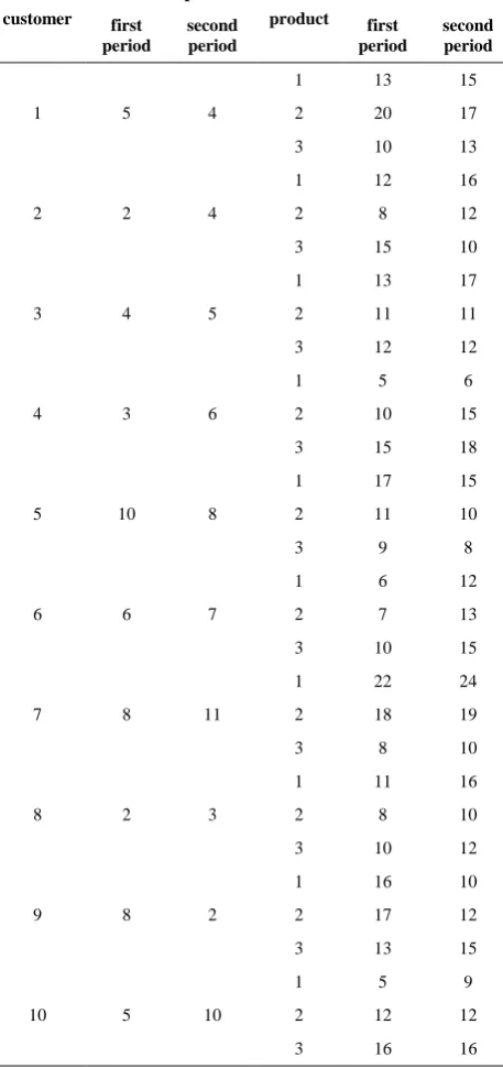
In Table 2, the orders and the collection period of each customer, in different periods, are proposed. For customers with higher average orders, higher collection period is considered. Therefore, the model can select the best customers both in terms of their orders and in terms of their collection period.
The suppliers consider three levels of discounts for the quantity of purchase and three levels of discounts for the duration of payment to encourage the customers to buy more quantity of the product and pay it in less time span. Thus, each customer will be faced with 9 levels of discounts. This means that if the customer's order is at m discount level and the collection period of the customer is at n discount level, then the customer can get e percent of discount. Discount intervals are shown in Table 3.
In this paper, GAMS22.2 linear programming software package is used to solve the problem. The mixed-integer programming optimization Packages like Gams can reach the general optimal answer or guarantee the answers with acceptable relative optimality gap.
TABLE 1. Price, margin of product and offer of each product
in each period
product price
(currency unit)
margin (percent)
offer of first period
offer of second period
1 3 1.07 95 100
2 4 1.03 90 90
TABLE 2. Demand and collection period of customers in different periods
customer
collection period
product
demand
first period
second period
first period
second period
1 5 4
1 13 15
2 20 17
3 10 13
2 2 4
1 12 16
2 8 12
3 15 10
3 4 5
1 13 17
2 11 11
3 12 12
4 3 6
1 5 6
2 10 15
3 15 18
5 10 8
1 17 15
2 11 10
3 9 8
6 6 7
1 6 12
2 7 13
3 10 15
7 8 11
1 22 24
2 18 19
3 8 10
8 2 3
1 11 16
2 8 10
3 10 12
9 8 2
1 16 10
2 17 12
3 13 15
10 5 10
1 5 9
2 12 12
3 16 16
The inputs in this model include: the demand of the customers, the customer's collection period, the cost of transportation from depot to the customer and from a customer to another customer, the offer of each product in each period, the number of the vehicles in different types, the capacity of each type of the vehicles, the start up costs of any vehicle, the vendor's storage capacity, the number of the periods, the discount levels, the price and the marginal profit of any kind of product. The outputs of the model include: the selected customers in
each period to send the goods to them and the quantity of their purchase, the number of the required vehicles of any kind, the optimal route for shipping, identification of the point that which type of vehicle with what capacity should move towards which customers, the total distribution, discounts, and maintenance costs, the quantity of each type of product being sold, and the profits obtained from selling the products.
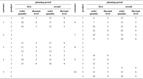
The results obtained by solving the model by Gams software are shown in Tables 4 and 5. Table 4 specifies the route of the vehicles in each planning period. Table 5 shows the number of the goods sold from each discount level in each planning period.
TABLE 3. Discounts level
discount level
demand (Dimt)
collection period
(oint)
discount percent (eimnt)
discount parameter
1 0 < D <7 & 0 < O <3 0% ei11
2 0 < D <7 & 3 ≤ O <9 0% ei12
3 0 < D <7 & O ≥ 9 0% ei13
4 7 ≤ D
<14 & 0 < O <3 1.5% ei21
5 7 ≤ D
<14 & 3 ≤ O <9 1% ei22
6 7 ≤ D
<14 & O ≥ 9 0% ei23
7 D ≥ 14 & 0 < O <3 2% ei31
8 D ≥ 14 & 3 ≤ O <9 1.5% ei32
9 D ≥ 14 & O ≥ 9 0% ei33
TABLE 4. Shipping route of vehicles
ro
w from
customer
to
customer vehicle
planning program
first second
1 i0 j4 v2 1
2 i0 j6 v2 1
3 i0 j7 v1 1 1
4 i4 j9 v2 1
5 i7 j3 v1 1
6 i7 j6 v1 1
7 i6 j10 v1 1
8 i6 j10 v2 1
9 i9 j1 v2 1
10 i10 j3 v1 1
11 i10 j4 v2 1
12 i3 j1 v1 1
13 i1 j0 v1 1
14 i1 j0 v2 1
15 i3 j0 v1 1
The results indicate that the customers 1, 3, 4, 6, 7, 9 and 10 are selected in the first period in such a way that the vehicle 1 gets out of the warehouse and goes, respectively, toward the customers 7, 6, 10 and 3, and finally returns to the warehouse. On the other hand, the vehicle 2 gets out of the warehouse and goes, respectively, toward the customers 4, 9 and 1, and finally returns to the warehouse. In the second period, the customers 1, 3, 4, 6, 7 and 10 are selected. The process is in such a way that the vehicle 1 gets out the the warehouse and goes, respectively, toward the customers 7, 3 and 1, and finally returns to the warehouse. On the other hand, the vehicle 2 gets out of the warehouse and goes, respectively, toward the customers 6, 10 and 4, and finally returns to the warehouse.
In order to explore the effect of the priority of the target functions on the optimal results, seven different ways of priority determination of the target functions will be studied. The target function is considered as the gross profit, minus the transportation and maintenance costs. It is worth noting that the gross profit includes the income gained from selling the products, minus the cost of purchasing the products and the discounts cost.
Table 6 shows that the customers who are selected and the number of them are different based on the priorities of the target functions in each problem. The model selects the customers and the best routes for them in the planning stage, counterbalancing and considering the priority of the target functions.
According to the results of Table 6, it can be considered that when it is intended to reduce the maintenance costs, the customers that have much larger orders and will result in more sales will be selected.
In the problem 3, the goal is merely to maximize the gross profit (selling revenue minus the costs of purchasing and discounts). The best policy, in these problems, is to have larger order sizes with greater marginal profit. The variations in the target functions in order to create a balance between seven problems, mentioned above, are shown in Figure 1. Figure 1 shows that, if the maintenance costs are disregarded, these costs will increase severely, and even they will be equal with the shipping costs. It is obvious in the problems 2, 3 and 5. Comparing the problems 2 and 3, the importance of paying attention to the transportation costs is highlighted. This figure also shows that paying attention to the transportation costs can reduce the total cost, almost as much as the costs of purchasing and discounts.
The minimum pure profit is related to the problem 6, in which the buyers merely pay attention to the costs of purchasing the product, discount, and maintenance. In the problem 5, the simultaneous attention to the transportation, purchasing, and discounts costs as well as the marginal profit can increase the pure profit significantly. The optimum solution will be obtained when all the costs are taken into account, equally (problem 7).
TABLE 5. Amount of the goods sold from each discount level in each planning period
cu
st
o
m
er
p
ro
d
u
ct
planning period
cu
st
o
m
er
p
ro
d
u
ct
planning period
first second first second
order quantity
discount level
order quantity
discount level
order quantity
discount level
order quantity
discount level
1
1 13 5 15 8
6
1 6 2 12 5
2 20 8 17 8 2 7 5 13 5
3 10 5 13 5 3 10 5 15 8
2 1
7
1 22 8 24 9
2 2 18 8 19 9
3 3 8 5 10 6
3
1 13 5 17 8
8 1
2 11 5 11 5 2
3 12 5 12 5 3
4
1 5 2 6 2
9
1 16 8
2 10 5 15 8 2 17 8
3 15 8 18 8 3 13 5
5 1
10
1 5 2 9 6
2 2 12 5 12 6
TABLE 6. Numerical results for balancing due to the weight of the objective function on various problems
problem 1 2 3 4 5 6 7
gross profit 532 690 752 528 700 552 570 transportation costs 330 260 320 300 270 345 300 maintainance costs 66 320 313 95 285 102 120 target (pure profit) 136 110 119 133 145 105 150
0 100 200 300 400 500 600 700 800
1 2 3 4 5 6 7
gross profit transportation costs
maintainance costs target (pure profit)
Figure 1. The objective function changes to create a balance
between seven problems
In general, we can say that to reduce the price of the goods or services and increase the satisfaction in the customer, a logical exchange between different costs should be established.
In the problem 2, the goal of which is to minimize the transportation costs, the determiner must reduce the number of transports and select the customers with larger order size and lower distance from the warehouse to reduce the number of the vehicles used and the distance traveled. In the problem 3, in which the determiner's attention is focused on the marginal profit of the customer's demand, the supplier gets confused. This is because of the fact that when the customers with higher marginal profit in their overall demands are selected, the gross profit increases, but the pure profit decreases sharply. Thus, the results of excessive attention to the marginal profits of the product and inattention to the cost of transportation can be revealed clearly. The results show that considering all the target functions can increase the pure profit 21%, as an average, compared with the time when only some of them are taken into consideration. It seems that the best ordering policy can be achieved by paying attention to all the costs together, because inattention to one of the costs causes the increase in the costs and decrease in the final profit.
5. THE SA PROPOSED SOLUTION
The VRP problem is among the NP-hard problems that require the innovative approaches to solve it in
large-scale [19]. Therefore, an efficient meta-heuristic algorithm based on simulated annealing (SA) is proposed. This algorithm works efficiently on a neighborhood search within the solution space. Moreover, one of the advantages of this algorithm is that it can escape from being trapped in local optima and move toward the target function [20].
The basic steps of the proposed SA algorithm are shown in Figure 2. Before mentioning the steps of SA algorithm, we initially define the input parameters of the problem:
EL = the length of Markov chain (the number of the accepted answers, in each temperature, or the criteria of going out of the inner ring).
MTT = Maximum transitions in the temperature (Stopping the algorithm or the criteria of going out of the inner ring).
T0 = The initial temperature
α= Temperature reduction coefficient X = Feasible solution
C(X) = the target function value for feasible solution. M = the counter counting the number of the accepted answer at any temperature.
K = the counter counting the number of the temperature transmissions
5. 1. The Algorithm Producing the Initial Solution Producing the initial solutions is the first step in any meta-heuristic approach. In order to produce the initial solution, the following innovative approach is used:
1. The formation of the new route: select a car (like v) from the available vehicles, by chance, and send it towards a customer (the customers that their total orders for all the products are not more than the capacity of the vehicle).
2. Determining the neighboring nodes: find the closest node to the node i (such as node j) in a way that their total orders for all the products are not greater than the remaining capacity of the vehicle. If such a node is found, send the car v from the node i to j; Otherwise, send it back to the warehouse.
3. Route completion: Repeat the second step as many times as there remain no customers with his total orders not exceeding the remaining capacity of the car.
4. Tours completion : Then among the available cars, choose another car, randomly. And in the same way mentioned above, a random tour is created for the car. Naturally, the customers who have received the services by the previous car, in the previous step, should be omitted from selection process at this step.
5. Service completion : The process of selecting the car and its corresponding tour, for the first period, continues until either all the customers are serviced or all the cars are selected.
6. When the selections for the first period finished, the same process will exactly continue for the subsequent periods. When, the cars and the corresponding tours are selected for all of the periods, the first stage of producing the initial answer is finished.
5. 2. Modifications The answer produced
according to the stages mentioned above, may be unjustified. That can be the result of overstepping from the source (the amount of production in each period). So at this stage, the initial answer will be modified.
For all the periods and in each period for all the machines that are used in the same period, the following process is done:
Exploring the Limitations in the Capacity of the Car: If the capacity of the car is violated, select a customer from the corresponding tour of the car, randomly, and omit it. The random selection and omission of a customer from the tour should be continued until the capacity of the car isn’t violated.
Exploring the Limitations in the Produced Recourses: First, check whether it is possible to provide services to the customers selected for the first period, according to the amount of production, in the same period. If this is not possible, select one of the cars used in the first period, randomly, and select a customer from the corresponding tour by chance, and omit it. Selecting a vehicle and a customer from the corresponding tour, continued until the picked customers could be serviced, due to the production constraints. Then, the remaining productions, move to the next period. Besides, the same activities should be done for the next period.
After producing the initial answers, the value of the corresponding target function is calculated. Calculating the target function the discount level can be calculated, considering the selected customers in each period, the orders, and the collection period of them. Regarding the tours of the cars, the transportation cost is calculated. The maintenance costs are calculated based on the inventory moved from one period to the next. According to the kind of cars used in the answer, the set-up cost of vehicles is calculated.
5. 3. How to Produce Neighborhood Six
operators are used to produce neighborhood. Each time producing the neighborhood, one of the operators is randomly selected.
The first operator: exchange two customers from two different tours: First of all, a period is chosen, randomly. Then, two cars (which have been used in that period) will be chosen by chance. A customer is selected from the tour corresponding to each vehicle. At last, the two customers are replaced with each other.
The second operator: Replacement of two customers in a tour: First of all, a period is chosen, randomly. Then, a car from the same period, is randomly selected. Next, from the tour corresponding to that car, two customers are chosen randomly and are replaced with each other.
The third operator: replacement of the vehicles: a period is chosen randomly and a car from the same period is selected by chance. Then, the selected car will be replaced with one of the available vehicles (that was not used in the answer).
The fourth operator: Shift a customer of a tour to another tour: First of all, a period is chosen randomly. Then, in that period, a car is chosen randomly and a customer from the corresponding tour of that car is selected.Then, another car is chosen from the same period. At last, the selected customer is eliminated from his previous position and moved to a random position in the tour of the second car.
The fifth operator: a period is chosen randomly. Then, a customer from the customers, who were not serviced, is chosen randomly. A car from the same period is selected. Finally, the selected customer is placed in a random position in the tour of that car.
The sixth operator: a period is chosen randomly .A customer who was not serviced in that period is chosen randomly. He is replaced with one of the customers who are served during this period. (For choosing the customer, first, a car is selected randomly and then a customer from its corresponding tour is chosen).
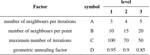
Table 7 shows the factors affecting the answer of the simulated annealing algorithm, which have been considered at three levels:
The experiments were planned based on L9 taguchi orthogonal array. All test results have been estimated in Figure 3.
As it is apparent in Figure 3, the optimal levels for the parameters are: A(2), B(2), C(1), D(1). The final configurations of the parameters for sa algorithm are represented in Table 8.
In all the represented results and the examples of the samples, the parameters have been considered as above.
6. VALIDATION OF THE MODEL
Considering the items designed in the model and the expansions in SA solving methods, a program is written using MATLAB software. Based on the proposed model and its solution using SA Algorithm, in this section, several real problems with various dimensions are selected and it is attempted to solve these problems to show the efficiency and applicability of the model comparing the results of the program written in MATLAB with the answers of Gams software.
TABLE 7. Input for simulated annealing method
Factor symbol
level
1 2 3
number of neighbours per iterations A 3 4 5 number of neighbours per point B 10 15 20 maximum number of iterations C 100 70 50 geometric annealing factor D 0.95 0.9 0.85
TABLE 8. Confirmation parameters of simulated annealing
algorithm
parameter A(2) B(2) C(1) D(1)
The optimal value 4 15 100 0.95
3 2 1 -50 -51 -52 -53
3 2 1
3 2 1 -50 -51 -52 -53
3 2 1 A
M
e
a
n
o
f
S
N
r
a
ti
o
s
B
C D
Main Effects Plot for SN ratios
Data Means
Signal-to-noise: Smaller is better
Figure 3. S/N diagram of simulated annealing
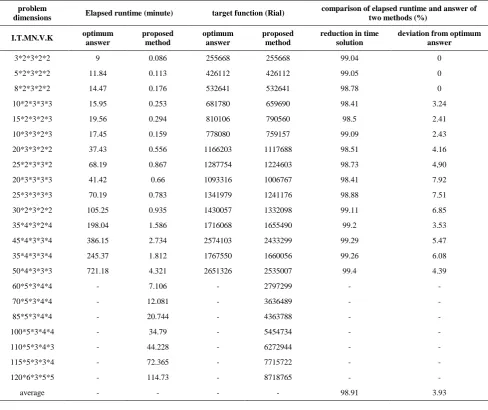
The dimensions of the problem have been determined using I.T.MN.V.K equation, in which I represents the number of the customers, T shows the number of the periods, MN reveals the number of the discount levels, V provides the number of the vehicles, and K presents the number of the products in different kinds. The target function being the profit (the revenue minus the costs of purchasing the product, discounts, shipping, and maintenance) and the time required in order to get to the answer are shown in Table 9.
Comparing the results of SA with the optimum results of Gams, it can be concluded that the software used based on the SA algorithm has the capability to come to the optimum answer while solving problems. On the other hand, estimating the time required for solving the problem in both the SA and Gams models, it is revealed that there is severe increase in the time needed for solving the problem in Gams model, while the time needed to solve the problem by SA algorithm increases slightly in high dimensions. Studing the increase in the time needed for solving the problem, the impact of increasing the variety of the products in increasing the required time could be observed. The results provided in Table 8 show that the answers of the suggested method deviate from the optimal answers 3.93 percent, as an average.
7. CASE STUDY
In order to explore the efficacy of the proposed algorithm, a real problem has been studied. The case study in this paper is Kalleh Company, one of the largest producers and distributors of dairy, meat, and drinks in Iran. The products of this company are offered to the market in more than 400 various types. Kalleh Company has a marketing representation in Shiraz. This branch sells the products to more than 2000 customers.
Providing the services to these customers is done using 20 Isuzu trucks with the capacity equal to 2000 kg and 2 Nissan trucks with the capacity equal to 1000 kg. Kalleh Company has been unprofitable in selling their products in one of the lines during some frequent months. However, there is a better solution. This company believes that some of the customers are not profitable enough, considering the costs that they impose to the company for visitors, distributor, sending the car, and etc.
TABLE 9. Comparing the resaults of SA and Gams
problem
dimensions Elapsed runtime (minute) target function (Rial)
comparison of elapsed runtime and answer of two methods (%)
I.T.MN.V.K optimum
answer
proposed method
optimum answer
proposed method
reduction in time solution
deviation from optimum answer
3*2*3*2*2 9 0.086 255668 255668 99.04 0
5*2*3*2*2 11.84 0.113 426112 426112 99.05 0
8*2*3*2*2 14.47 0.176 532641 532641 98.78 0
10*2*3*3*3 15.95 0.253 681780 659690 98.41 3.24
15*2*3*2*3 19.56 0.294 810106 790560 98.5 2.41
10*3*3*2*3 17.45 0.159 778080 759157 99.09 2.43
20*3*3*2*2 37.43 0.556 1166203 1117688 98.51 4.16
25*2*3*3*2 68.19 0.867 1287754 1224603 98.73 4,90
20*3*3*3*3 41.42 0.66 1093316 1006767 98.41 7.92
25*3*3*3*3 70.19 0.783 1341979 1241176 98.88 7.51
30*2*3*2*2 105.25 0.935 1430057 1332098 99.11 6.85
35*4*3*2*4 198.04 1.586 1716068 1655490 99.2 3.53
45*4*3*3*4 386.15 2.734 2574103 2433299 99.29 5.47
35*4*3*3*4 245.37 1.812 1767550 1660056 99.26 6.08
50*4*3*3*3 721.18 4.321 2651326 2535007 99.4 4.39
60*5*3*4*4 - 7.106 - 2797299 - -
70*5*3*4*4 - 12.081 - 3636489 - -
85*5*3*4*4 - 20.744 - 4363788 - -
100*5*3*4*4 - 34.79 - 5454734 - -
110*5*3*4*3 - 44.228 - 6272944 - -
115*5*3*3*4 - 72.365 - 7715722 - -
120*6*3*5*5 - 114.73 - 8718765 - -
average - - - - 98.91 3.93
TABLE 10. Comparing the results of the proposed method
and the current status in case study
Pure profit serving time solution time
(currency unit) (minute) (second)
proposed method 5854584 1072/344 2/061
existing condition 4404214 1320 -
During this period, the company not only loses the benefits from the circulation of the money, but also is obliged to borrow some money from the bank to cover its operating costs. Another issue is related to the inopportune discounts that are given to the customers only because of customer's insistence, regardless of various factors. If the discounts could be controlled, it would prevent a large number of additional costs. The next factor is concerned with the lack of inclusion of the
transportation and maintenance costs at this decision. Therefore, according to the needs of the company in proper selection of the economic customers, the proposed model was designed and applied in the company. This study is conducted on the data obtained from the purchases of the customers in the past 36 months. In this research, a crossroads, in the middle of the target area, was selected as the origin of the coordinates. Then, the characteristics of the customers and the depot were determined based on that origin. It is clear from the first planning period that how much product should be sold to which customers, in each period. In addition, it is determined that the vehicles should choose which routes to move toward the customers, taking into consideration their capacities.
specifications Corei3 cpu2.13 GH and a memory equal to 4GB RAM. The responses obtained from the proposed method have been compared with the existing data from the current method, and the results are represented in Table 10.
As the results reveal, applying the proposed model, in this company, resulted in 14% increase in the pure profit of selling. Besides, the availability of the specified optimized routes to move from the depot to the customers resulted in some reduction in the time spent for service provision.
8. CONCLUSION
In this study, it is attempted to propose a method to joint optimization of the planning of the distribution, marketing, and discounts of products in multi-periods in the issue of vehicle routing. In order to simultaneous selection of the customers and vehicles routing, a mixed integer linear programming model was designed to minimize the transportation, maintenance, and discount costs and maximize the profits obtained from selling the products. To expand the proposed model, the discount given to each customer was taken into consideration based on the quantity of his purchase and the collection period. In addition, the type of the products that the consumers purchase and the marginal profit has been involved in the selection of the customers. For the exact solution of the model, Gams software is used, and for solving it in larger dimensions, the simulated annealing algorithm is used. The applicability of the proposed method is examined in a case study and several problems with different dimensions. The application of this method at Kalleh Company, in Shiraz, caused 14 percent increase in the profit and no delay in the process of service provision by proper selection of the economic customers and the optimum routes. Comparing the answers provided by SA algorithm, with the optimum solutions, 3.93 percent deviation, in average, was observed. However, the time needed for coming to the intended results, in this way, reduced at least 98% compared to the ones obtained using Gams software. Further research can be done (improving this method) considering the limitations in time spans for sending and receiving the goods, the costs of shortcomings in the target function, and multi-depot instead of one multi-depot. This model can be improved entering the fuzzy or probable parameters in the model.
9. REFERENCES
1. Sohrabi, B. and Bassiri, M., "Experiments to determine the simulated annealing parameters case study in vrp", International Journal of Engineering Transactions B, Vol. 17, No. 1, (2004), 71-80.
2. Bakal, I. S., Geunes, J. and Romeijn, H. E., "Market selection decisions for inventory models with price-sensitive demand", Journal of Global Optimization, Vol. 41, No. 4, (2008), 633-657.
3. Geunes, J., Shen, Z.-J. and Romeijn, H. E., "Economic ordering decisions with market choice flexibility", Naval Research Logistics, Vol. 51, No. 1, (2004), 117-136.
4. Rabbani, M., Farshbaf-Geranmayeh, A. and Haghjoo, N., "Vehicle routing problem with considering multi-middle depots for perishable food delivery", Uncertain Supply Chain Management, Vol. 4, No. 3, (2016), 171-182.
5. Padasht, S. and Razmi, J., "A location-routing model on relief distribution centers", Uncertain Supply Chain Management, Vol. 4, No. 4, (2016), 269-276.
6. Zabihi, A., Gharakhani, M. and Afshinfar, A., "A multi criteria decision-making model for selecting hub port for iranian marine industry", Uncertain Supply Chain Management, Vol. 4, No. 3, (2016), 195-206.
7. Geunes, J., Romeijn, H. E. and Taaffe, K., "Requirements planning with pricing and order selection flexibility", Operations Research, Vol. 54, No. 2, (2006), 394-401. 8. Lee, T.-R. and Ueng, J.-H., "A study of vehicle routing problems
with load-balancing", International Journal of Physical Distribution & Logistics Management, Vol. 29, No. 10, (1999), 646-657.
9. Ballou, R. H., "A multiproduct plant/warehouse location model with nonlinear inventory costs", Journal of Operations Management, Vol. 5, (1975), 75-90.
10. Apte, U. M. and Viswanathan, S., "Effective cross docking for improving distribution efficiencies", International Journal of Logistics, Vol. 3, No. 3, (2000), 291-302.
11. Wang, J.-L., "A supply chain application of fuzzy set theory to inventory control models–drp system analysis", Expert Systems with Applications, Vol. 36, No. 5, (2009), 9229-9239. 12. Fakhrzada, M. and Esfahanib, A. S., "Modeling the time
windows vehicle routing problem in cross-docking strategy using two meta-heuristic algorithms", International Journal of Engineering-Transactions A: Basics, Vol. 27, No. 7, (2013), 1113-1126.
13. Hua, G., Wang, S. and Cheng, T., "Optimal pricing and order quantity for the newsvendor problem with free shipping", International Journal of Production Economics, Vol. 135, No. 1, (2012), 162-169.
14. Setak, M., Dastaki, M. S. and Karimi, H., "Investigating zone pricing in a location-routing problem using a variable neighborhood search algorithm", International Journal of Engineering-Transactions B: Applications, Vol. 28, No. 11, (2015), 1624-1633.
15. Mirzaei, A. H., Nakhai, K. I. and Zegordi, S. H., "A new algorithm for solving the inventory routing problem with direct shipment", Journal of Production and Operations Management, (2012), 1-28.
16. Lee, A. H., Kang, H.-Y. and Lai, C.-M., "Solving lot-sizing problem with quantity discount and transportation cost", International Journal of Systems Science, Vol. 44, No. 4, (2013), 760-774.
17. Lee, A. H., Kang, H.-Y., Lai, C.-M. and Hong, W.-Y., "An integrated model for lot sizing with supplier selection and quantity discounts", Applied Mathematical Modelling, Vol. 37, No. 7, (2013), 4733-4746.
19. Potvin, J.-Y. and Rousseau, J.-M., "An exchange heuristic for routeing problems with time windows", Journal of the Operational Research Society, Vol. 46, No. 12, (1995), 1433-1446.
20. Tavakkoli-Moghaddam, R., Sayarshadand, H. and ElMekkawy, T., "Solving a new multi-period mathematical model of the rail-car fleet size and rail-car utilization by simulated annealing", International Journal of Engineering, Transactions A: Basics, Vol. 22, No. 1, (2009), 33-46.
Integration of Multi-period Vehicle Routing Problem and Economic Selection of
Customers with the Objective of Optimizing Distribution, Sales and Discounts
Planning
A. Zareia, H. Khademi Zareb, M. Nakhaei Nejada
a Department of Industrial Engineering, Faculty of Engineering, University of Science and Art, Yazd, Iran b Department of Industrial Engineering, Faculty of Engineering, Yazd University, Yazd, Iran
P A P E R I N F O
Paper history: Received 19 June2016
Received in revised form 17 September 2016 Accepted 30 September 2016
Keywords: Vehicle Routing
Economic Selection of the Customers Discounts
Collection Period Optimization
Distribution and Sales Planning
ديكچ ه نیوصت یزیگ رد درَه ةبختًا یدبصتقا ىبیزتطه صقً لثبق یْجَت رد شٍزف ٍ تیزیذه کیتسجل تکزض بّ دراد . یکی ،يیٌچوّ زگید سا تبعَضَه راذگزیثبت رد طثاٍر ىبیه يیهبت ىبگذٌٌک ٍ ،ىبیزتطه عیسَت حیحص ٍ ِث عقَه تلاَصحه ٍ تیکزت ٌِیْث سا یبّزیسه عیسَت تْج صّبک ٌِیشّ یبّ لوح ٍ لقً تسا . رد يیا ِلبقه ِث ِلئسه ِچربپکی یسبس ذٌچ ُرٍد ،یا ذٌچ یلَصحه یثبیزیسه ٍ ةبختًا یدبصتقا ىبیزتطه بث فذّ لقاذح ىدَوً ٌِیشّ یبّ لوح ٍ ،لقً ٌِیشّ یبّ یراذْگً یدَجَه رد ،ربجًا ٌِیشّ یبّ فیفخت ٍ زثکاذح ىدَوً دَس لصبح سا شٍزف ،تلاَصحه ِتخادزپ ُذض تسا . ٍُلاع زث نجح ذیزخ ،ىبیزتطه تذه ىبهس تخادزپ ىبیزتطه رد ىاشیه ِئارا فیفخت ِث بًْآ زثَه تسا . ىبیزتطه یدبصتقا بث ِجَت ِث ِس لهبع فیفخت تویق ،لابک ِیضبح دَس تلاَصحه یتساَخرد ٍ ِلصبف سا ربجًا يیهبت ُذٌٌک ةبختًا یه ذًَض . یازث لح قیقد لذه سا مزً راشفا شوگ ٍ یازث لح رد دبعثا زتگرشث سا نتیرَگلا ِیجض یسبس ذیزجت ُدبفتسا ُذض تسا . ییاربک لذه یدبٌْطیپ بث ِسیبقه ةاَج یبّ ٌِیْث بث تقد یلابث ۱۹ / ۱۹ ذصرد یه ذضبث . يیٌچوّ رد ِعلبطه یدرَه تکزض ِلبک سازیض ، جیبتً ،لصبح صّبک ۹1 یذصرد رد ٌِیشّ یبّ يیا تکزض ار ىبطً یه ذّد .