Online State Space Model Parameter Estimation in Synchronous Machines

124 Iranian Journal of Electrical & Electronic Engineering, Vol. 10, No. 2, June 2014

Online

State Space Model Parameter Estimation in

Synchronous Machines

Z. Gallehdari*, M. Dehghani**(C.A.) and S. K. Y. Nikravesh*

Abstract: In this paper a new approach based on the Least Squares Error method for estimating the unknown parameters of the 3rd order nonlinear model of synchronous generators is presented. The proposed approach uses the mathematical relationships between the machine parameters and on-line input/output measurements to estimate the parameters of the nonlinear state space model. The field voltage is considered as the input and the rotor angle and the active power are considered as the generator outputs. In fact, the third order nonlinear state space model is converted to only two linear regression equations. Then, easy-implemented regression equations are used to estimate the unknown parameters of the nonlinear model. The suggested approach is evaluated for a sample synchronous machine model. Estimated parameters are tested for different inputs at different operating conditions. The effect of noise is also considered in this study. Simulation results declare that the efficiency of the proposed approach.

Keywords: Identification, Nonlinear Model, Regression Equation, State Space Model, Synchronous Machine.

1 Introduction1

As the power system becomes more complicated and more interconnected, modeling and identification of its elements become more essential. Synchronous generators play an important role in the stability of power systems, so the accurate modeling of synchronous generators is essential for a valid analysis of dynamic and stability performance in power systems [1].

There are many different methods for synchronous machine modeling [2-4], but we can categorize all modeling techniques to three classes: white box [5-6], grey box [7-9] and black box [10-12]. The first category assumes a known structure for the synchronous machine such as the traditional methods, which are specified in IEEE and IEC standards [13]. These approaches are often conducted under off-line condition. The parameters obtained by these methods may not truly characterize the synchronous machine under various loading conditions [8].

According to the disadvantages of off-line methods, on-line parameter estimation approaches are of more

Iranian Journal of Electrical & Electronic Engineering, 2014. Paper first received 16 Jan. 2013 and in revised form 6 Oct. 2013. * The Authors are with Electrical Engineering Department, Amirkabir University of Technology, Tehran, Iran.

** The Author is with School of Electrical and Computer Engineering, Shiraz University, Shiraz, Iran.

E-mails: [email protected], [email protected] and [email protected].

interest in the recent years. The second and the third categories both use online measurements to estimate synchronous generator parameters, but they act in different ways.

In the second type of identification methods, a known mathematical model for synchronous generator is assumed and on-line measurements are used to estimate machine’s physical parameters. In the third one, input data set is mapped to the output data set without considering any known structure for the model.

In synchronous generators modeling, we have two kinds of nonlinearities. The first kind of nonlinearities is structured nonlinearities, such as sine and cosine functions of the rotor angle, which are modeled in the well-known nonlinear structures of synchronous models. On the other hand, the unstructured nonlinearities e.g. magnetic saturation in the iron parts of the rotor and stator are not usually considered in the structure of the models and instead are reflected by adjusting the physical parameters of the nonlinear model based on the online measurements [14].

In this paper, an analytical identification procedure for the 3rd order model of synchronous generators is suggested. The proposed method estimates physical parameters of synchronous machine. In [1, 9, 14-15] different algorithms for estimation of physical parameters of synchronous machine are presented. In [9] an approach for synchronous generator parameter estimation is suggested which needs to apply a short circuit on the generator terminals. This short circuit test

will disturb t a method is parameter es set of equatio solved nume discuss the c can be solve result in a sin be found. In which needs signal. This operation of not only the parameters, eigenvalues find an algor of the param In other word find a way to

In this s forward and measurement Here we onl Then, using parameters o estimated.

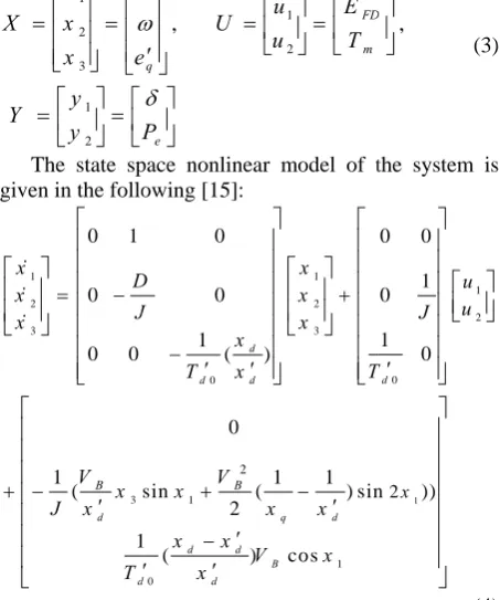
The pape generator m described in simulation re concludes th 2 The Sync

In this pa generator co the system stator’s dyn neglected, so field dynami low-frequenc power system The third is used in thi be in per un following no 1 ( 1 ( m q FD do T J e E T δ ω ω = = − ′ = ′ where:

Fig. 1 structur

the normal op s suggested f stimation, wh ons. In each te

rically. Furthe conditions in w

ed. In some ngular set of n [15], an an to perturb th s signal is n f the machine

e mathematic but also it n using the Pro rithm, which u meters and the

ds, we try to e o omit its disad tudy, we intr d easy-implem

ts to estimat ly need to so

some simpl of 3rd order no

er is organized model and th

n Sections 2 esults are pro

e paper. chronous Gen aper, the third

nnected to an under study namics and t o we have onl ic). This mod cy oscillation ms [1, 14]. d order nonlin

is paper. All t nit values. Th onlinear equati

)

( e

D q d

T D

e x x

ω −

′

− − −

re of the study s

eration of the for the synch hich results in est, the nonlin ermore, the al which the sys situations, the

equations and nalytic approa e field voltag not harmful e. The sugges cal relation b needs to iden ony approach. uses the mathe extra step of P extend the me dvantage. roduce an an mented meth te the unkno olve two regre le relations a onlinear state d as follows: he identificati 2 and 3, re ovided in Sect

nerator Mod d order nonlin n infinite bus (Fig. 1). In the effects o ly one electri del can be us ns and stabi near model de

the parameter he model is d

ions:

) ) d d

x i′

system.

machine. In [ hronous mach n some nonlin near set should lgorithm does stem of equati e algorithm m d no solution ach is sugges

e with the PR for the norm sted method u between mach ntify the syst . Here, we try ematical relati

Prony is omit ethod of [15] nalytical, strai hod, uses onl own paramet ession equatio all the unkno space model the synchron ion method espectively. T

tion 4. Sectio

el

near synchron is considered this model, of dampers cal equation ( sed for study ility analysis erived in [16-rs are assumed

described by [14] hine near d be not ions may can sted RBS mal uses hine tem y to ions ted. and ight line ters. ons. own are nous are The on 5 nous d as the are (the ying of -18] d to the (1) d q e i i T neg con i.e. the is g mo the out X Y giv x x x + ⎡ ⎢ ⎢ ⎣ ⎡ ⎢ ⎢ ⎢ ⎢ ⎢ ⎢ ⎢ ⎣ vic kno ⎡ ⎢ ⎢ ⎢⎣ x x x Y cos sin s q B d B q B e q d e V x V x V P e x δ ′ − = ′ = ′ ≅ = ′

In this mode glected, so nstant. xd,x . the line and em [15]. The d

given in the A In our study odel of the sys e state space tputs are defin

1 2 3 1 2 x x x e y y δ ω ⎡ ⎡ ⎤ ⎢ ⎢ ⎥ = _{⎢ ⎥= ⎢} ⎢ ⎢ ⎥ ⎣ ⎦ ⎣ ⎡ ⎡ ⎤ =_{⎢ ⎥= ⎢} ⎣ ⎦ ⎣

The state sp ven in the follo

1 2 3 3 0 1 0 0 0 1 ( 1 d d B x D x J x V x J x T = − − ′ ⎡ ⎢ ⎢ ⎤ ⎢ ⎥ _⎢ ⎥ ⎦ ⎢ ⎢ ⎢⎣ ⎡ ⎣ From [15], t cinity of an o

own Heffron-1 1 2 3 4 1 2 0 ⎡ ⎢ ⎢ ⎤ ⎢ ⎥ = −_⎢ − ⎥ ⎢ ⎥⎦ ⎢− ⎢ ′ ⎣ Δ ⎡ ⎡ ⎤ =_{⎢ ⎥= ⎢} Δ ⎣ ⎦ ⎣ do e K J K T y P y δ 2 ₁ sin ( 2 B q V x δ δ +

l, the influenc ,

d q

x x and q and

x

d

′

are

d transformer definition of t Appendix.

y, it is requir stem, so the ab e one. The s ned as follows

, q e U e P δ ω δ ⎤ ⎥ ₌ ⎥ ⎥ ′ ⎦ ⎤ ⎥ ⎦ pace nonlinea owing [15]: 0 1 0 2 0 0 1 ( 0 sin ( 2 1 ( ) d d d d d d d B D J x T x V x x x V x − ′ ′ + ′ − ′ ′ the linearized operating poi -Philips model 2 3 1 1 0 1 0 1 0 0 ⎤ ⎥ ⎥ ⎥ − − _⎥ ⎥ ⎥ − _⎥ ′ ⎦ ⎤ ⎡₌ ⎥ ⎢_⎣ ⎦ do K D J J K T K K 1 1 ) sin(2 q xd

δ −

′

ce of magnetic

d

x

′

are ass e the augment reactances ar the variables red to find th bove model is system states s: 1 2 FD m u E u T ⎡ ⎤ ⎡ = ⎢ ⎥ ⎢ ⎣ ⎦ ⎣

ar model of t

1 2 3 1 ) 1 1

( ) sin

cos q d B x x x T x x V x + − ′ ⎤ ⎡ ⎥ ⎢ ⎥_{⎡ ⎤} ⎢ ⎥_{⎢ ⎥} ⎢ ⎥_{⎢ ⎥} ⎢ ⎣ ⎦ ⎥ ⎢ ⎥ ⎢ ⎥ _⎢⎣ ⎦ d model of E int ‘o’, will l, which is giv

1 2 3 1 2 2 3 0 0 1 0 ⎤ ⎡ ⎢ ⎢ ⎡ ⎤ ⎢ ⎢ ⎥ +_⎢ ⎢ ⎥ ⎢ ⎢ ⎥ ⎣ ⎦ ⎢ ⎢ ′ ⎣ ⎦ ⎡ ⎤ ⎤ ⎢ ⎥ ⎥ ⎢ ⎥ ⎦ ⎢ ⎥_{⎣ ⎦} do x x x T x x K x ) δ (2)

c saturation is sumed to be ted reactance, re added with and constants he state space s converted to s, inputs and

, D⎤

⎥

⎦ (3)

the system is

1 1 2 0 2 0 0 1 0 1 0 n )) d x u u J T ′ ⎤ ⎥ ⎥ ⎡ ⎤ ⎥ ⎢ ⎥ ⎥ ⎣ ⎦ ⎥ ⎥ ⎥⎦ ⎤ ⎥ ⎥ ⎥ ⎥ ⎥ ⎥ ⎥ ⎦ (4) q. (4), in the conclude the ven below: 1 2 0 1 0 ⎤ ⎥ ⎥ ⎡ ⎤ ⎥ ⎢ ⎥ ⎥ ⎣ ⎦ ⎥ ⎥ ⎥⎦ u u J (5)

) s e , h s e o d ) s ) e e )

126 Iranian Journal of Electrical & Electronic Engineering, Vol. 10, No. 2, June 2014 where:

2 30

1 10 10

1 1

cos ( ) cos 2

B

B

d q d

x V

K x V x

x x x

= + −

′ ′ (6)

10 2

sin B

d

V x

K

x

=

′ (7)

3

d d x K

x ′

= (8)

10 4

sin

( )

B

d d d

V x

K x x

x ′

= −

′ (9)

To avoid complexity in equations, we define unknown parameters in Eq. (5) as p1, p2, …, p7. The

linear dynamical model can be written as follows:

1 2 3 7

4 5 6

3 1

7 7

0 1 0 0 0

0

0 0

1 0 0

0

A B

X p p p X p U

p p p

Y X

p p

p p

⎡ ⎤ ⎡ ⎤

⎢ ⎥ ⎢ ⎥

=_{⎢ ⎥} +_{⎢ ⎥}

⎢ ⎥ ⎢ ⎥

⎣ ⎦ ⎣ ⎦

⎡ ⎤

⎢ ⎥

⎢ ⎥

=

⎢_{− −} ⎥

⎢ ⎥

⎣ ⎦

(10)

The corresponding nonlinear model will be:

1 1

1

2 2 2 7

2

3 5 3 6

2

3 1 1

5 6 1

1 2

3 1 1

0 1 0 0 0

0 0 0

0 0 0

0

1 1 1

( sin ( ) sin 2 ))

2

( ) cos

1 1

sin sin 2

2

B B

m

d q d

d q d

x x _u

x p x p _u

x p x p

V V

T x x x

J x x x

p p V x

x

V V

y _{x x x}

x x x

⎡ ⎤ ⎡ ⎤

⎡ ⎤ ⎡ ⎤ _{⎡ ⎤}

=⎢ ⎥ +⎢ ⎥ +

⎢ ⎥ ⎢ ⎥ _{⎢ ⎥}

⎣ ⎦

⎢ ⎥ ⎢ ⎥

⎢ ⎥ ⎢ ⎥

⎣ ⎦ ⎣ ⎦⎣ ⎦ ⎣ ⎦

⎡ ⎤

⎢ ⎥

⎢ ⎥

⎢ _{− − −} ⎥

⎢ _{′ ′} ⎥

⎢ ⎥

⎢ _{− +} ⎥

⎢ ⎥

⎣ ⎦

⎡ ⎤

⎢ ⎛ ⎞

= ⎢ _′ + ⎜_⎜ − _′⎟_⎟

⎢ _{⎝ ⎠}

⎣

⎥ ⎥ ⎥⎦

(11)

Comparing the above equations, it is obvious that the linear and the nonlinear models have some common parameters, which are independent from the operating point condition. These common parameters are used to identify the nonlinear model.

3 Identification Method

In the identification methods, the signals are sampled and the samples are used to identify the model. On the other hand, the discrete equations are difference not differential type; this causes the discrete equations to be easy for implementation. Because of these two reasons, we discretize the synchronous generator model with sample time ‘h’ and use the discrete model instead of the continuous one.

The discrete model of the system in Eq. (10) is given in the following:

1 1

2 1 2 3 2

3 4 5 3

1 7

2 6

( 1) 1 0 ( )

( 1) 1 ( )

( 1) 0 1 ( )

0 0

( ) 0

( ) 0

x k h x k

x k hp hp hp x k

x k hp hp x k

u k hp

u k hp

+

⎡ ⎤ ⎡ ⎤ ⎡ ⎤

⎢ ₊ ⎥ ⎢_{= +} ⎥ ⎢ ⎥

⎢ ⎥ ⎢ ⎥ ⎢ ⎥

⎢ + ⎥ ⎢ + ⎥ ⎢ ⎥

⎣ ⎦ ⎣ ⎦ ⎣ ⎦

⎡ ⎤

⎡ ⎤

⎢ ⎥

+_{⎢ ⎢ ⎥}

⎥ ⎣ ⎦

⎢ ⎥

⎣ ⎦

(12)

1 1

2

2 1 3

3

7 7

1 0 0 ( )

( )

( ) ( )

0 ( )

x k y k

x k

y k p p

x k

p p

⎡ ⎤

⎡ ⎤

⎢ ⎥

⎡ ⎤ _{⎢ ⎥⎢ ⎥}

=

⎢ ⎥ _{⎢ ⎥⎢ ⎥}

⎣ ⎦ _{− − ⎢ ⎥}

⎢ ⎥ ⎣ ⎦

⎣ ⎦

(13)

Since our goal is to find the relation between the machine’s parameters and its outputs, we write the states in terms of the machine’s outputs.

1( ) 1( )

x k =y k (14)

1 1

2

( 1) ( )

( ) y k y k

x k

h + −

= (15)

7 1

3 2 1

3 7

( ) p ( ( ) p ( ))

x k y k y k

p p

= − + (16)

Substitute the values of x2(k) and x3(k) from Eqs.

(15) and (16) in Eq. (12) to conclude the followings:

1 1

1 1 7 2

2

1 1

7 1

3 2 1

3 7

( 2 ) ( 1)

( ) ( )

1

( ( 1) ( ))

( )( ( ) ( ))

y k y k

hp y k hp u k

h hp

y k y k

h

p p

hp y k y k

p p

+ − + _{= +}

+

+ + −

+ − +

(17)

7 1

2 1 4 1

3 7

7 1

5 2 1 6 1

3 7

( ( 1) ( 1)) ( )

(1 ) ( ( ) ( )) ( )

p p

y k y k hp y k

p p

p p

hp y k y k hp u k

p p

− + + + = −

+ + +

(18)

The Eq. (17) can be written as follows:

1 1

1 1

2 2

2 7

( 2 ) ( 1)

( 1) ( )

( ( ) ( ) )

1

y k y k

h

y k y k

h u k y k

h h p p

+ − + ₌

+ −

⎡ ₋ ⎤_×

⎢ ⎥

⎣ ⎦

+

⎡ ⎤

⎢ ⎥

⎣ ⎦

(19)

Since Eq. (19) is a linear regression equation, we can use the Least Square Error (LSE) method to identify the unknown parameters

p p

2

,

7. If we apply N different time points to the above formula, the following equation, which is a proper format for LSE method will be obtained [19].

1

1

1 1

1 1

1 1

1 1

2 2

1 1

2 2

1 1

2 2

(3) ( 2 )

( 2 ) ( 1)

( ) ( 1)

( 2 ) (1)

( (1) (1))

( 1) ( )

( ( ) ( ))

( 1) ( 2 )

( ( 2 ) ( 2 ))

Y

H

y y

h

y k y k

h

y N y N

h

y y _{h u y}

h

y k y k _{h u k y k}

h

y N y N _{h u N y N}

h

−

⎡ ⎤

⎢ ⎥

⎢ ⎥

⎢ ⎥

⎢ _{+ − +} ⎥

=

⎢ ⎥

⎢ ⎥

⎢ ⎥

⎢ _{− −} ⎥

⎢ ⎥

⎢ ⎥

⎣ ⎦

−

⎡ ₋ ⎤

⎢ ⎥

⎢ ⎥

⎢ ⎥

⎢ _{+ −} ⎥

−

⎢ ⎥

⎢ ⎥

⎢ ⎥

⎢ _{− − −} ⎥

⎢ _{− − −} ⎥

⎢ ⎥

⎣ ⎦

#

#

# #

# #

1

2

7

1 hp

p

θ +

⎡ ⎤

× ⎢ ⎥

⎣ ⎦

(20) where from [20], we can estimate the parameters as follows:

1

1 ( 1 1) 1 1

T T

H H H Y

θ ₌ −

(21) From Eqs. (20) and (21), the values of D and J can be calculated as follows:

1 1 ( 2 )

J

θ

= (22)

1 1 (1) 1

( 2 )

D h

θ θ

− +

= (23) After estimating the mechanical parameters (D and J), consider Eq. (18) and divide it by p6 , then rewrite it in a suitable form for the LSE method, as follows:

[

12 2 1 1 2 1

]

7 3 6

1 3 6

5 7 3 6 1 5 4 3 6 6 ( )

( ) ( 1) ( ) ( 1) ( ) ( )

hu k

y k y k y k y k hy k hy k

p p p

p p p p p p p

p p p

p p p

=

− + − +

⎡ ⎤

⎢ ⎥

⎢ ⎥

⎢ ⎥

⎢ ⎥

⎢ ⎥

×

⎢ ⎥

⎢ ⎥

⎢ ⎥

⎢ ⎥

−

⎢ ⎥

⎣ ⎦

(24) To reduce the effect of measurement noise, the formula is considered for N different time points (see Eq. (25).

Equation (25) is a linear regression equation. We can write:

1 2 ( 2 2) 2 2

T T

H H H Y

θ ₌ − ₍₂₆₎

where (see Eq. (27)):

2

2

1

1

1

2 2 1 1 2 1

2 2 1 1 2 1

2 2 1 1 2 1

1

1 1

(1)

( )

( )

1 1

1 1

(1) (2) (1) (2) (1) (1)

( ) ( ) ( ) ( ) ( ) ( )

( ) ( ) ( ) ( ) ( ) ( )

Y

H N

N N N N

hu

hu k

hu

k k

N N

y y y y hy hy

y k y y k y hy k hy k

y y y y hy hy

−

− −

+ +

− −

⎡ ⎤

⎢ ⎥

⎢ ⎥

⎢ ⎥ =

⎢ ⎥

⎢ ⎥

⎢ ⎥

⎣ ⎦

− −

⎡ ⎤

⎢ ⎥

⎢ ⎥

⎢ − − ⎥

⎢ ⎥

⎢ ⎥

⎢ − − ⎥

⎣ ⎦

#

#

# # # #

# # # #

2

1 5 4

3 6 6

7 3 6

1 3 6 5 7 3 6

p p p

p p p

p p p

p p p p p p p

θ −

⎡ ⎤

⎢ ⎥

⎢ ⎥

⎢ ⎥

⎢ ⎥

⎢ ⎥

×

⎢ ⎥

⎢ ⎥

⎢ ⎥

⎢ ⎥

⎢ ⎥

⎣ ⎦

(25)

7 1 5 7 1 5 4

2

3 6 3 6 3 6 3 6 6

[ , , , ]

T p p p p p p p p p p p p p p p p

θ

= − (27)

Now we use θ2 to estimate the unknown parameters of synchronous machine. Due to Eq. (22) and Eq. (27), we have:

1 3 6

2 (2)

(1) =

p p θ

θ (28) 2

5 2

(3) (1) =

p θ

θ (29)

From Eq. (5), Eq. (7), Eq. (8) and Eq. (10), p5 and p3p6 can be written in terms of the machine’s

parameters. We can write:

0

5 3 0

2 10

3 6 10

1 1

sin

1 sin

1 d d

d d

d

B _B

do d

do

x T

p K T x J

x

K V x

p p V y

J T x

T J

− ′ ′ −

′

= = =

−

′ − ′

′

(30) From the above equation we can estimate xd as

follows:

5 10

3 6 sin

B d

p V y

x

p p J

= (31)

It should be noted that we can substitute the values of p5, p3p6 and J from Eq. (28), Eq. (29) and Eq. (22),

respectively. Moreover, looking at θ2(2), θ2(1) and θ2(4)

in Eq. (27), p1 and p4/p6 can be calculated as follows:

128 Iranian Journal of Electrical & Electronic Engineering, Vol. 10, No. 2, June 2014 2 1

1

2 ( 2 ) ( 2 )

(1)

p θ θ

θ

= (32)

4 2 2

2

6 2

(3) ( 2 )

( 4 ) (1)

p p

θ θ _θ

θ

= − (33)

Using Eq. (33) and Eqs. (9)-(10), p4 and p6 can be

written in terms of the machine’s parameters. Their ratio is given below:

4

10 6

( d d ) _B sin d

x x

p

V x

p x

′ − = −

′ (34)

In the above equation, VBsinx10,xd are known and d

x and p4/p6 are estimated before, so it can be used to estimate

x

d

′

.

4

6 10

1

1 ( )( )

sin d d

B

x x

p

p V y

′ =

− (35)

Since

x

d and

x

d

′

are known, Eq. (5)-(10) can be

used to calculate

T

do

′

as follows:

5

d do

d x T

p x

′ = −

′ (36)

The only unknown remained parameter is xq From

Eq. (2), we have: 2

1 1

sin ( ) sin(2 )

2 cos

B B

e q

d q d

q B d d

V V

P e

x x x

e V x i

δ δ

δ

′

= + −

′ ′

′ = + ′

(37)

Substituting e_q′ into P_e and rewrite it into the following form:

2

1

sin sin(2 )

2 B e B d

q V

P V i

x

δ δ

− = (38)

Thus we will achieve the following formula:

2

s in ( 2 )

2 ( s in )

B q

e B d V

x

P V i

δ δ

=

− (39) Writing Eq. (39) in operating point o, xq is calculated

as follows:

2

10

0 0 10

sin(2 )

2( sin )

B q

B d

V x

x

P V i x

=

− (40)

In the above equation, Po is the active power, ido is

the direct axis current and x10 is the value of rotor angle

at the operating point. It is assumed that the value of Po

and x10 are measured and ido is calculated from the

following relations [16, 17]:

2 2

arctan( ), , d sin( )

B

P Q

Q

I i I

P V

ϕ= = + = δ ϕ+ (41)

2 2

0 0 1 0

0 10

0

sin( tan ( )) d

B

P Q Q

i x

V P

−

+

= + (42)

In the above equation, Qo is the reactive power at the

operating point.

Since the equations in Eq. (20) and Eq. (25) can be updated online, we can use the whole algorithm for

online identification of the machine parameters. It means that we can estimate the machine parameters when it is in service and we do not need to turn it off. 4 Simulation Results

In this section, the proposed approach is evaluated by simulating the system presented in Fig. 1. The estimated parameters are compared to the simulated ones and the model is validated under different operating conditions. Finally, the effect of noise on the parameters is examined.

4.1 Model Simulation

Our goal is to find a practical approach for synchronous generator model identification, so the mechanical torque is assumed to be constant and only the field voltage, which can be perturbed more easily, is perturbed. To evaluate the proposed method, a Pseudo-Random Binary Sequence (PRBS) with amplitude of 5% of the nominal value is applied to the field voltage [18]. Since the change in the field voltage is very small compared to the nominal value, it will not disturb the normal operation of the system too much.

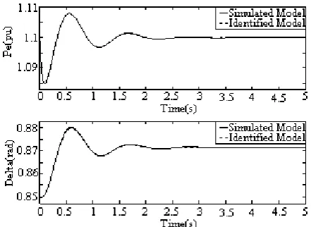
When the field voltage is perturbed with the PRBS, the active output power, the rotor angle and the field voltage are sampled with sample time h=2 millisecond. The operating point is considered to be P=0.9, Q=0.1, vt=0.98. The input/output data collected from the system model in this operating point are shown in Fig. 2.

After simulating the model at operating point P=0.9, Q=0.1 and vt=0.98, the field voltage, the rotor angle and the active power signals are sampled, then matrixes in Eq. (20) and Eq. (25) are obtained. Afterward, θ1 and θ2

are estimated using LSE method. Finally, using the procedure of the previous section, the machine parameters can be calculated. The results of this procedure are given in Table 1.

According to the third column of the Table 1, we can conclude that the estimation error is acceptable. In reality, we don’t know the real value of the parameters. To validate the results, the outputs of real model and the identified one are compared. In the next part, the procedure of model validation is discussed.

4.2 Model Validation

In this section the state space model, achieved in the previous section is validated. For this purpose, several different input signals are applied to the field voltage and the model performance in different operating conditions is observed. The first operating point is considered as P=0.8 pu, Q=0, vt=1.05 pu. The system is excited by a PRBS input and the power and the rotor angle are measured. The results are presented in Fig. 3.

To calculate the estimation error, we use the following indexes [20]:

2 1

1

ˆ ( ( ) ( )) N

k

I y k y k

N =

=

∑

− (43)

Fig. 2 data col

Fig. 3 data col

Table 1 Synch

Parameter

J D

d

x

q

x

d

x

′

′

T

_pdo

(

N FPE

N N

+ =

ˆ ( )(

% R_ee y y P = R − where, n is th number of function. In autocorrelati data remain procedure ac

The auto in Fig. 3 are

llected at opera

llected at opera

hronous Machin

rs Real Val

0.0252 0.500

2.072

1.559

0.568

0.131

1 ( ( ) )

N k

n

y k

n =

+ −

∑

ˆ ( )

2 in y y

N

−

⎛₋ ⎜ ⎝

he number of samples an n the

ee

R

P

on function o in the range ccuracy is call correlation fu given in Fig.

ting point P=0.

ting point P=0.

ne Parameters.

lues Estima Value

2 0.025 0 0.50

2 2.113

9 1.558

8 0.592

0.130

2 ˆ

)−y k( )) 2

, N

⎞ ⎟ ⎠

estimated par d R is the

index, we of error. If m

e 2 2

,

N N

⎛₋ ⎞

⎜

⎝ ⎠

ed satisfactory unctions for th

4.

9, Q=0.1, vt=0.

8, Q=0, vt=1.05

ated es

Error [%]

52 0 7 1.400

32 1.988

89 0.006

2 4.22

04 0.06

(

( rameters, N is

autocorrelat e calculate more than 95%

⎞ ⎟ ⎠

, the estimat y.

he collected d

98.

5.

(44)

(45) the tion the % of tion

data

Fig

wo

R I FP P

δ

cap stu ide vt= in t aut are

wo

I_δ FP

P_R

app som to use tria fie Th res one in p exc ope Co and sys

g. 4 autocorrelat

The values o ould be:

R

1.8521e-00 1.8576

_ 100%

ee

PEδ

δ =

= =

In order to pability in co udies were c entified model =1.02 pu, whe the generator tocorrelation f e given in Fig. The value o ould be:

=2.4416e-00

PE_δ= 2.4637

ee

_δ=100%, As mentione ply the PRBS me papers [14

the input of r e this kind of angular signal ld voltage. T he identificati sults are prese The estimatio e can conclud practice.

In order to cited by the erating poin omparison of t d the system a stem is excited

tion function of

of I, FPE and

R

05, 4.10

e-005,

%, _

P

ee

I FPE

P P

=

o investigate vering the sy carried out. l and the syste en the system field voltage functions for . 6.

ofI_, FPE an 06, I_P =4.1 7e-006, FPE

P_R

ee

_P=10 ed in the beg to the input o 4, 21], it is sh real power pl f signal. In an l, which is th The collected ion procedure

nted in Table on error in the de that the tria perform fur pulse input nt P=1.2 pu the performan at P=1.2 pu, Q d by a pulse si

f Fig. 3.

R ee

P FPE fo

009e-006 4.1132e-100% P

E = =

the propos ystem non-line

The perform em at P=1.1 p is excited by is compared i the collected

nd PR_eefor th

764e-006

E_P =4.2142e-0 00%

ginning of thi of the system. hown that PRB lants, it is not

other example he integral of

data are show e is done ag

2.

e Table 2 is sa angular signa rther, the fiel

with period u, Q=0.15 nce of the ide Q=0.15 pu, vt=

ignal is shown

or PRBS input

006 (46)

sed approach earities, more mance of the pu, Q=0.2 pu, y a step signal in Fig. 5. The data in Fig. 5

he step input

006 (47)

s section, we . Although, in BS is applied t necessary to e, we apply a PRBS, to the wn in Fig. 7. gain and the atisfactory, so al can be used ld voltage is T=4 sec. at pu, vt=0.9. entified model =0.9 when the

n in Fig. 8. t

)

h e e , l e 5

t

)

e n d o a e . e o d s t . l e

130 Iranian Journal of Electrical & Electronic Engineering, Vol. 10, No. 2, June 2014

Fig. 5 data collected at operating point P=1.1, Q=0.2, vt=1.02,

when the input is step signal.

Fig. 6 autocorrelation function of Fig. 5.

Fig. 7 data collected at operating point P=1, Q=0.4, vt=0.95,

when the input signal is triangular.

The value of I and FPE for pulse input would be:

_ 9.2595e-007, _ 1.6253e-007

_ 9.2817e-007, _ 1.6292e-007

I I P

FPE FPE P

δ δ

= =

= = (48)

Since in most real cases the measurements are noisy, in the next Section the effect of noise is studied.

Fig. 8 data collected at operating point P=1.2, Q=0.15, vt=0.9,

when the input signal is a pulse signal.

4.3 Noise Effect

In this part, the effect of white noise on the proposed approach is examined by adding the white noise with different SNR (Signal to Noise Ratio) to the measured outputs. The estimation procedure is done for noisy measurements and the results are presented in Table 3.

According to Table 3, we conclude that for SNR more than 110 the estimated parameters are close to the real values, but for less than it, the estimation error is increased especially for parameters D and J. In addition, we see that the value of xq is robust with respect to the

noise.

Table 2 Synchronous machine parameters when the input signal is triangular.

Parameters Real Values Estimated Values

Error [%]

J 0.0252 0.0252 0

D 0.500 0.511 2.2

d

x

2.072 2.0117 2.91

q

x

1.559 1.5592 0.0012

d

x

′

0.568 0.5544 2.39

′

T

_pdo 0.131 0.1344 2.59

Table 3 estimated parameters for noisy measurements with different SNR.

SNR

Parameters 500 150 120 100 90

D 0.0511 0.0511 0.0523 0.134 0.26

J 0.0252 0.0252 0.0250 0.0174 0.0048

q

x

1.5588 1.5588 1.5588 1.5588 1.5588

d

x

′

0.6068 0.6068 0.6068 0.6091 0.631

d

x

2.1164 2.116 2.116 2.1207 2.1575

d o

T′ 0.1299 0.1299 0.1299 0.1283 0.115

5 Conclusion

In this paper, the theoretical relationbased approach, which uses the known least square error method, has been presented to identify the nonlinear 3rd order synchronous generator state space model parameters. The most important point about the method is to use the linear least square error method to estimate the nonlinear model. In this paper, the field voltage is considered as the machine’s input and the rotor angle and active powers are as the outputs of the machine. Simulation results show that the proposed method has good accuracy for estimation of state space synchronous generator parameters.

Appendix

The main variables of the model in Eq. (1) are: ,

J D: rotor inertia and damping factor

do

T

′

: direct-axis transient time constant

d

x

: direct axis reactance

d

x

′

: direct axis transient reactance q

x : quadrature axis reactance

δ

: rotor angle with respect to the machine terminals

ω

: rotor speed

m

T

: input mechanical torque

e

T

: output electric torque

FD

E

: The equivalent EMF in the excitation coil q

e′: transient internal voltage of armature ,

P Q: terminal active and reactive power per phase

t

v

: generator terminal voltage VB: Infinite bus voltage

, d q

i i : direct and quadrature axis stator currents

References

[1] M. Karrari M and O. P. Malik, “Identification of Heffron-Phillips model parameters for synchronous generators using online measurements”, IEE Proceedings-Generation, Transmission and Distribution, Vol. 151, No. 3, pp. 313-320, 2004.

[2] A. Damaki Aliabad, M. Mirsalim and M. Fazli Aghdaei, “A Simple Analytic Method to Model and Detect Non-Uniform Air-Gaps in synchronous generators”, Iranian Journal of Electrical and Electronic Engineering, Vol. 6, No. 1, pp. 29-35, 2010.

[3] M. Shahnazari and A. Vahedi, “Accurate Average Value Modeling of Synchronous Machine-Rectifier System Considering Stator Resistance”, Iranian Journal of Electrical and Electronic Engineering, Vol. 5, No. 4, pp. 253-260, 2009. [4] M. Kalantar and M. Sedighizadeh, “Reduced

order model for doubly output induction generator in wind park using integral manifold

theory”, Iranian Journal of Electrical and Electronic Engineering. Vol. 1, No. 1, pp. 41-48, 2005.

[5] S. H. Wright, “Determination of Synchronous Machine Constants by Test”, AIEE Transactions, Vol. 50, pp. 1331-1351, 1931.

[6] IEEE Standard 1110-2002, IEEE Guide for Synchronous Generator Modeling Practices and Applications in Power System Stability Analysis, pp. 1-72, 2003.

[7] H. B. Karayaka, A. Keyhani, G. T. Heydt, B. L. Agraval and D. A. Selin, “Synchronous Generator Model Identification and Parameter Estimation From Operating Data”, IEEE Transactions on Energy Conversion, Vol. 18, No. 1, pp. 121-126, 2003.

[8] M. Hasni, O. Touhami, R. Ibtiouen, M. Fadel and S. Caux, “Estimation of synchronous machine parameters by standstill tests”, Mathematics and Computers in Simulation, Vol. 81, No. 2, pp. 277-289, 2010.

[9] E. Mouni, S. Tnani and G. Champenois, “Synchronous Machine Modelling and Parameters Estimation Using Least Squares Method”, Simulation Modelling Practice and Theory, Vol. 16, pp. 678-689, 2008.

[10] M. Dehghani and M. Karrari, “Nonlinear robust modeling of synchronous generators”, Iranian Journal of Science and Technology, Trans. B, Engineering, Vol. 31 (B6), pp. 629-640, 2007. [11] M. Dehghani, M. Karrari, W. Rosehart and O. P.

Malik, “Synchronous Machine Model Parameters Estimation by A Time-Domain Identification Method”, International Journal of Electrical Power and Energy Systems, Vol. 32, No. 5, pp. 524-529, 2010.

[12] V. Vakil , M. Karrari, W. Rosehart and O. P. Malik, “Synchronous Generator Model Identification Using Adaptive Pursuit Method”, IEE proc. Generation, Transmission and Distribution, Vol. 153, No. 2, pp. 247-252, 2006. [13] IEEE Standard 115-1995 IEEE Guide: Test

Procedures for synchronous machines, Part I-acceptance and performance testing Part II-test procedures and parameter determination for dynamic analysis.

[14] M. Karrari and O. P. Malik, “Identification of Physical Parameters of a Synchronous Generator from On-line Measurements”, IEEE Trans. on Energy Conversion, Vol. 19, No. 2, pp. 407-415, 2004.

[15] M. Dehghani and S. K. Y. Nikravesh, “Nonlinear state space model identification of synchronous generators”, Electric Power Systems Research, Vol. 78, No. 5, pp. 926-940, 2008.

[16] Y. Yu, Electric Power System Dynamics, Academic Press, 1983.

132 [17] P. Kun

McGra [18] M. De Space Scale System [19] M. M Metho Evolut Iranian Engine [20] J. P. N

Acade [21] M. R

identif field t Vol. 1

optimization a

ndur, Power aw-Hill Inc., 1 ehghani and Model Param Power Syste ms, Vol. 23, N Mosavi, A. ods in Po tionary Algor n Journal of eering, Vol. 9

Norton, An I emic Press, 19 Rasouli and fication of a b ests”, IEEE T 9, No. 4, pp. 7

Zahra

degree Engine respect the P Concor Canada control and their applica

Ir System Stabil 1994.

S. K. Y. N meter Identifi ms”, IEEE T o. 3, pp. 1449 Akhyani, “P ower System

rithms and G of Electrical 9, No. 2, pp. 76 Introduction

86.

d M. Karra brushless excit Trans. on Ene 733–740, 2004

Gallehdari r and M.Sc. de eering in 2

tively. She is Ph.D. degree

rdia Univer a. Her resear l, system

ations in power

ranian Journa lity and Cont Nikravesh, “S ication in Lar Trans. on Pow 9-1457, 2008. PMU Placem

ms based GPS Receive

and Electro 6-87, 2013. to identificati ari, “Nonlin tation system ergy Conversi

4.

received the B egree in Electr 2005 and 2 currently pursu

in Control rsity, Montr

rch interests identificat r systems.

al of Electrica trol,

tate

rge-wer ment on er”,. onic ion, near via ion,

B.Sc. rical 2009 uing at real, are tion,

uni dyn and

in Un dyn sys

l & Electronic

iversity, Shira namics and con d phasor measu

the Electrica niversity of Te

namical and b stem optimizatio

c Engineering

Maryam D

and M.S engineering Shiraz, Ir respectivel Amirkabir Tehran, Ira assistant pr and com az, Iran. Her ntrol of power s

rement units.

Seyyed Nikravesh

electrical e University Polytechnic the M.Sc. University Columbia respectively al Engineering

echnology. Hi biomedical mod

on.

g, Vol. 10, No.

Dehghani rece Sc. degrees

g from Shira ran, in 1999 ly and her

University o an in 2008. She rofessor in scho mputer engine

research int systems, system

Kamaleddin

received the B engineering fr

of Techno c), Tehran, Iran

and Ph.D. deg of Missouri in 1971 y. Currently, he g Department s research int deling, system

2, June 2014

eived her B.Sc. in electrical az University, 9 and 2002, Ph.D. from f Technology, e is currently an ool of electrical ering, Shiraz terests include m identification

n Yadavar

B.Sc. degree in om Amirkabir logy (Tehran n, in 1966 and grees from the at Rolla and and 1973, e is a Professor at Amirkabir terests include m stability, and

4

. l , , m , n l z e n

r

n r n d e d , r r e d