A Unified Velocity Field for Analysis of Flat Rolling Process

AUT J. Mech. Eng., 1(2) (2017) 139-148 DOI: 10.22060/mej.2017.12585.5374

A Unified Velocity Field for the Analysis of Flat Rolling Process

Mechanical Engineering Department, Razi University, Kermanshah, Iran

ABSTRACT: The subject of this paper is analysis of the flat rolling process by upper bound method. In this analysis the arc of contact has been replaced by a chord and the inlet and outlet shear boundaries of the deformation zone have been assumed as arbitrarily exponential curves. A unified kinematically admissible velocity field has been proposed that permits the possible formation of internal defects. By minimizing the required total power with respect to the neutral point position and the shape of the inlet and outlet shear boundaries, the rolling torque has been determined. The velocity components obtained from the upper bound method have been compared with the FE simulation. The analytical results have been showed a good agreement between the upper bound data and the FE results. A criterion has been presented to predict the occurrence of the split ends and central bursts defects during flat rolling process. Comparison of analytically developed approach for rolling torque and internal defects with published theoretical and experimental data have been showed a good agreement. Finally, the effects of process parameters on the safe and unsafe zones sizes have been investigated. It is shown that with increasing of the friction factor, the safe zone size is decreased.

Review History:

Received: 19 February 2017 Revised: 13 May 2017 Accepted: 2 July 2017

Available Online: 1 October 2017

Keywords: Velocity field Flat rolling Central bursts Split ends 1- Introduction

Flat rolling is the process of reducing the thickness of a long sheet by torques applied through a set of rolls. Internal defects such as central bursts and split ends are the common defects in this process. The investigations on flat rolling have been conducted for decades and various aspects of these processes have been studied. Dyja and Pietrzyk [1] analyzed asymmetric dual hot-rolled sheet using minimum energy and replaced the arc of contact by a chord. Avitzur et al. [2] modeled flat rolling process by using upper bound analysis for rigid perfectly plastic materials that could predict the internal defects by assuming rigid body rotational velocity field for the deformation region. Takuda et al. [3] analyzed the strip rolling process by assuming a simple velocity field with no velocity discontinuities by considering the free deformation zones in front and behind of the roll gap. Turczyn and Pietrzyk [4] analyzed the effect of deformation zone geometry on the internal defects in the flat rolling process by the upper bound method. Prakash and Dixit [5] proposed a model for the steady-state plane strain cold rolling of a strain-hardening material which could predict the roll force and torque with reasonable engineering accuracy over the usual range of process variables. Turczyn [6] analyzed the effect of deformation zone geometry on the internal defects in the rolling process using the upper bound method. He assumed a rigid body rotational velocity field for the deformation region and considered separate velocity fields for each defect and sound flow. Martins and Barata [7] presented an approach to analyze plane strain rolling. They used the upper bound method to estimate the rolling torque and to model the material flow within the region of deformation between the rolls. Dogruoglu [8] introduced a systematic method for constructing kinematically admissible

criterion, as well as the co-line vector inner product method, are used, respectively in the integration of the internal plastic deformation and friction power terms. Jie et al. [19] presented a novel analytical approach predicting roll force in tandem cold rolling is proposed based on elastic and plastic mechanics. A hyperbolic sine velocity field is firstly proposed to get the required minimum roll force in plastic deformation zone in this paper. Shailendra et al. [20] analysed the damage in the hot rolling process using FEM considering different geometric parameters like stock thickness, the percentage of reduction and roll diameter.

In this paper, a unified velocity field for the analysis of flat rolling process and prediction of central bursts and split ends using upper bound method are considered. Based on the observations of the simulation results of the flat rolling process in different conditions with ABAQUS software, a deformation model is proposed. The arc of the contact between the roll and the sheet is replaced by a chord and a unified velocity field including the radial and peripheral velocity components is developed. By minimizing the total power with respect to the neutral point position and the shape of the inlet and outlet shear boundary, the rolling torque and the occurrence of the central bursts and split ends are investigated. The effect of the friction factor and reduction in area on the rolling torque and the safe and unsafe domains are investigated.

2- Upper Bound Analysis

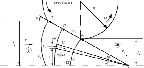
Flat rolling process parameters in a schematic diagram are shown in Fig. 1. Because of the symmetry of the process, only half of the section is considered. The important subject in the upper bound analysis is assuming shear boundaries and the kinematically admissible velocity field that satisfies volume constancy in deformation zone and boundary conditions. In order to determine the velocity field, the arc of contact is replaced by a chord. The material starts as a sheet of thickness 2t_i and is deformed into a sheet of thickness 2t_f , v_i is the initial velocity of the sheet and v_f is the velocity of the product. α is the angle of the line connecting the initial point to the final point of the contact arc with an axis of symmetry. R is the radius and ω is angular velocity of the roll.

2- 1- Geometric description of the deformation zone

Material under deformation is divided into three zones, as shown in Fig. 1. In zones I and III, the material moves rigidly with the velocity v_i and v_f , respectively. The deformation zone (zone II) is surrounded by two shear surfaces S₁ and S₂ and contact surface S₃. The shear boundaries s₁ and s₂ is assumed

to be an arbitrarily curved surface. Using this description, mathematical equations of the shear boundaries s₁ and s₂ are defined in the polar coordinates by

( )

( , ) exp[bi ]

ri i i

θ α θ ρ ρ

α

−

= (1)

( )

( , ) exp[bf ]

rf f f

θ α

θ ρ ρ

α

−

= (2)

and the equation in the deformation zone is

( )

( , ) exp[ ]

( )

exp[ ] ( , ) ( , )

bi f

r

i f

bf i _{g g}

i f

i f

θ α ρ ρ

θ ρ ρ

α ρ ρ

θ α ρ ρ

ρ θ ρ θ ρ

α ρ ρ

− −

=

−

− −

= −

(3)

where ρ_i and ρ_f are shown in Fig. 1, b_i and b_f are the shape factor of the shear boundaries at the inlet and outlet of the deformation zone II, respectively and ρ is the radial position on the contact surface and

( )

( , ) exp[bi f ] gi

i f

θ α ρ ρ θ ρ

α ρ ρ

− −

=

− (4)

( )

( , ) exp[bf i ] gf

i f

θ α ρ ρ

θ ρ

α ρ ρ

− −

=

− (5)

b_i and b_f determine the shapes of the shear boundaries, they can be zero, negative or positive value according to Fig. 2. When they are negative, the shear boundaries move away from the origin O, when they are positive, the shear boundaries move towards the apex O, when they are zero, the inlet and outlet shear boundaries are as cylindrical surfaces.

2- 2- Kinematically admissible velocity field

In zone I and III, material moves as a rigid body in the axial direction. In zone III, velocity from the volume flow balance is

i v_f v_i

f

ρ ρ

= ₍₆₎

By regarding the equilibrium of volume flow, admissible velocity field in deformation zone II can be obtained as

( ) ( )

v dy_x = −U rd_r θ ₍₇₎

Fig. 1. Geometry of the sheet, roll, deformation zone and the shear boundaries.

Thus radial velocity component is v dy_x

U r = − _{r dθ (8)}

where sin i x i v v y r ρ ρ θ = = (9) Then i

r i dy

U v rd ρ ρ θ = −  ₍₁₀₎ where

1 _{sin cos sin cos}

dy dr _r dr

rdθ r dθ θ θ rdθ θ θ

   

= _ + _{ }= + _

    (11)

and

1 i 1 f

i f

g g

dr

rdθ g θ g θ

∂ ∂

= +

∂ ∂ (12)

therefore

1 1

[cos ( )sin ]

i i f

r i i f g g U v g g ρ _{θ θ} ρ θ θ ∂ ∂ = − + + ∂ ∂  ₍₁₃₎

Volume constancy in polar coordinates system is defined as 0

rr zz

ε +ε_θθ+ε = ₍₁₄₎

In polar coordinates, strain rates components are defined as

1

1₍ 1 ₎

2

1₍ 1 ₎

2

1 ( )

2 r rr r z zz r r z z r z zr U r U U r r U z

U U U

r r r

U U z r U U z r θ θθ θ θ θ θ θ ε ε θ ε ε θ ε θ ε ∂ = ∂ ∂ = + ∂ ∂ = ∂ ∂ ∂ = + − ∂ ∂ ∂ ∂ = + ∂ ∂ ∂ ∂ = + ∂ ∂                  (15)

According to the assumption of plane strain process, U_z=0, the peripheral velocity component is

( sin ) sin ( )

sin ( )

i i i f i i i f

f f i f

U v g g v g g

r r

v g g

r θ ρ θ ρ θ ρ θ ∂ ∂ = = = ∂ ∂ ∂ ∂  (16) where

(

)

i f i g f g

g g g g

r r r

∂ ∂

∂ _{= +}

∂ ∂ ∂ (17)

and

1 1

1 1

f f f

f i

i f

f i

i i i

f i

i f

f i

g g g

r r _{g g} g g

g g

g g g

r r _{g g} g g

g g ρ ρ ρ ρ ρ ρ ρ ρ ρ ρ ρ ρ ρ ρ ∂ ₌∂ ∂ ₌∂ ∂ ∂ ∂ ∂  ₊ ∂ ₊ ∂   _{∂ ∂}    ∂ ₌∂ ∂ ₌∂ ∂ ∂ ∂ ∂  ₊ ∂ ₊ ∂   _{∂ ∂}    (18)

The velocity components in deformation zone II are given as

1 1

[cos ( )sin ]

sin ( )

0

i i f

r i

i f

i i i f

z

g g

U v

g g

U v g g

r U θ ρ _{θ θ} ρ θ θ ρ θ ∂ ∂ = − + + ∂ ∂ ∂ = ∂ =    (19)

As it is clear from Eq. (19), on the axis of symmetry U_θ=0, and on the contact surface between roll and sheet U_θ=0, hence incompressibility condition is satisfied. Strain rate components in deformation zone are

2 2 2 2 2 2 2 2 2 2 2

1 [(1 ( ))cos

( )

1 1

( )sin ]

1 [(1 ( ))cos

( )

1 1

( )sin ]

1 _{1 {[ ( )}

2

1 _{( )} 1

i

rr i i f

i f

i f i f

i f

i

i i f

i f

i f i f

i f

i

r i i f

i f

f

f i

v g g

g g r

g g g g

g g r

v g g

g g r

g g g g

g g r

v g g

g g r

g g g θθ θ ρ ε ρ θ ρ ρ θ θ θ θ ρ ε ρ θ ρ ρ θ θ θ θ ρ ε ρ ρ θ ∂ = − + ∂ ∂ ∂ ∂ + − ∂ ∂ ∂ ∂ ∂ = − − + ∂ ∂ ∂ ∂ + − ∂ ∂ ∂ ∂ ∂ = + ∂ ∂ ₊ ∂    2 2 2 2 2 1 1

( ) 1]sin

1 1

( )cos }

0

i i f

i f

i f

i f

zz rz z

g g g

g g g g g g θ θ θ θ θ θ θ θ ε ε ε ∂ ₋ ∂ ₋ ∂ ₊ ∂ ∂ ∂ ∂ ∂ + + ∂ ∂ = = =    (20)

2- 3- Internal power of deformation

The internal power in the upper bound analysis for a rigid perfectly Von-Mises material in deformation zone is

1 2 0

2 ₍1 ₎ 2 3

i _V ij ij

W = σ

∫

where

( i f )

i f i f g g

dV rd rdθ ρg g g g ρ ρ d dρ θ

ρ ρ

∂ ∂

= = + +

∂ ∂ (22)

After substitution and simplification, the internal power of region II is given by

.

2 2 0 0 2 3 ( ) i f

i rr r i f

i f

i f

W g g

g g

g g d d

α ρ θ ρ σ _{ε ε ρ} ρ ρ ρ θ ρ ρ = + ∂ ∂ + + ∂ ∂

∫ ∫

2- 4- Shear power losses

Shear power losses at the shear boundary is

1, 2 0 3

S

S S

W =σ

_∫

For the calculation of the power consumption on each surface of velocity discontinuity, the area of discontinuity and amount of the velocity discontinuity must be determined. Therefore

2 1 i i( , ) 1 ( )i bi

dS ρg θ ρ dθ α

= + (25)

2 1

2 1

(1 ) 1 ( ) sin

(1 ( ) )

i i

i i

i

g b

v v _b

r ρ θ α α ∂ ∆ = − +

∂ ₊ (26)

Thus the shear power losses on the shear surface S₁ is obtained as 1 2 0 0 2

[1 ( ) ] ( , )

3

1

1 sin

1 ( )

i

S i i i i

i i

i

b

W v g

g _d r b α σ _{ρ θ ρ} α ρ θ θ α = + ∂ − ∂ +

∫

Also for the shear surface, S₂ the differential area and amount of the velocity discontinuity can be obtained respectively by

2 2 f f( , ) 1 ( )f bf

dS ρ g θ ρ dθ α

= + (28)

2 2

2 1

(1 ) 1 ( ) sin

(1 ( ) )

f f

f f

f

g b

v v _b

r ρ θ α α ∂ ∆ = − +

∂ ₊ (29)

The shear power losses on the shear surface S₂ is obtained as

2

2 0

2 0

[1 ( ) ] 3

1

( , ) 1 sin

1 ( )

f

S f f

f

f f f

f b W v g g d r b α σ _ρ α θ ρ ρ θ θ α = + ∂ − ∂ +

∫

2- 5- Friction power losses

Friction power losses at the interface of the sheet and the roll in and its general relation is

3 0 3 f S m

W = σ

_∫

where

3

dS =dρ ₍₃₂₎

(cos ( )sin )

r

i i f f i

i

i f i f

v U R

b b v R θ α ω ρ _α ρ ρ ρ ρ _{α ω} ρ α ρ ρ α ρ ρ = ∆ = + = − − − + + + − −  (33) after simplification 0 1 3

cos ( )sin

i

f

f i i

i f f i

i f i f i i

W m v A d

b b R

and A v ρ ρ σ _{ρ ρ} ρ ρ ρ ρ ρ ωρ α α α ρ ρ α ρ ρ ρ = − − = + + − − −

∫

In the rolling process, at only one point along the surface of contact between the roll and the sheet, if the surface velocity of the roll equals to the velocity of the sheet, this point is called neutral point. Between the inlet shear surface and the neutral point, the sheet is moving slower than the roll surface and on the exit side of the neutral point, the sheet moves faster than the roll surface. The position of neutral point is where relative velocity is zero, then

(cos ( N f i N)sin ) 0

i i f

i

N i f i f

b b

v ρ α ρ ρ ρ ρ α Rω

ρ α ρ ρ α ρ ρ

− −

+ + − =

− − (35)

where ρ_N is the radial position of a neutral point on the contact surface.

2- 6- Effective flow stress

For a rigid plastic material, the mean flow stress of the material, is given by

0 0 d ε σ ε σ ε

=

∫

The effective strain is

2 2 2

11 22 22 33 11 33

2[( ) ( ) ( ) ]

9

ε = ε −ε + ε −ε + ε −ε (37)

In plane strain state, ε₃₃=0 so ε₁₁=-ε₂₂, therefore thus

2 ln 3 if

t t

ε = ₍₃₈₎

The behavior of the material is considered as ( )n

K

σ = ε (39)

where K is the strength coefficient and n is the strain-hardening exponent.

Inserting Eqs. (38) and (39) into Eq. (36), the mean flow stress of the material is given by

0 2

( ln )

2- 7- Rolling torque

By the upper bound method, the externally supplied power is less than or equal to the sum of the powers described in the previous sections. The total power is

1 2

i S S f

J∗₌W W_{ +  +}W_{ +}W_{ (41)}

The rolling torque is given by J

T

ω

∗

= (42)

where T is the required rolling torque per unit width of the sheet. The rolling torque is a function of b_i , b_f and ρ_N (radial position of the neutral point). Shape factor b_i determines inlet shear boundary shape and shape factor b_f determines outlet shear boundary shape. The minimum value of rolling torque with respect to the three parameters is the required torque for rolling process in the upper bound analysis. Integrals appearing in the above equations do not have an analytical solution and they have been solved by a numerical method with MATLAB software.

3- Internal defects prediction criteria

External torque is the function of several parameters, including roll radius, area reduction, friction factor and shape factor. In the upper bound analysis, the minimum value of external power with respect to the shape factors is the required power for rolling process. According to the geometrical condition, for a value of shape factor, inlet shear boundary intersects outlet shear boundary on the centerline, Fig. 3. In this dissertation, it can be taken that

( 0, ) ( 0, )

i i f f

r θ = ρ =r θ = ρ ₍₄₃₎

Thus

exp[ ] exp[ ]

i bi f bf

ρ − =ρ − ₍₄₄₎

The equation between shape factors can be obtained as

ln ln

cr cr

i i

i f

f f

t b b

t ρ ρ

− = = ₍₄₅₎

Hence, if the shape parameters obtained from the optimization of external power satisfies Eq. (45), the central burst defects initiate.

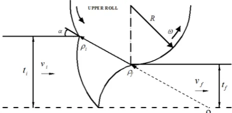
According to the geometrical condition in Fig. 4, if inlet shear boundary intersects outlet shear boundary on centerline and on the line that connects the center of rolls, split ends occurs. That’s mean

tanf

cr t

r = _{α (46)}

After inserting Eq. (46) into Eqs. (1) and (2) and simplification, the critical values are given by

exp( )

tantf_α =ρi −bi (47)

exp( )

tantf_α=ρf −bf (48)

The critical shape factor is tan

cr

i i

f

b Ln t

ρ α

= ₍₄₉₎

and according to Fig. 1,

sini

i t

ρ α

= (50)

after substituting

tan _{( sec )}

sin cr

i i

i

f f

t t

b Ln Ln

t t

α _α

α

= = ₍₅₁₎

(sec )

cr

f

b =Ln α ₍₅₂₎

If the shape factors obtained from the optimization of external power is equal or greater than the Eqs. (51) and (52), the split ends defects are initiated.

4- FE Simulations

The flat rolling process has been analyzed using the proposed approach. In order to obtain numerical boundaries that can be applied to the prediction and prevention of the occurrence of an internal defect in industry, finite element simulations using the proposed approach have been carried out for many combinations of reduction in the area and relative thickness. This means that no internal defect occurs under this combination of process parameters. The FE simulations are conducted on the available commercial explicit/FEM software, ABAQUS, to verify the analytical model and study the effects of upper bound method assumptions on the obtained results. Due to the symmetry of the process, the finite element meshes are generated on the upper half cross section of the sheet. The sheet is meshed by 2D plane strain, linear, four-noded CPE4R elements. The sheet model contains 460 elements. The size of the meshes is 0.0125; because we Fig. 3. Geometric condition to initiate the central burst defect.

used convergence method to obtain the mesh size. In this model, the rolls are modeled as rigid bodies. The rolls are rotated at a constant angular velocity about their axes. For the verification of theoretical study, the results of the rolling torque are extracted from FEM simulations. Fig. 5 shows the FEM mesh model before and after simulation by ABAQUS software.

5- Results and Discussion

In order to verify the validity of the upper bound approach for the flat rolling process, presented in the previous sections, results obtained from the theoretical model are compared with the available experimental data of Ref. [7] and with the finite element simulations results.

The calculation has been carried out under various rolling conditions. The geometric data utilized in the rolling analysis are summarized in Table 1. During theoretical analysis and numerical simulations, m is 0.3 for the contact surface between the roll and sheet, the radius of the rolls is R=148.4 mm, the angular velocity of rolls ω=12 rad/s and the yield stress for aluminum AA5049 80MPa.

The comparisons between the computed results, FEM simulation and the experimental values of Ref. [7] for the rolling torque as a function of the rolling reduction are shown in Fig. 6. It is observed that the proposed velocity field leads to a computationally efficient procedure which makes a good agreement with experimental data. From Fig. 6, it can be seen that the calculated torques are basically in agreement with the measured ones. As expected, the predicted rolling torques are always greater than the experimental and FEM results, because the present theoretical values are upper bound solutions. The reason for such discrepancies may be attributed to the assumption of rigid rolls and difficulties in modeling friction in the contact surface between the rolls and the deforming sheet. It can be checked from Fig. 5 that the rolling torque increases with the increase of reduction in the thickness.

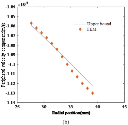
In Fig. 7, the velocity components obtained from the upper bound solution are compared with the FEM simulation results in θ=α/2 in deformation zone. The results show a good agreement between the upper bound data and the FE results. It can be seen that the peripheral velocity components are

very small with respect to the radial velocity components.To compare the numerical results with the experimental results of Ref. [6], the analysis is performed on Aluminum 6061-T6 whose mechanical and physical properties are shown in Table 2. The flow stresses for aluminum at room temperature is σ=410(ε)0.05 _{MPa [6]. The initial thickness t}

i=10 mm, roll radius R=100 mm, angular velocity ω=0.167s-1 _{and friction}

factor m=0.3. Fig. 5. FE meshes, before and after simulation.

Case 2t_o(mm) 2t_f(mm) Reduction (%)

1 6.13 4.91 20

2 6.13 3.94 35

3 6.13 3.02 50

Table 1. Geometric data used for computations [7].

Fig. 6. Comparison of analytical, FEM and Martins experimental data [7] of rolling torque as a function of the

percentage of reduction.

_ _

Young Modulus (GPa) 68.9

Poisson ratio (v) 0.33

Yield stress(MPa) 276

Density (kg/m3_{) 2700}

Strength coefficient (MPa) 410 Strain -hardening exponent 0.05 Table 2. Mechanical properties of Aluminum 6061-T6 [6].

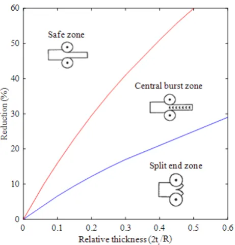
Fig. 8 shows the conditions of area reduction and relative thickness to prevent central burst defects for Aluminum 6061-T6 for the rigid perfectly plastic materials. Also, these results are compared with the experimental data [6]. Fig. 9 shows the conditions of area reduction and relative thickness to prevent split ends defects for Aluminum 6061-T6 for rigid perfectly plastic materials. Meanwhile, these results are compared with the experimental data [6]. The line is a boundary between safe zone and split end zone, in the points that are above the line, we have a rolling process without internal defects, and in points online critical shape factor for the split end occurs. According to the upper bound result, we chose points in the safe zone, split end zone and central burst zone, and simulate them with Abaqus software. Fig. 10a shows the velocity field in the flat rolling process with relative thickness 2t_i /R=0.2, and 40% reduction in the area. The velocity field shows that in this case the internal defects do not occur. In another model, Fig. 10b, the reduction of the area is changed to 20% and the relative thickness is 2t_i /R=0.4 so that it is located in the central burst zone. Also, Fig. 10b shows that, the central burst defects occurred. In another model in Fig. 10c, the reduction of area is changed to 10% and the relative thickness is 2t_i /R=0.5 so that it is located in the split ends zone. Also, Fig. 10c shows that the split ends defects have occurred.

Fig. 11 shows the conditions of area reduction and relative thickness for joint criteria for both defects: central burst and split ends, for Aluminum 6061-T6 for rigid perfectly plastic materials. It can be observed that the range of process parameters where central burst is expected is much wider than that for split ends. The red line is a boundary between safe zone and central burst zone, in the points that are above the red line we have rolling process without internal defects, and in points on red line critical shape factors for central burst occurs and we have a central burst in the process until the blue line, on blue line critical shape factors for split ends occurs and we have split end in the process.

(b)

Fig. 7. Comparison of upper bound and FEM of velocity components (a) Radial and (b) Peripheral velocity components

for 30% reduction in area.

Fig. 8. The comparison of the safe zone and central burst zone predicted by the present model and the Turczyn model [6].

Fig. 9. Comparison of safe zone and split end zone predicted by the present model and the Turczyn model [6].

(a)

Fig. 12 shows the effect of friction factor on the central burst defects initiation situations for Aluminum 6061-T6. It can be seen that by increasing the friction factor, the safe zone size decreased because the value of optimal shape factor decreased. Fig. 13 shows the effect of friction factor on split ends defects initiation situations for Aluminum 6061-T6. It can be seen that with the increase of the friction factor, the safe zone size decreased.

6- Conclusion

In this paper, a prediction of rolling torque and the occurrence of central burst and split ends defects in the flat rolling process by the upper bound method, were presented. A new deformation model and a unified velocity field for the prediction of central bursts defects and the split end is developed. Criteria curves for the safe domains are presented for a wide range of process variables. By using these criteria in rolling practice, it has become possible to predict necessary rolling conditions in order to avoid central burst and split ends defects. The advantages of the presented criterion to other models are the generality of proposed inlet and outlet shear boundaries. This presented criterion predicts both of central burst and split ends defects in simple mathematical equations. (c)

Fig. 10. The deformation zone, (a) for 2t_i /R=0.2 and 40% reduction in area, (b) for 2t_i /R=0.4 and 20% reduction in area,

(c) for 2t_i /R=0.5 and 10% reduction in area.

Fig. 11. Joint criteria for central burst and split ends defects.

Fig. 12. The effect of friction factor on the safe and central burst zone sizes.

References

[1] H. Dyja, M. Pietrzyk, On the theory of the process of hot rolling of bimetal plate and sheet, Journal of mechanical working technology, 8(4) (1983) 309-325.

[2] B. Avitzur, C. Van Tyne, S. Turczyn, The prevention of central bursts during rolling, Journal of Engineering for Industry, 110(2) (1988) 173-178.

[3] H. Takuda, N. Hatta, H. Lippmann, J. Kokado, Upper-bound approach to plane strain strip rolling with free deformation zones, Ingenieur-Archiv, 59(4) (1989) 274-284.

[4] S. Turczyn, M. Pietrzyk, The effect of deformation zone geometry on internal defects arising in plane strain rolling, Journal of Materials Processing Technology, 32(1-2) (1992) 509-518.

[5] R. Prakash, P. Dixit, G. Lal, Steady-state plane-strain cold rolling of a strain-hardening material, Journal of materials processing technology, 52(2-4) (1995) 338-358.

[6] S. Turczyn, The effect of the roll-gap shape factor on internal defects in rolling, Journal of materials processing technology, 60(1-4) (1996) 275-282.

[7] P. Martins, M. Barata Marques, Upper bound analysis of plane strain rolling using a flow function and the weighted residuals method, International journal for numerical methods in engineering, 44(11) (1999) 1671-1683.

[8] A.N. Doğruoğlu, On constructing kinematically

admissible velocity fields in cold sheet rolling, Journal of Materials Processing Technology, 110(3) (2001) 287-299.

[9] S. Ghosh, M. Li, D. Gardiner, A computational and experimental study of cold rolling of aluminum alloys with edge cracking, Journal of manufacturing science and engineering, 126(1) (2004) 74-82.

[10] S.A. Rajak, N.V. Reddy, Prediction of internal defects in plane strain rolling, Journal of materials processing technology, 159(3) (2005) 409-417.

[11] S. Serajzadeh, Y. Mahmoodkhani, A combined upper bound and finite element model for prediction of velocity

and temperature fields during hot rolling process, International Journal of Mechanical Sciences, 50(9) (2008) 1423-1431.

[12] W. Deng, D.-w. Zhao, X.-m. Qin, L.-x. Du, X.-h. Gao, G.-d. Wang, Simulation of central crack closing behavior during ultra-heavy plate rolling, Computational Materials Science, 47(2) (2009) 439-447.

[13] R. Mišičko, T. Kvačkaj, M. Vlado, L. Gulová, M. Lupták, J. Bidulská, Defects simulation of rolling strip,

Materials Engineering, 16(3) (2009) 7-12.

[14] M. Bagheripoor, H. Bisadi, Application of artificial neural networks for the prediction of roll force and roll torque in hot strip rolling process, Applied Mathematical Modelling, 37(7) (2013) 4593-4607.

[15] T.-S. Cao, C. Bobadilla, P. Montmitonnet, P.-O. Bouchard, A comparative study of three ductile damage approaches for fracture prediction in cold forming processes, Journal of Materials Processing Technology, 216 (2015) 385-404.

[16] H. Haghighat, P. Saadati, An upper bound analysis of rolling process of non-bonded sandwich sheets, Transactions of Nonferrous Metals Society of China, 25(5) (2015) 1605-1613.

[17] H. Haghighat, P. Saadati, An upper bound analysis of rolling process of non-bonded sandwich sheets, Transactions of Nonferrous Metals Society of China, 25(5) (2015) 1605-1613.

[18] Y.-M. Liu, G.-S. Ma, D.-W. Zhao, D.-H. Zhang, Analysis of hot strip rolling using exponent velocity field and MY criterion, International Journal of Mechanical Sciences, 98 (2015) 126-131.

[19] J. Sun, Y.-M. Liu, Y.-K. Hu, Q.-L. Wang, D.-H. Zhang, D.-W. Zhao, Application of hyperbolic sine velocity field for the analysis of tandem cold rolling, International Journal of Mechanical Sciences, 108 (2016) 166-173.

[20] S. Dwivedi, R. Rana, A. Rana, S. Rajpurohit, R. Purohit, Investigation of Damage in Small Deformation in Hot Rolling Process Using FEM, Materials Today: Proceedings, 4(2) (2017) 2360-2372.

Pleasecitethisarticleusing:

P. Amjadian and H. Haghighat, A Unified Velocity Field for the Analysis of Flat Rolling Process, AUT J. Mech. Eng., 1(2) (2017) 139-148.