DOI: 10.22075/JRCE.2018.12739.1221
journal homepage: http://civiljournal.semnan.ac.ir/
Extraction of Model Parameters for Reactive Solute
Transport
J. Chabokpour1* and A. Akhoundzadeh2
1. Assistant professor of hydraulic structures, Civil engineering department, University of Maragheh, Maragheh, Iran
2. Head of river engineering department, East Azarbayjan regional water authority Corresponding author:[email protected]
ARTICLE INFO ABSTRACT
Article history:
Received: 12 October 2017
Accepted: 05 February 2018 Rock material is common in the construction of hydraulic structures. In the present study, to the aim is
to examine the reactive solute relationships for transport and degradation processes through the rockfill media. By applying the analytical solution of reactive transport, the 1st to 3rd theoretical temporal moments have been extracted, consequently by applying two methods of curve fitting and temporal moment matching, the coefficients of dispersion and degradation have been exploited. Two rock diameter, two operating discharges and five instantly injection mass have been used as the variables of experiments. The EC sensors with operation software were installed inside the rockfill media and then the experimental breakthrough curves with intervals of 4 seconds have been extracted. It is concluded that both methods are suitable for application of transport and degradation processes inside the media. It was found that by increasing inflow discharges, pore velocity, and media diameters the dispersion coefficient decreases and with a decrease in media diameter or with increase in injection mass the decay rate decreases. The sensitivity analysis on the derived moment equation and also skewness coefficient equation indicated that the velocity and degradation are the most and less effective parameters on the moment equations respectively.
Keywords:
Pollutant Transport,
Reactive Transport Equation, Decay Rate,
Temporal Moments.
1. Introduction
Transport of pollutants through the different type aquatic ecosystems have
transport model of Taylor [1], can been applied. This model is somewhat simple and do not suffer diversity of model parameter and the transport process can be interpreted by only one parameter which is called Dispersion coefficient [1]. The velocity of the mentioned model is cross sectional average velocity. The dispersion coefficient have been computed firstly by routing method which were presented by Fischer [2]. It is believed by previous researchers that after initial mixing of the tracer over the cross section, the Gaussian distribution is dominant and the variance increases linearly by increasing of the time. However, due to the complexity of the dispersion process and geometrical irregularity of the rivers or other flow fields, the explanation of the dispersion process with this model is not accurate [3]. This fact forces the researchers to use other complicated transport models with more model parameters like Transient storage model or aggregated dead zone model [3]. Moreover, different methods exist for extraction of the model parameters. Two applicable and most famous methods are curve fitting and temporal moment methods. Thackston and Schnelle [4] and Fischer et al. [2] tried to catch temporal variation of the concentration in the dead zone and concluded that the dead zone model is applicable for interpretation of the skewness of pollutographs, having long tail in the falling limb. Thackston and
Schnelle [4], Pedersen [5], Nordin and Troutman [6], and Seo and Maxwell [7] confirmed that the transient storage model produce better curve fitting for rebuilding of the long tail of the breakthrough curves. Czernuszenko et al. [8] concluded that there is difficulty in physically interpretation of the dead zone model parameters. Firstly, mathematical closed form of the first to third temporal moments of the dead zone model were extracted by Hays et al. [9] afterwards, the detailed description of them have been investigated by Nordin and Troutman [6] by application of Laplace transform. These relationships have been extracted for instantaneous mass slug over the cross section in the conservative mood for the tracer. After these researchers, the temporal moment relationships for none-conservative mood have been extracted by Schmid [10]. For 1st to 3rd moments and consequently the fourth moment were presented by Seo and Cheong [11].
aggregated dead zone models and Argerich et al. [18] for metabolically active TS model [19].
2. Material and Methods
2.1 Theoretical Approach
If the advection and dispersion of solute is in none-conservative mood like so many solutes such that, the recovered mass from experimental BC1 curves is not
equal with injected mass, it is called reactive solute transport. Putting it differently, in this case, the total mass of contaminants does not recover itself. The one-dimensional mass transport equations by adding degradation term becomes as equation (1).
𝜕𝑐 𝜕𝑡+ 𝑣
𝜕𝑐
𝜕𝑥= 𝐷
𝜕2𝑐
𝜕𝑥2− 𝑘𝑐 (1)
Where 𝐷 is dispersion coefficient and 𝑘 is degradation rate.
Equation (1) is extension of classical AD equation by first-order degradation term and 𝑘 > 0 that implies the contaminant
degrades in its transportation path. By contemplating instantaneous slug release with mass of M to one dimensional flow, analytical solution of equation (1) becomes as equation (2).
𝐶(𝑥, 𝑡) = 𝑀
𝐴√4𝜋𝐷𝑡𝑒𝑥𝑝 (−
(𝑥−𝑉𝑡)2
4𝐷𝑡 − 𝑘𝑡) (2)
Where 𝐴 is cross sectional area, 𝑥 is the location of data acquisition, 𝑉 is the cross
1
) Breakthrough
sectional average flow velocity and 𝑡 is the time matrix [3].
One of the important methods for extraction of dispersion coefficient and degradation rate is curve fitting to the analytical solution (equation 2) with experimental acquired data series.
Since experimental results are normally based on the temporal distribution of concentration (concentration variation versus time at the fixed location), therefore temporal analysis leads to extract characteristics of dispersion and degradation parameters. Applying analytical temporal moments for experimental BC curves, the central tendency of them can be computed. The absolute nth temporal moment of concentration time series 𝐶(𝑡) at the distance of 𝑥 with respect to zero is defined as equation (3):
𝜇𝑛 = ∫ 𝑡𝑛𝐶(𝑡)𝑑𝑡 ∞
0
(3)
And additionally nth normalized temporal moment about zero moment can be defined as equation (4):
𝜇𝑛∗ =𝜇𝑛
𝜇0 =
∫ 𝑡0∞ 𝑛𝐶(𝑥, 𝑡)𝑑𝑡
∫ 𝐶(𝑥, 𝑡)𝑑𝑡0∞ (4)
If the moments is computed with respect to the mean, then nth normalized temporal moment about the mean is 𝑚𝑛
𝑚𝑛 = 1
𝜇0∫ (𝑡 − 𝜇1
∗)𝑛𝐶(𝑡)𝑑𝑡 ∞
0
(5)
𝑚𝑛 = ∑( )𝑛𝑖 𝑛
𝑖=0
𝜇𝑛−𝑖∗ (−𝜇1∗)𝑖 (6)
Where: 𝑖 is an index. The equation (6) is an inverse binomial transform which can be applied to compute normalized central moments of order 1 (mean travel time), 2 (variance) and 3 (skewness)
(Equations of 7, 8 and 9)[20].
𝑚1 = 𝜇1∗ (7)
𝑚2 = 𝜇2∗− (𝜇1∗)2 (8)
𝑚3 = 𝜇3∗− 3𝜇1∗𝜇2∗+ 2(𝜇1∗)3 (9)
By contemplating the equation of (2) as the base equation for our research and also doing some mathematical integrations, the zero ,1st ,2nd and 3rd theoretical temporal moments have been computed respectively as equations of (10), (11), (12) and (13). If the classical advection-dispersion equation was the base function then the zero moment was equal to the 𝑀/𝑄 and due to the constant rate of flow, the mass of the tracer is product of volumetric flow rate and zero moment.
𝜇0 = 𝑀
𝐴√𝑉2 + 4𝑘𝐷
× exp (𝑥𝑉 − 𝑥√𝑉
2+ 4𝑘𝐷
2𝐷 )
(10)
𝜇1 = 𝑀(2𝐷 + 𝑥√𝑉
2+ 4𝑘𝐷)
𝐴(𝑉2+ 4𝑘𝐷)3/2
× exp (𝑥𝑉 − 𝑥√𝑉
2+ 4𝑘𝐷
2𝐷 )
(11)
𝜇2 = 𝑀 [𝑥
2(𝑉2+ 4𝑘𝐷) + 12𝐷2
+6𝐷𝑥√𝑉2+ 4𝑘𝐷 ]
𝐴(𝑉2+ 4𝑘𝐷)52
× exp (𝑥𝑉 − 𝑥√𝑉
2+ 4𝑘𝐷
2𝐷 )
(12)
𝜇3 = 𝑀
[
12𝐷𝑥2(𝑉2+ 4𝑘𝐷)
+120𝐷3
+60𝑥𝐷2√𝑉2+ 4𝑘𝐷
+𝑥3(𝑉2+ 4𝑘𝐷)32 ]
𝐴(𝑉2+ 4𝑘𝐷)72
× exp (𝑥𝑉 − 𝑥√𝑉
2+ 4𝑘𝐷
2𝐷 )
(13)
By manifesting more algebraic operations,
The 0th, 1st, 2nd and 3rd normalized moments with respect to the zero have been computed as equations of (14) to (17). As is illustrated, the normalized zero moment is equal to one.
𝜇0∗ = 1 (14)
𝜇1∗ =(2𝐷 + 𝑥√𝑉
2+ 4𝑘𝐷)
(𝑉2+ 4𝑘𝐷)
(15)
𝜇2∗ =
[𝑥
2(𝑉2+ 4𝑘𝐷) + 12𝐷2
+6𝐷𝑥√𝑉2+ 4𝑘𝐷 ]
(𝑉2+ 4𝑘𝐷)2
𝜇3∗ = [
12𝐷𝑥2(𝑉2+ 4𝑘𝐷) + 120𝐷3
+60𝑥𝐷2√𝑉2+ 4𝑘𝐷 +
𝑥3(𝑉2+ 4𝑘𝐷)32
]
(𝑉2 + 4𝑘𝐷)3
(17)
Furthermore, with regard of equations of (7) to (9) and (14) to (17) by applying some more algebraic operations, the normalized temporal moments with respect to the mean have been computed as the equations of (18) to (21). These relationships can be applied for calculation of mean travel time, temporal variance and skewness coefficient of experimental BC curves.
m1 = μ1∗ =(2D + x√V
2+ 4kD)
(V2+ 4kD)
= tm
(18)
𝑚2 = 𝜇2∗− (𝜇1∗)2
=8𝐷
2+ 2𝐷𝑥√𝑉2+ 4𝑘𝐷
(𝑉2+ 4𝑘𝐷)2 = 𝜎 2
𝑡
(19)
𝑚3 = 𝜇3∗− 3𝜇
1∗𝜇2∗+ 2(𝜇1∗)3
=64𝐷
3+ 12𝐷2𝑥√𝑉2+ 4𝑘𝐷
(𝑉2+ 4𝑘𝐷)3
(20)
𝑆𝐶 = 𝑚3 𝑚2(32)
= 16𝐷 + 3𝑥√𝑉
2+ 4𝑘𝐷
(4𝐷(4𝐷 + 𝑥√𝑉2+ 4𝑘𝐷)3)
(21)
Where: 𝑡𝑚 is mean travel time of the BC curve, 𝜎2
𝑡 is temporal variance of BC
curve and 𝑆𝐶 is skewness coefficient of
BC curve
The first moment has dimension of time and is from t=0 to the center of gravity of
the area under time-concentration curve. Generally, it is called the average travel time of the tracer (equation 22). In many experimental or field conditions, by manifesting more simplification on the second central temporal moment of the classical advection-dispersion equation and neglecting of one ignorable term, the mean residence time of tracer can be approximated as (22):
𝑚1 = 𝜇1∗ = 𝑡𝑚 =
𝑥 𝑉
(22)
Where 𝑡𝑚 is average travel time.
The equation of (23) can be computed from second central moment from classical advection-dispersion equation.
𝐷 = 𝑉
3
2𝑥(𝜇2
∗− (𝜇 1∗)2)
(23)
(𝜇2∗− (𝜇
1∗)2) is variance of BC curve. It
is clear that time temporal variance changes linearly with distance which gives equation (24) [3].
𝐷 = 𝑉 3 2 𝑑𝜎2 𝑡 𝑑𝑥 (24)
On that account, it is apparent that if 𝜎2𝑡
is plotted against 𝑥 as straight line, then the longitudinal dispersivity is a constant value independent to the travel distance and the dispersion coefficient can be calculated applying the slope of straight line from (24).
different moments, one set of two equations (18 to 21) with two unknown parameters can be formed for estimation of dispersion coefficient and degradation rate or by using equation (22) which is operated with large number of previous researchers [19], the dispersion coefficient would be extracted by using one other equation (18 to 21). Hence, the degradation rate would be computed.
2.2 Experimental Data
The experiments have been operated in the rockfill media box with 1.3m length and 0.2m width having erect up and downstream sides. Two rock median diameters of 1.1 and 1.8 cm having porosities of 42 and 47% respectively were imposed inside the media box. Five injection masses of 5, 10, 15, 25 and 50 gr have been introduced instantly at the upstream of media as tracer.
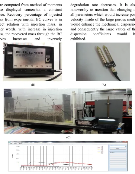
Two completely flowthrough discharges of 0.26 and 0.37 (l/s) have been applied to the media. Pre-calibrated EC sensors were installed at the distances of 0.36 and 1.1m from media entrance, connecting to the data logger with designed software system. Data recording interval was 4 seconds and solution of sodium chloride have been injected instantly at the upstream of the media and simultaneously the data recording has begun. The different parts of the experimental setup has been presented in figure 1.
3. Results and Discussion
were computed from method of moments have displayed somewhat a constant value. Recovery percentage of injected mass from experimental BC curves is in direct relation with injection mass. in other words, with increase in injection mass, the recovered mass through the BC curves increases and inversely
degradation rate decreases. It is also noteworthy to mention that changing of all parameters which would increase pore velocity inside of the large porous media would enhance the mechanical dispersion and consequently the large values of the dispersion coefficients would be exhibited.
(A) (B)
(C)
(D)
Table. 1. Extracted parameters for 1st sensor from curve fitting method to the analytical solution and temporal moments method.
Media diameter (cm) Discharge (l/s) Injection mass (mgr) Recovery *(%) Dispersion coefficient (cm2/s)
CF2 Dispersivity (cm) CF Degradation rate (1/s) CF Dispersion coefficient (cm2/s) MOM3 Dispersivity (cm) MOM Degradation rate (1/s) MOM 1.8 0.26 5000 31.42 8.677 5.903 0.0414 9.0452 5.6540 0.0400 1.8 0.26 10000 45.92 5.523 3.757 0.0283 5.3246 3.8262 0.0357 1.8 0.26 15000 51.80 9.231 6.280 0.0213 7.0506 4.7240 0.0378 1.8 0.26 25000 68.11 5.381 3.660 0.0139 5.1856 3.8254 0.0348 1.8 0.26 50000 93.15 5.213 3.546 0.0033 5.1343 3.7793 0.0349 1.8 0.37 5000 30.81 6.486 3.612 0.0533 8.1416 4.3193 0.0480 1.8 0.37 10000 45.05 6.026 3.355 0.0358 7.0977 4.2527 0.0425 1.8 0.37 15000 47.18 10.266 5.716 0.0307 8.4140 4.8258 0.0441 1.8 0.37 25000 56.66 19.851 11.053 0.0198 12.1302 5.9038 0.0512 1.8 0.37 50000 74.03 10.571 5.886 0.0123 8.9427 5.0197 0.0449 1.1 0.26 5000 30.20 2.933 1.968 0.0510 5.5993 4.2459 0.0336 1.1 0.26 10000 43.45 6.124 4.110 0.0308 5.7696 4.1893 0.0351 1.1 0.26 15000 51.06 5.875 3.943 0.0251 5.0205 3.8412 0.0335 1.1 0.26 25000 69.63 5.398 3.623 0.0137 5.2043 3.9860 0.0334 1.1 0.26 50000 92.42 4.430 2.973 0.0039 4.2947 3.6022 0.0307 1.1 0.37 5000 44.20 3.212 2.007 0.0350 3.6364 2.4167 0.0396 1.1 0.37 10000 59.57 6.642 4.151 0.0192 7.0176 4.6978 0.0378 1.1 0.37 15000 61.87 7.260 4.537 0.0176 5.8664 3.9552 0.0380 1.1 0.37 25000 71.72 5.656 3.535 0.0136 4.7959 3.5657 0.0347 1.1 0.37 50000 97.44 5.777 3.611 0.0021 5.6281 4.0493 0.0355
*Recovery percentage is calculated by dividing of the recovered mass by experimental BC curve to the injection mass.
Table. 2. Extracted parameters for 2nd sensor from curve fitting method to the analytical solution and temporal moments method.
Media diameter (cm) Discharge (l/s) Injection mass (mgr) Recovery (%) Dispersion coefficient (cm2/s)
CF Dispersivity (cm) CF Degradation rate (1/s) CF Dispersion coefficient (cm2/s)
MOM Dispersivity (cm) MOM Degradation rate (1/s) MOM 1.8 0.26 5000 34.46 18.696 7.922 0.0215 24.2937 9.6010 0.0215 1.8 0.26 10000 43.38 10.565 4.477 0.0166 10.7374 4.3397 0.0217 1.8 0.26 15000 54.95 16.785 7.112 0.0122 36.4640 16.0166 0.0187 1.8 0.26 25000 57.02 11.869 5.029 0.0111 11.3712 4.7388 0.0210 1.8 0.26 50000 73.45 11.857 5.024 0.0062 12.0859 5.0310 0.0210 1.8 0.37 5000 22.08 20.823 7.545 0.0353 25.4458 8.0742 0.0270 1.8 0.37 10000 35.96 16.076 5.825 0.0233 17.0280 5.5472 0.0267 1.8 0.37 15000 42.04 21.033 7.621 0.0192 19.6074 6.2630 0.0271
2
) Curve Fitting
3
1.8 0.37 25000 46.52 32.644 11.828 0.0160 19.6462 5.8572 0.0291 1.8 0.37 50000 60.27 22.631 8.200 0.0110 17.6963 5.7354 0.0268 1.1 0.26 5000 17.53 7.029 3.138 0.0377 14.3434 6.7434 0.0184 1.1 0.26 10000 29.83 10.653 4.756 0.0237 13.7571 5.9007 0.0203 1.1 0.26 15000 35.84 10.303 4.599 0.0200 11.7250 5.1558 0.0199 1.1 0.26 25000 42.05 10.697 4.775 0.0168 11.5724 5.2019 0.0194 1.1 0.26 50000 54.23 8.902 3.974 0.0125 10.9006 5.1183 0.0186 1.1 0.37 5000 21.48 7.645 3.058 0.0353 14.2303 5.5916 0.0222 1.1 0.37 10000 38.90 12.764 5.106 0.0205 24.6519 9.5134 0.0220 1.1 0.37 15000 39.43 12.481 4.992 0.0201 15.2303 5.9076 0.0224 1.1 0.37 25000 43.88 11.285 4.514 0.0184 12.1847 5.0363 0.0211 1.1 0.37 50000 52.10 12.371 4.948 0.0146 13.6492 5.6433 0.0210
The figures of 2(a, b) are indicating some examples of experimental and analytical BC curves which have been conducted at the two above mentioned positions. As is presented, by moving along the large porous media, the dispersion and degradation processes have acted and the downstream curves have indicated a lower magnitude in climax point. In addition to the experimental curves, analytical curves by applying the dispersion and degradation coefficients, which were exploited from both above-mentioned methods, have been depicted. As a conclusion it can be implied that both of the methods is beneficial and can be applied to the tracer tests. Furthermore, the depicted curves indicates asymmetry between two limbs of the BC curves because of transient storage of tracer inside the media and gradually outgoing from that.
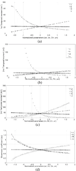
The sensitivity analysis for 1st to 3rd temporal moments and skewness coefficient have been arranged. 4 parameters of velocity, degradation rate,
dispersion coefficient and length scale were chosen as variables of the moments. The real magnitudes for mentioned parameters were selected to examine the sensitivity of them in the moment equations. Since all the parameters are in different dimensions, the normalized form of them have been computed in order to arrange them in the limited domain. The normalization process were accomplished applying equation of (25).
𝑥𝑛 =
(𝑥𝑖− 𝑥̅)
𝑠𝑡𝑑(𝑥𝑖)
(25)
but in skewness coefficient, it operate a reverse none-linear tendency.
(a)
(b)
Fig. 2. Experimental and analytical BC curves for a) injection mass equal to 5000 (mgr), median diameter of media d=1.8 cm and entrance discharge equal to 0.26 (l/s) b) Injection mass equal to 15000 (mgr),
median diameter of media d=1.1 cm and entrance discharge equal to 0.37 (l/s).
-5.00E+01 0.00E+00 5.00E+01 1.00E+02 1.50E+02 2.00E+02 2.50E+02 3.00E+02 3.50E+02
0 20 40 60 80 100 120 140 160 180 200
Concentrati
on
(ppm)
Time (s)
0.36m-Experimental
1.1m-Experimental
0.36m-Temporal Moment
1.1m- Temporal Moment
0.36m-Curve Fitting
1.1m-Curve Fitting
-2.00E+02 0.00E+00 2.00E+02 4.00E+02 6.00E+02 8.00E+02 1.00E+03 1.20E+03 1.40E+03
0 20 40 60 80 100 120 140 160 180 200
C
oncen
trati
on
(ppm)
Time (s)
0.36m-Experimental
1.1m-Experimental
0.36m-Temporal Moment
1.1m-Temporal Moment
0.36m-Curve Fitting
(a)
(b)
(c)
(d)
Fig. 3. Sensitivity analysis for moment equations a) 1st temporal moment versus normalized parameters b) 2nd temporal moment versus normalized parameters c) 3rd temporal moment versus normalized
The decay rate reveals a gentle decreasing manner in the all moment and skewness coefficient equations such that it has the lowest impact on the model equations. The parameter of the dispersion coefficient has very interesting role in which in the 1st and 2nd moment equation it has linear trend but decreasing in the 1st and increasing in the 2nd moment. For 3rd moment equation, the dispersion coefficient shows non-linear increasing manner. Moreover, in the skewness coefficient equation, non-linear increasing manner with respect to the dispersion coefficient has been observed.
4. Summary and Conclusions
Sometimes, the injected mass as tracer in different type flow fields cannot be recovered totally. Consequently, the reactive equations is beneficial for application. In this research, the theoretical temporal moments were derived from direct integration from analytical equation of the advection-dispersion including first-order reactive term. The magnitudes of the decay rate and dispersion coefficients have been extracted for one experimental data series applying two different methods named least square curve fitting and temporal moment. The outcomes reveals proficiency of the both of these methods. Notwithstanding, the rebuilt breakthrough
curves by the coefficients of LSCF shows a better agreement with the experimental BC curves. The results revealed that the magnitudes of the both of the mentioned coefficients illustrated spatial variation along the porous media. All geometrical and hydraulically parameters which enhances mechanical dispersion processes causes enhancing in the both of the coefficients. The sensitivity analysis were demonstrated for the obtained moment equations by changing of the 4 involved parameters. It is concluded that the velocity parameter is the most effective parameter among others which shows a reverse effect in the different order moment equations. Furthermore, the degradation rate is the less effective parameter in the all the moment and skewness coefficient equations which indicate reverse linear decreasing manner.
5. Acknowledgements
The author would like to appreciate from financial support from Research Minister of University of Maragheh, Grant number of 94D369.
REFERENCES
[2] Fisher, H.B., List, E.J., Koh, R.C., Imberger, J. and Brooks, N.H. (1979). “Mixing in Inland and Coastal Waters.” Academic. New York.
[3] Chanson, H. (2004). “Environmental hydraulics of open channel flows.” Frist Edition. Elsevier Butterworth-Heinemann Linacre House. Jordan Hill. Oxford. [4] Thackston, E.L. and Schnelle, K.B.J. (1970).
“Predicting effects of dead zones on stream mixing.” Journal of the Sanitary Engineering Division, 96: 319–331. [5] Pedersen, F. B. (1977). ‘‘Prediction of
longitudinal dispersion in natural streams.’’ Hydrodynamics and Hydr. Engrg. Ser. Paper No. 14, Technical University of Denmark, Lyngby, Denmark. [6] Nordin, C.F. and Troutman, B.M. (1980). “Longitudinal dispersion in rivers: the persistence of skewness in observed data.” Water resources research, 16(1):123–8. [7] Seo, I. W., and Maxwell, W. H. C. (1992).
‘‘Modeling low-flow mixing through pools and riffles.’’ J. Hydr. Engrg., ASCE, 118(10), 1406–1423.
[8] Czernuszenko, W., and Rowinski, P. M. (1997). “Properties of the dead-zone model of longitudinal dispersion in rivers.” Journal of Hydraulic Research, 35(4), 491– 504.
[9] Hays, J. R., Krenkel, P. A., Karl, B., and Schnelle, J. (1966). ‘‘Mass transport mechanisms in open-channel flow.’’ Tech.
Rep. 8, Dept. of
Civ. Engrg., Vanderbilt University, Nashville, Tenn.
[10] Schmid, B. H. (1995). ‘‘On the transient storage equations for longitudinal solute
transport in open channels: Temporal moments accounting for the effects of first-order decay.’’ J. Hydr. Res., Delft, the Netherlands, 33(5), 595–610.
[11] Seo, I.W. and Cheong, T.S. (2001). “Moment-based calculation of parameters for the storage zone model for river dispersion.” Journal of hydraulic engineering, 127(6):453–65.
[12] Harvey, C. F., and S. M. Gorelick (1995). “Temporal moment-generating equations: Modeling transport and mass transfer in heterogeneous aquifers.” Water Resour. Res., 31(8), 1895–1911.
[13] Luo, J., O. A. Cirpka, M. Dentz, and J. Carrera (2008). “Temporal moments for transport with mass transfer described by an arbitrary memory function in heterogeneous media.” Water Resour. Res., 44, W01502.
[14] Schmid, B. H. (2003). “Temporal moments routing in streams and rivers with transient storage.” Advances in Water Resources, 26, 1021–1027.
[15] Goltz, M. N., and P. V. Roberts (1987). “Using the method of moments to analyze three-dimensional diffusion-limited solute transport from temporal and spatial perspectives.“ Water Resour. Res., 23(8), 1575–1585.
[16] Cunningham, J. A., and P. V. Roberts (1998). “Use of temporal moments to investigate the effects of nonuniform grain-size distribution on the transport of sorbing solutes.” Water Resour. Res., 34(6), 1415–1425.
storage and aggregated dead zone models of longitudinal solute transport in streams.” Water Resour. Res., 36(1), 213–224. [18] Argerich, A., R. Haggerty, E. Martı, F.
Sabater, and J. Zarnetske (2011). “Quantification of metabolically active transient storage (MATS) in two reaches with contrasting transient storage and ecosystem respiration.” J. Geophys. Res., 116, G03034.
[19] Majedi Asl, M., Jafari, R. (2012). “The Mathematical Modeling of Self-Purification of the Zarjoob River for Justification of Emission.” Journal of Environmental Science and Engineering, A1:1-10.