The Thirty-Third AAAI Conference on Artificial Intelligence (AAAI-19)
A Distillation Approach to Data Efficient Individual Treatment Effect Estimation
Maggie Makar
CSAIL, MIT Cambridge, MA [email protected]Adith Swaminathan
Microsoft ResearchRedmond, WA [email protected]
Emre Kıcıman
Microsoft Research Redmond, WA [email protected]Abstract
The potential for using machine learning algorithms as a tool for suggesting optimal interventions has fueled significant in-terest in developing methods for estimating heterogeneous or individual treatment effects (ITEs) from observational data. While several methods for estimating ITEs have been re-cently suggested, these methods assume no constraints on the availability of data at the time of deployment or test time. This assumption is unrealistic in settings where data acquisi-tion is a significant part of the analysis pipeline, meaning data about a test case has to be collected in order to predict the ITE. In this work, we present Data Efficient Individual Treat-ment Effect Estimation (DEITEE), a method which exploits the idea that adjusting for confounding, and hence collect-ing information about confounders, is not necessary at test time. DEITEE allows the development of rich models that exploit all variables at train time but identifies a minimal set of variables required to estimate the ITE at test time. Using 77 semi-synthetic datasets with varying data generating pro-cesses, we show that DEITEE achieves significant reductions in the number of variables required at test time with little to no loss in accuracy. Using real data, we demonstrate the utility of our approach in helping soon-to-be mothers make planning and lifestyle decisions that will impact newborn health.
Introduction
When designing a learning system to perform interventions—whether through direct action or indi-rect recommendation—it is important to model the intervention’s causal effect on target outcomes rather than the correlation between the two (Pearl 2009). Establishing a causal relationship between the intervention and the outcome is necessary to ensure that the desired outcome will happen with high probability should the intervention be carried out. While conventional causal inference techniques focus on calculating the average effect of an interven-tion over a populainterven-tion (Rosenbaum and Rubin 1983; Rosenbaum 2002), more recent methods focus on es-timating personalized or individual treatment effects (ITEs; sometimes referred to as conditional average treat-ment effects) from observational data (Johansson, Shalit, and Sontag 2016; Athey, Tibshirani, and Wager 2016;
Copyright c2019, Association for the Advancement of Artificial Intelligence (www.aaai.org). All rights reserved.
Shalit, Johansson, and Sontag 2017; Wager and Athey 2018). These approaches perform what we call ITE dis-covery, i.e., using observational data to discover the causal effect of a treatment for any individual in the population.
To calculate individual treatment effects, these methods assume that all the variables used to train the ITE discov-ery model continue to be available for individuals at test time. Unfortunately, there are often significant practical con-straints limiting the availability of data about new test cases. For example, a physician may need to decide if a treat-ment will benefit a specific patient without having all rel-evant medical test results at her disposal. In this situation, the physician would prefer to identify and conduct the min-imal set of necessary medical tests to accurately estimate the treatment effect for this patient. Similar situations arise with social workers, loan officers, judges and other decision-makers; they might need to identify a small set of attributes for an individual in order to accurately estimate the effect of a decision. We refer to this process asITE prediction.
ITE prediction and ITE discovery are significantly differ-ent tasks. For an algorithm to perform reliable ITE discov-ery, it needs to perform two functions:adjustment for con-founding and estimation of heterogeneous effects. Adjust-ment for confounding accounts for the fact that treatAdjust-ment was not randomly assigned in the observational data, and that people who receive the treatment often have systemati-cally different outcome likelihoods than those who did not. For example, sicker patients who are more likely to die are also more likely to receive aggressive treatments. Hetero-geneous effects estimation accounts for the fact that indi-viduals respond differently to the same treatment based on their characteristics. For example, elderly or frail patients may have a systematically adverse response to an aggres-sive treatment. To adjust for confounding, researchers could appeal to a number of statistical methods that utilize a set of variables,confounders, to make the treated and the con-trol populations appear statistically similar. To perform reli-able ITE prediction, we only need good estimation of hetero-geneous effects (which depend on individual characteristics that are referred to aseffect modifiers).
ef-Treatment effect modified by z = 0
Treatment effect modified by z = 1 Average
treatment effect
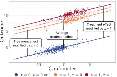
Figure 1: ITE varies by effect modifiers (z), not by the con-founder
fect varying with the value of the effect modifier,z. Thex -axis shows the confounder, while they-axis shows the value of the outcomes. To simplify this didactic example, we as-sume thatzdoes not affect the outcome for the non-treated group, but that is not an assumption that is necessary for our work. Note that, while outcomes vary with the confounder, the treatment effect does not; the ITE is independent of the confounders (since the dashed line and the solid blue line are parallel) but not the effect modifiers. This suggests that while both confounders and effect modifiers are required at training time, only the latter are required at test time. In situ-ations where confounders are high dimensional while effect modifiers are not, requiring the full set of variables at test time would be demanding a number of variables that might be redundant for ITE prediction.
In this work, we exploit the difference between the tasks at training time (ITE discovery) and test time (ITE predic-tion) to reduce the number of variables required at test time. We develop an approach similar in spirit to model compres-sion or knowledge distillation methods. Our Data Efficient Individual Treatment Effect Estimator (DEITEE) proceeds in two steps. At train time, a base model is tasked with both confounding adjustment and estimation of heterogeneous treatment effects. Next, a lightweight decision tree identifies the variables associated with the most variance in ITE and requires only these variables to be queried during test time. In addition to reducing the number of variables required at test time, DEITEE also:
1. Allows “early estimation”: the individual can receive an ITE estimate after each query before answering all queries. 2. Identifies personalized questionsbased on the individ-ual’s collected profile, by dynamically following different pathways in the tree to collect the most informative variables for different individuals.
Testing DEITEE on 77 semi-simulated datasets with vary-ing data generatvary-ing processes, we find that DEITEE achieves large reductions in the number of variables required to com-pute the ITE with little to no loss in accuracy. We find that the variables queried tend to be effect modifiers even though our method provides no guarantees that they would be. Fi-nally, using a dataset of over 89 thousand soon-to-be moms, we show that our method can be used to help them make
de-cisions about their habits and lifestyle choices that are con-sequential to their newborns’ health.
Related Work
Recent work in machine learning and causality has focused on moving away from average treatment effect estimation to personalized, ITE estimation. Approaches to modeling the ITE span a large spectrum of statistical tools including the use of Bayesian non-parametric models, random forests, and deep neural networks (Athey, Tibshirani, and Wager 2016; Athey and Imbens 2016; Johansson, Shalit, and Sontag 2016; Shalit, Johansson, and Sontag 2017; Alaa and van der Schaar 2018; 2017; Hill 2011). These approaches, however, assume that data available at training time will also be read-ily available at test time, not taking into account the fact that data collection might be a non-trivial part of the pipeline at test time. Alaa and van der Schaar discuss the distinc-tion between accounting for confounding, or selecdistinc-tion bias, and ITE estimation. Their analysis focuses on the relative importance of accounting for selection bias versus response surface estimation (and hence ITE heterogeneity estimation) in small and large samples. Previous approaches to ITE es-timation should be viewed as complementary to the work presented here. In fact, we use these algorithms as a part of our suggested approach.
Importantly, existing work in ITE estimation can be clas-sified into two: algorithms that model the treatment effect only (e.g., Athey, Tibshirani and Wager 2016; Athey and Imbens 2015) and those which model counterfactual out-comes (e.g., Hill 2016; Johansson, Shalit and Sontag 2016). The former give an estimate of the difference between the outcome under the intervention and the outcome under non-intervention, while the latter give a full estimate of the out-comes under intervention and non-intervention. Estimating treatment effects only is important in situations where the decisions are made based on the difference between the ben-efit of the treatment and its cost (i.e., return on “investment”) or if the outcome under non-treatment is known (e.g., a pa-tient will most likely die if untreated). Our work falls under the category of treatment effect rather than counterfactual outcome estimation.
and we exploit that difference to create a more compressed model requiring fewer features at test time.
Preliminaries
Without loss of generality, we frame our discussion using the Neyman-Rubin framework of potential outcomes (Rubin 2005). We focus on binary treatmentst∈ {0,1}. We assume that for a single individual, e.g., a patient, with feature vec-torx, there exist two potential outcomesY1andY0but only one of them is observed. We denote the observed outcome by lowercasey. To emphasize that the unobserved or coun-terfactual outcome is a function of the individual features, we useYt(x)to refer to the counterfactual outcome for an individual with featuresxunder treatmentt. The ITE,τ(x), is hence also a function ofxand is equal toY1(x)−Y0(x). We make the classical assumptions of strong ignorability:
Yt
t | x; overlap:0 < p(t = 1|x) < 1∀x; and consis-tency:y=Y0ift= 0andy=Y1ift= 1.In addition, we assume that the the counterfactual out-come can be expressed as:Yt(x) = g(x) +1{t=1}·f(z).
Throughout the text, we refer toz⊆xas effect modifiers. This functional decomposition is not a restrictive assump-tion asgandfcan belong to any complicated function class andzcan include all variables.
We assume that a large dataset D = {xi, ti, yi}Ni=1 is available at training time, but that data for a new test case, xj, must be acquired with some non-trivial cost to compute an ITE estimate for individualj. We assume that all features have an equal cost at test time, but our approach can be extended to incorporate different costs for different features. We distinguish between two tasks
ITE Discovery: The goal is to develop an algorithm that takesDas input, and outputs a functionτˆ : X 7→ R
such thatτˆ(x)≈τ(x)for all individualsx∈X.
ITE Prediction: For a particular individual we ob-serve a subset of variablesz, and we must output a valueˆe
such thatˆe≈R
Pr(x| z)τ(x)dx. ITE Discovery can be a useful sub-goal for this problem, since we might be able to approximateeˆ≈R
Pr(x|z)ˆτ(x)dxusingDandτˆ.
Our goal is data-efficient ITE prediction. That is, what is a sufficient set of variableszwe must observe about an in-dividual, and what should our estimateeˆbe for that person?
Motivating Insights
Consider the example of a physician trying to estimate the effect of conducting an aggressive surgery. She would only choose to do the surgery if it increases her patient’s life expectancy. What demographic questions and medical tests should she ask/run so that she gets an accurate estimate of post-surgery change in life expectancy?
Heterogeneous treatment estimation From the defini-tion of ITE, we have that:
τ(x) =Y1(x)−Y0(x) =g(x) +f(z)−g(x) =f(z).
This reveals thatτis a function ofzrather than all ofx. In scenarios where thezis of a much smaller dimension than x, there is a clear advantage to only collecting the effect modifiers z. Even if all the features are effect modifiers there is an advantage to ordering the variables according to the magnitude of effect modification and only collecting the top modifiers in budget-constrained test scenarios.
Insight 1: We only need to collect effect modifiers for ITE prediction.
Personalized feature selection Consider the case where life expectancy of the patient has the following form:
f(z) =1{zv>c}·exp(zlA) +1{zv≤c}·exp(zlB),
wherezvdenotes vitals,zlA,zlBdenote results of lab test A and B respectively andcis some constant. Note, lab test A is only relevant for patients for whomzv> cwhile lab test B is only relevant for patients for whomzv ≤c. The ideal data collection process mimics that hierarchical dependency structure, collecting the vitals first and then deciding which lab test to conduct next based on their values.
Insight 2: Individuals may have different effect modi-fiers. We can personalize their queries.
Identifying axes of variance Consider the situation where two effect modifiers, say, zv, andzlA, are functions of another variablex. In that case, queryingx, even though it might not be an effect modifier, is more efficient than querying zv, and zlA for patients with zv > c. It might be that for some applications, it is important to medically understand the factors that affect the treatment effect but for the purposes of efficient data collection, which is our main aim, identifying the variables associated with the most variance in the ITE is sufficient.
Insight 3: Collecting variables that induce the highest variance is sufficient for ITE prediction.
Direct regularization for ITE discovery does not work One might wonder whether some form of variable regu-larization can be applied during ITE discovery to ensure feature sparsity and enable data-efficient ITE prediction as a side-effect. If the regularization penalty leads to excluding confounders inx\z(that affect both treatment likelihood and the outcome), our estimates will be unnecessarily biased. If it leads to excluding any of the variables in z, it would be ignoring an axis of heterogeneity, essentially lumping together groups with diverse ITEs.
Method: A Distillation Approach
assumptions later. Our objective function is defined as:
I∗, θ∗= arg min
I,θ 1 N X i
τi−fθ xIi 2
s.t.|I| ≤K, (1)
whereI denotes an index set,xI denotes the subset of the vector x formed by picking the dimensions, d ∈ I and
θ parametrizes the mapping from xI to τ. This is essen-tially an L0 regularization problem which is computationally intractable, since it requires optimization over the discrete space of all possible index sets.
Because L0 regularization is intractable, we tackle the problem iteratively, only seeking to find one relevant feature at a time. We opt for an iterative approach because it can be stopped at any point, giving us an early estimate of the ITE based on the variables selected so far. In the first iteration we find the feature associated with the most variance in the entire population, which entails solving:
d∗1, θ∗1= arg min
d,θ 1 N X i
τi−fθ xdi
2
whereddenotes a dimension ofxandd∗
k denotes the opti-mal dimension picked in thekthiteration. For thekth itera-tion, the objective is defined as:
d∗k, θk∗= arg min d6∈{d∗1:k−1},θ
1 N X i
τi−fθ x
(d∗1:k−1,d)
i
2
,
and so forth. While this iterative approach has the advantage of allowing early estimation, it makes the assumption that there is a single set of variables that is relevant for the entire population. To relax that assumption, we redefine the opti-mization function such that at each iteration it picks the di-mension associated with the highest variation and splits the population into two distinct, less heterogeneous subgroups for which we can repeat the process recursively, optimizing this objective for each group separately.
To do so, we introduce a splitting function,hφ(x)which gives a partition π, splitting the population into subgroups
`1and`2. For simplicity, we consider binary splits. Our ob-jective function for the first iteration can now be re-written:
d∗1, θ ∗ 1, φ
∗
1= arg min
d,θ,φ 1 N X i
τi−fθ xdi;hφ(xdi) 2
Importantly, since our objective is to minimize data collec-tion, we require that the same variable that is used for es-timation is also used for splitting:fθ andhφ both depend on the samexd
i. The objective function for thekthiteration can now be defined separately for each of the`j partitions created in iterationk−1:
d∗k,j, θk,j∗ , φ∗k,j = arg min
d,θ,φ
1
#(i:i∈`j)
X
i
τi−fθ x
(d∗1:k−1,d)
i ;hφ(x
(d∗1:k−1,d)
i )
2
where#(i: i∈`j)denotes the number of samples falling in subgroupjof partition induced byhφ(x
(d∗
1:k−1,d)
i ). Note
that when hφ is a simple thresholding function and fθ is the mean of the sub-population satisfying the threshold, this objective function is identical to the objective function of a simple decision tree:
Π∗,µ∗=X j
arg min
Π,µ
1 #(i:i∈`j)
X
i
τi−µj(`j)
2
(2)
whereµj(`j)is the mean of leafj,µ={µj}for alljandΠ is a partition, withΠ ={`j}Mj , whereMis the total number of leaves in the tree.
The tree can be grown until a pre-specified number of queries K is achieved or until further queries do not lead to further improvements in the accuracy, meaning:
1 #(i:i∈`j)
X
i
τi−µj(`j)
2
< (3)
for some smallfor all possible partitions.
Of course, we never have access toτi. Instead, we assume that at training time, we have access to an algorithm A :
D → τ˜(x). Meaning an algorithm that learns a functional mapping from the full set of features to the ITE. Using this algorithm, we can train a model to compute an approximate estimate ofτi for alliin the training data. We refer to this model as the base model and denote this approximation with
e
τi. Replacingτiwithτei, the objective function in 2 can now
be rewritten as:
Π∗,µ∗=X
j
argmin
1
#(i:i∈`j)
X
i
e
τi−µj(`j)
2
At test time, we need to only query the variables that define the partition in the order defined by the partition hier-archy. The depth of the partitionKcan either be defineda priorior the partition trees can be allowed to grow until the reduction in variance is less than a tolerance parameter. Al-ternativelyorKcan be acquired through cross-validation against the base model’s estimates ofτfor the validation set.
Why trees? The regularization problem expressed in equation 1 could have been approximated in a number of ways. We chose decision trees for several reasons. First, the tree could be fully trained at training time, but traversed up to some depth K < the maximum depth at test time en-abling the end user to stop whenever their budget of queries is exhausted. In addition, different pathways are defined by different variables, which encodes our intuition that different features will be relevant for different individuals. Finally, decision trees are easy to train and interpret, which adds little to no overhead to the inherently complicated ITE estimation process making this approach user-friendly.
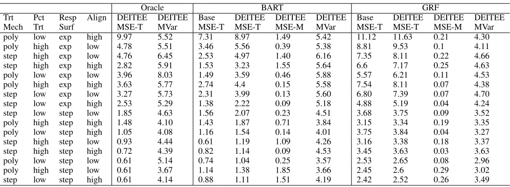
Table 1: DEITEE leads to large reductions in required features at test time with little to no loss in accuracy
Oracle BART GRF
Trt Pct Resp Align DEITEE DEITEE Base DEITEE DEITEE DEITEE Base DEITEE DEITEE DEITEE Mech Trt Surf MSE-T MVar MSE-T MSE-T MSE-M MVar MSE-T MSE-T MSE-M MVar poly low exp high 9.97 5.52 7.31 8.97 1.49 5.42 11.12 11.63 0.21 4.30 poly high exp low 4.78 5.51 3.46 5.56 0.39 5.38 8.81 9.53 0.1 4.11 step high exp low 4.76 6.45 2.53 4.97 1.40 6.16 7.35 8.11 0.22 4.66 step high exp high 2.82 5.91 1.53 3.23 1.55 5.64 6.6 7.17 0.25 4.63 poly low exp low 3.96 8.03 1.49 3.59 0.46 5.88 5.57 6.21 0.11 4.53 poly high exp high 3.63 5.77 2.74 4.4 0.15 5.58 7.54 8.11 0.07 4.38 step low exp low 3.27 5.73 2.31 3.99 0.13 5.60 6.80 7.39 0.07 4.70 step low exp high 2.53 5.29 1.38 2.22 0.09 5.18 4.88 5.19 0.04 4.24 step low step low 1.85 4.63 1.56 2.07 0.23 4.51 3.68 3.75 0.09 3.52 poly high step high 1.48 4.10 1.43 1.87 0.71 3.84 3.15 3.34 0.19 3.35 poly low step high 1.05 4.08 1.16 1.54 0.14 4.01 3.75 3.84 0.04 3.27 step high step low 0.93 4.44 0.61 1.19 1.09 4.26 3.16 3.38 0.18 3.37 step high step high 0.72 4.39 0.82 1.14 0.09 4.53 3.45 3.63 0.03 3.63 poly low step low 0.61 5.14 0.74 1.04 0.25 3.57 2.53 2.65 0.08 2.96 poly high step low 0.61 3.67 1.14 1.38 1.85 3.66 2.45 2.6 0.29 3.02 step low step high 0.61 4.14 0.88 1.11 1.51 4.19 2.42 2.52 0.26 3.49
Semi-synthetic experiments
Setup
Experiments on real data are ideal in the sense that they provide hard and realistic test-beds for our method. How-ever, since we never observe the true ITE, it is hard to eval-uate our method on real data alone. Completely synthetic experiments allow us access to the true ITE at the risk of over simplifying the data generating process thus creating a completely unrealistic test-bed. To strike a balance be-tween the two extremes, we resort to semi-synthetic experi-ments, where the matrix of features (confounders and/or ef-fect modifiers) is extracted from real data while the treat-ment assigntreat-ment and response mechanisms are simulated. For our semi-synthetic experiments, we use data generated for the Atlantic Causal Inference Conference Competition (Dorie et al. 2017). In this competition, 58 variables were extracted from the Collaborative Perinatal Project, a longitu-dinal study on pregnant women and their children. Of these features, 3 are categorical, 5 are binary, 27 are count data, and the remaining 23 are continuous. A subset of 4802 of the women in the study was included in the competition. The competition organizers simulated 77 different experimental setups with varying data generating processes. The data gen-erating processes were varied based on:
• Overlap: between the treated and control populations.
• Heterogeneity: how much the treatment varies based on features. It is controlled in the setup by controlling the number of variables that interact with the treatment.
• Treatment assignment mechanism (Trt mech): the functional class of the mapping from the features to the treatment (e.g., a polynomial or step function)
• Response surfaces (Resp Surf): the functional class mapping from features and treatment to the final outcome.
• Percent treated (Pct Trt): the percent of the obser-vations receiving the treatment assignment (Low=25%; high=75%).
• Alignment (align): A variable included in the treatment assignment has a low (25%) or high (75%) chance of also being included in the response surface.
Further details about the simulations can be found in (Dorie et al. 2017). We split the data into 2/3 for training and validation and 1/3 for testing. For each of the 77 sim-ulated setups, we run DEITEE on one of three base esti-mates: oracle, Bayesian Additive Regression Trees (BART; Hill 2011), and Generalized Random Forests (GRF; Athey, Tibshirani and Wager 2016). For the oracle base model, DEITEE directly distills the ground truth ITE, for the latter two DEITEE distills the training estimates computed using these models. We chose to implement BART because it was the top performing method in the challenge, while GRF is one of the most widely used heterogeneous treatment effect estimation methods. During training time, we do three-fold cross validation for each of the base models to pick the opti-mal hyper-parameters. Details about hyper-parameter tuning and software used are in the appendix. We then distill each base method as outlined previously using a decision tree, stopping the splitting when the improvement in accuracy is less than = 0.001. We run each experiment 20 times, each time randomly picking new simulation parameters and present results averaged over these 20 unique simulations.
Results
loss in accuracy. For GRF, we find that the distillation proce-dure required the collection of less than 5 features, compared to the full 58 features this constitutes a 91% reduction in re-quired features. Distilling BART led to an 88% reduction in required features. We observe that when distilling GRF, which has lower accuracy than BART, DEITEE collects a smaller number of variables. This implies that DEITEE does some form of early stopping when the base model has a high error. These large reductions in features come without large sacrifices in accuracy. Comparing MSE-M vs. MSE-T for GRFs, we find that DEITEE’s MSE-M is less than 0.3 across all experiment conditions (in fact, a paired T-test between the base model and DEITEE’s MSE reveals that the differ-ence is statistically indistinguishable from 0 for 10 different experiment configurations). The drop in accuracy is more pronounced for BART (DEITEE MSE-M is larger), indicat-ing that there may be better distillation approaches that fit the ITE surface modeled by BART. Still paired T-test shows that the difference is statistically indistinguishable from 0 for 8 of the experiment configurations. Comparing the aver-age performance across simulations, we find that the MSE averaged across simulations is statistically insignificant for all GRF models and is significant only for 7 out of the 77 configurations for BART, further pointing to the notion that there might be better models to distill BART. We also find that the majority of the MSE relative to the ground truth is attributable to the error incurred by the base model. This can be inferred from the fact that the MSE relative to the ground truth of the base model is roughly equal to that of DEITEE while the MSE of DEITEE relative to the model is negligi-ble.
Further inspection of the results show that DEITEE’s MSE tends to be higher when the response surface is expo-nential rather than step or linear functions. This might be at-tributable to the fact that the base models also have a higher MSE when the response surface is exponential but it could also be an additional error introduced by DEITEE. By virtue of being a decision tree, it is approximating the smooth ex-ponential function using a piece-wise constant function. In some situations, researchers may opt to fit more flexible models, e.g., a Generalized additive model (GAM), during splitting or at the leaves.
We will focus the remainder of the discussion on the anal-ysis of one of the harder experimental setups: non-linear, polynomial treatment assignment mechanism, low percent treated, low alignment and step response surface. Results from the exponential surface are presented in the appendix.
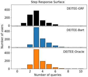
In addition to minimizing feature collection at test time with little to no loss in accuracy, DEITEE is able to person-alize the feature selection process, allowing different sub-populations to be asked a different number of questions. Fig-ure 2 is the histogram of the number of featFig-ures collected at test time showing significant variability in the number of features collected across the test population, thus conform-ing with insight 2 in the Preliminaries section.
Next, we inspect DEITEE’s ability to balance the accuracy-efficiency trade-off, where efficiency is measured by the number of unique features collected or queried at test time. We compare it to a more naive method of approaching
Figure 2: Histogram of the number of features collected by DEITEE at test time. Number of features collected varies: The majority of individuals require 3 features while few harder-to-estimate individuals require more.
this problem which relies on simple regularization. Specif-ically, we train the base model once using all the variables, compute the variable importance1then retrain the model
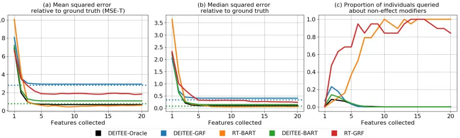
us-ing only the top k variables. We implement this approach for BART and GRF and refer to these retrained models as the RT-models. Figures 3(a) and 3(b) show the number of unique features collected on thex–axis and the correspond-ing MSE and Median SE on they–axis respectively. Plotted lines show performance of retrained models (RT-GRF and RT-BART), and DEITEE-distilled models (DEITEE-GRF and DEITEE-BART). Dotted lines show base model accu-racy.
We find that DEITEE-distilled methods have a lower mean and median squared errors after the first 2-3 queries. To understand the reason behind these gains in accuracy, we inspect the types of features that DEITEE collects and compare them to the retrained models. Figure 3(c) shows the number of unique features collected on thex−axis and the proportion of individuals queried about a variable that is not an effect modifier on the y−axis. We see that RT-BART tends to favor collecting effect modifiers in the first few rounds, neglecting to adjust for confounding while RT-GRF tends to collect non-effect modifiers perhaps prioritiz-ing adjustment for confoundprioritiz-ing at the expense of estimatprioritiz-ing heterogeneity. While the retrained methods continue asking additional questions which introduce marginal gains in ac-curacy, DEITEE stops after collecting non-effect modifiers from at most 20% of the population. This is an important feature: In non-simulated data, we would not be able to ob-serve accuracy plots similar to Fig 3(a,b) to pick thekwhere the error plateaus and subsequently retrain base models us-ing only thekmost important variables. In addition, we see that both the retraining method and DEITEE are able to
ex-1
Figure 3: DEITEE models achieve faster initial gains in accuracy, and tend to collect effect modifiers.
ploit the efficiency-accuracy trade-off; after a small number of variables is queried, the mean and median squared er-rors drop drastically and plateau after 5 or 6 questions. This number of questions is consistent with the number of vari-ables interacted with the treatment in these experiment set-tings. At the point where the models’ performances plateau, the MSE of the retrained methods are overall lower than those of the DEITEE-distilled model, however the median SE shows that the performance is overall comparable. The difference between the performance as measured through the mean and median errors suggests that the distribution over errors is skewed: for the majority of the population, DEITEE performs better than retraining but for some “hard” sub-populations, DEITEE gives less accurate estimates. Re-training improves estimates for these hard sub-populations but at the cost of collecting many more variables than neces-sary for the “easy” sub-populations, which DEITEE is able to avoid as shown in Figure 2.
Real data experiment
For our real data experiment, we show that DEITEE can en-able expecting mothers to plan and make decisions during their pregnancy based on how they might affect their babies’ health. Specifically, DEITEE can select the questions needed to ask the mother in order to ascertain the effect of differ-ent intervdiffer-entions and habits on the baby’s health. In such a scenario, collecting all the features (by asking the mother a barrage of questions) is not feasible, especially with vulnera-ble populations of pregnant women who most need the right medical advice. We explore two interventions: how initial-ization of perinatal care in the first trimesterandsmoking affect the baby’s health. We follow existing literature in us-ing the baby’s birth weight as an indicator of its health and well being (Almond, Chay, and Lee 2005). We use data from the 1989 Linked birth-infant death data which is made pub-licly available by the Centers for Disease Control (CDC ). The dataset has infant birth weight, as well as parent demo-graphics and mother risk factors for all 4 million babies born in the US. We restrict our analysis to the population of sin-gletons born in the state of Massachusetts (N = 91,065). We further drop any infants who are missing birth weight, mother’s smoking status or when she initialized her
perina-Table 2: DEITEE achieves large reductions in the features collected about soon-to-be-moms without loss of accuracy in estimating the effect of smoking and perinatal care on their babies’ birth weight.
Base DEITEE DEITEE DEITEE
MAE-P MAE-P MAE-B MVar
Smoking
BART 580.20 580.20 0.22 15.42 GRF 581.27 581.38 8.30 11.92 Perinatal care in the first trimester BART 587.62 587.62 0.26 16.20 GRF 588.03 588.06 3.13 15.70
tal care (N = 89,840). We split the data into 2/3 training and validation and 1/3 testing. Three-fold cross-validation is done to find the best parameters for the base model.
Here we do not have access to the true ITE so we cannot directly measure how well DEITEE or the base models do. Instead, we compute a proxy for the ITE by matching ev-ery mother in the test set with two similar mothers, one of whom belonged to the treatment group while the other does not. To find candidate matches, we use data from 1990 and data from 1989 from states other than Massachusetts. We identify the best matches as the ones having the smallest Eu-clidean distance relative to the features of the main mother. The proxy ITE is then computed as the difference between the birth weight of the baby belonging to the treated mother minus the birth weight of the baby of the control mother. We are able to match 76.1% for the perinatal care question and 70.0% for the smoking question.
We report MAE because it is in the same units as the treat-ment effect (change in birth weight in grams). Table 2 shows the mean absolute error of the base model relative to the proxy ITE (MAE-P), the MAE of DEITEE relative to the base model (MAE-B) and the mean number of features that were collected for mothers in the test set (Mvar). The results confirm our findings in semi-synthetic experiments: negligi-ble reductions in accuracy, and substantial reduction in the number of features required at test time.
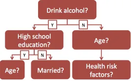
Figure 4: Decision tree stub distilling BART for the smoking question. Different feature paths are traversed for different mothers.
Figure 4 shows the first three questions asked by DEITEE upon distilling BART for the smoking question. DEITEE chooses to first ask women who consume alcohol about their education while for those who do not consume alcohol, it asks about age. When the treatment is starting perinatal care in the first trimester, DEITEE still chooses to ask women who consume alcohol about health risk factors while those who do not are asked about their marital status. Regardless of the treatment being studied, DEITEE always asks whether or not the mother consumes alcohol during her pregnancy signifying that that most variance in the treatment effect hinges on the mother’s alcohol consumption habits.
Conclusion
We presented DEITEE, a distillation method that enables accurate ITE estimation while demanding the collection of only a small number of variables at test time. Our approach exploits the fact that at training time both confounders and effect modifiers are required to accurately model the ITE while at test time only the effect modifiers are required to predict the ITE. Using 77 semi-synthetic datasets, we showed that DEITEE achieves significant reductions in the number of variables required at test time with little to no loss in accuracy. We demonstrated the utility of our approach us-ing real data. There are several specific areas of future work: More flexible models.While decision trees are appealing because of their simple and interpretable nature, they can be overly simplistic, and struggle to fit smooth response func-tions. Possible extensions to this work could explore more flexible function classes or hybrids of trees and more flexi-ble models such as GAMs.
Identification of Effect modifiers.In this work, we were concerned with collecting the smallest number of variables to accurately estimate the ITE. In other applications, we might wish to ensure that we only query effect modifiers, even if querying effect modifiers might require more vari-ables. Future work will focus on models which ask for the minimal number of effect modifiers.
References
Alaa, A. M., and van der Schaar, M. 2017. Bayesian inference of individualized treatment effects using multi-task gaussian pro-cesses. InAdvances in Neural Information Processing Systems, 3424–3432. Long Beach, USA: Curran Associates, Inc.
Alaa, A., and van der Schaar, M. 2018. Limits of estimating het-erogeneous treatment effects: Guidelines for practical algorithm
design. InProceedings of the 35th International Conference on Machine Learning, 129–138. Stockholm, Sweden: PMLR. Almond, D.; Chay, K. Y.; and Lee, D. S. 2005. The costs of low birth weight. The Quarterly Journal of Economics120(3):1031– 1083.
Athey, S., and Imbens, G. 2016. Recursive partitioning for hetero-geneous causal effects. Proceedings of the National Academy of Sciences113(27):7353–7360.
Athey, S.; Tibshirani, J.; and Wager, S. 2016. Generalized random forests. arXiv preprint arXiv:1610.01271. Forthcoming in Annals of Statistics.
Bucilua, C.; Caruana, R.; and Niculescu-Mizil, A. 2006. Model compression. In Proceedings of the 12th ACM SIGKDD Inter-national Conference on Knowledge Discovery and Data Mining, 535–541. Philadelphia, USA: ACM.
CDC. Linked birth and infant death data. https://www.cdc.gov/ nchs/nvss/linked-birth.htm.
Dorie, V.; Hill, J.; Shalit, U.; Scott, M.; and Cervone, D. 2017. Automated versus do-it-yourself methods for causal inference: Lessons learned from a data analysis competition. arXiv preprint arXiv:1707.02641.
Hill, J. L. 2011. Bayesian nonparametric modeling for causal inference. Journal of Computational and Graphical Statistics 20(1):217–240.
Johansson, F.; Shalit, U.; and Sontag, D. 2016. Learning repre-sentations for counterfactual inference. InProceedings of the 33rd International Conference on Machine Learning, 3020–3029. New York, USA: PMLR.
Kapelner, A., and Bleich, J. 2016. bartMachine: Machine learn-ing with Bayesian additive regression trees. Journal of Statistical Software70(4):1–40.
Lopez-Paz, D.; Bottou, L.; Sch¨olkopf, B.; and Vapnik, V. 2016. Unifying distillation and privileged information. InProceedings of the International Conference on Learning Representations, 26–36. Lou, Y.; Caruana, R.; and Gehrke, J. 2012. Intelligible models for classification and regression. InProceedings of the 18th ACM SIGKDD International Conference on Knowledge Discovery and Data Mining, 150–158. Beijing, China: ACM.
Pearl, J. 2009.Causality. Cambridge University Press.
Rosenbaum, P. R., and Rubin, D. B. 1983. The central role of the propensity score in observational studies for causal effects. Biometrika70(1):41–55.
Rosenbaum, P. R. 2002. Observational studies. InObservational studies. Springer. 1–17.
Rubin, D. B. 2005. Causal inference using potential outcomes. Journal of the American Statistical Association100(469):322–331. Shalit, U.; Johansson, F. D.; and Sontag, D. 2017. Estimating individual treatment effect: generalization bounds and algorithms. InProceedings of the 34th International Conference on Machine Learning, 3076–3085. Sydney, Australia: PMLR.
Spirtes, P., and Glymour, C. 1991. An algorithm for fast recovery of sparse causal graphs. Social science computer review9(1):62– 72.
Tibshirani, J.; Athey, S.; Wager, S.; Friedberg, R.; Miner, L.; and Wright, M. 2018. grf: Generalized Random Forests (Beta). R package version 0.10.1.