R E S E A R C H
Open Access
The interval versions of the Kalman filter and
the EM algorithm
O Al-Gahtani
1*, J Al-Mutawa
2, M El-Gebeily
2and R Agarwal
1,3*Correspondence:
[email protected] 1Department of Mathematics, King
Saud University, Riyadh, Kingdom of Saudi Arabia
Full list of author information is available at the end of the article
Abstract
In this paper, we study state space models represented by interval parameters and noise. We introduce an interval version of the Expectation Maximization (EM) algorithm for the identification of the interval parameters of the system. We also introduce a suboptimal interval Kalman filter for the identification and estimation of the state vectors. The work requires the introduction of the concept of interval random variables which we also include in this work together with a study of their interval statistical properties such as expectation, conditional expectation and variance. Although the interval Kalman filter introduced here is suboptimal, it successfully recovers the state vectors to a high precision in the simulation examples we have run.
1 Introduction
In a state space model, some parameters of the system such as the coefficient matrices may not be precisely known or they gradually change with time. One way to account for these uncertainties is to allow such parameters to be represented by interval entities. The ques-tion then arises as to how to extend identificaques-tion and estimaques-tion techniques to interval settings.
To our knowledge, no attempt has been made so far to extend identification techniques such as the EM algorithm to interval state space models. In this work, we give one such an extension.
In the existing literature, an optimal interval Kalman filter was attempted in []. That attempt suffered from the lack of proper definitions and rigorous treatment. The idea in [] was to replace the interval system setting with the ‘worst case inversion’ while keeping everything else unchanged. So, the ultimate treatment in [] amounts to the application of the traditional Kalman filter to the system representing the worst case scenario. This way the authors were able to avoid the difficulties that arise when dealing with interval arithmetic and concepts. On the other hand, this algorithm cannot be called optimal and the concept of the optimal interval Kalman filter remains an open question.
In our work, we introduce a spacial interval arithmetic that always produces results that are smaller (in the sense that it is contained) than the traditional interval arithmetic [, ]. This arithmetic enables the extension of the Kalman filter as well as the EM algorithm to interval setting in a true sense. In our restricted interval arithmetic, the interval Kalman filter we introduce here is optimal. However, with respect to the more general interval arithmetic, our interval Kalman filter is suboptimal.
2 A special interval arithmetic
We introduce a special set of interval operations that will enable the extension of the usual linear system concepts to the interval setting in a seamless manner. The more general definitions of the interval operations can be found in []. The arithmetic introduced here avoids such vague terms as ‘interval extension’, ‘inclusion function’, determinantsetc.that have been used in the literature [, –].
All the interval operations adopted in this work stem from the view of an interval as a set of convex combinations of its endpoints:
I= [a,b] =xα= ( –α)a+αb:α∈[, ]
.
Definition SupposeI= [a,b],J= [c,d] are intervals and• ∈ {+, –,∗,÷}. Define the fol-lowing interval operations:
I•J=xα•yα:α∈[, ],xα∈I,yα∈J
,
with the usual restriction /∈Jif•=÷.
Observe that all operations in Definition result in intervals since they can be regarded as continuous functions defined on the unit interval [, ]. For example, a typical element inI∗Jis ( –α)ac+α( –α)(ad+bc) +αbdwhich is a continuous function ofα. The operations in Definition give similar results to the usual interval operations as given in [] when• ∈ {+, –}, but generally they give only subintervals if• ∈ {∗,÷}. For example, ifI= [–, ], thenI∗I= [, ] according to Definition , while the usual definition in [] givesI∗I= [–, ].
The operations in Definition are associative:
I+ (J+K) = (I+J) +K,
I∗(J∗K) = (I∗J)∗K and distributive:
I∗(J+K) =I∗J+I∗K.
For example, distributivity is shown as follows:
I∗(J+K) =Iα(J+K)α:α∈[, ]
=Iα(Jα+Kα) :α∈[, ]
=IαJα+IαKα:α∈[, ]
=(IJ)α+ (IK)α:α∈[, ]
=(IJ+IK)α:α∈[, ]
=IJ+IK.
the other hand, these definitions were motivated by our attempt to arrive at a definition of interval random variables and investigate the corresponding statistical properties. We feel that they are the natural ones to handle interval systems. This feeling is reassured by the numerical results we obtained in the simulation examples (see Section ). While we expected to obtain a construction of a suboptimal interval Kalman filter, the constructed filter was actually able to recover the exact simulated intervals rather than subintervals.
Interval vectors and matrices are defined similarly: • A vectorv∈IRnis defined as
v= [a,b] =xα= ( –α)a+αb:α∈[, ], where
a,b∈Rn, a≤b,
and the inequality holds componentwise. • A matrixA∈IRn×nis defined as
A= [A,B] =Xα= ( –α)A+αB:α∈[, ]
,
where
A,B∈Rn×n, A≤B,
and the inequality holds componentwise.
Definition Given a functionf:Rk→Rnand an interval vectorv∈IRk, we define
f(v) =f(xα) :α∈[, ]
.
Iffis continuous, thenf(v) is an interval vector. All operations on functions are extended to interval settings in the same way. For example,
fg(v) =f(v)g(v) =f(xα)g(xα) :α∈[, ]
,
df dv=
df
dxα :α∈[, ]
,
provided that the involved operations make sense. In the same spirit, interval matrix op-erations are defined as follows:
• The interval determinant is defined by
det(A) =det(Xα) :α∈[, ]
.
• The interval adjoint is defined by
adj(A) =adj(Xα) :α∈[, ]
• The interval inverse is defined by
A–=Xα–:α∈[, ]
=
adj(Xα)
det(Xα)
:α∈[, ]
=adj(A)
det(A).
The continuous dependence of the determinant of a matrix on the elements of the matrix implies that all the above operations produce interval entities. Naturally, these special definitions produce results that are contained in the corresponding usual definitions. To give an example, we use the definition of the inverse interval matrix
A–according to []:
A–=X–:X∈A,
where[S]is the smallest interval vector (matrix) containingS. If
A=
[] [–, ] [–, ] [] ,
then
S=X–:X∈A=
–rs –
r
–rs
––rrs –rs :r,s∈[–, ]
.
One can show that the set of points inRwith coordinates equal to the first row of the elements ofSforms a polygonal (non-rectangular) region with vertices at(,), (, ),(,),(, –),(, –). Thus,
A–= [S] =
[,] [–,] [–,] [,] .
The inverse in our sense is
A–=
[,] [,] [,] [,] .
• Suppose thatA–exists. We define the solution of the interval linear systemAX=bto be
X=X∈Rn:AαX=bα,α∈[, ]
.
Clearly,Xis an interval vector. The usual definition is
Obviously, our definition produces a smaller interval vector. In fact, ifA–exists in the sense of [], then
X⊂S⊂[S]⊂A–b.
The last inclusion holds because ifX∈S, then there is anA∈Aand ab∈bwithAX=b. ThenX=A–b∈A–b⊂A–b. Thus,S⊂A–b. Noting thatA–bis an interval vector and [S] is minimal, we get that [S]⊂A–b.
For the rest of this paper, we will use the special interval operations defined above. Finally, for error estimates, we need to introduce the distance between two intervals I= [a,b],J= [c,d]. This is defined by
q(I,J) :=max|a–c|,|b–d|.
The mapqdefines a metric inIR.
3 Interval random variables
We begin by discussing the measurability of set-valued maps and then introduce the defi-nition of an interval random variable. The basic defidefi-nitions and more details can be found in []. A measurable space (,A) consists of a basic settogether with aσ-algebraA of subsets ofcalled measurable sets. Here, we consider closed convex value set-valued mapsF:⇒Rk,i.e.,F(ω) is a closed convex subset ofRkfor eachω∈. This is the case
whenFis interval valued. The latter notion means that for eachω∈, the components ofF(ω) are closed intervals inR.
We first define what it means for a set-valued map to be measurable. Recall that the inverse image of a setS⊂Rkunder the set-valued mapFis defined by
F–(S) =ω∈:F(ω)∩S=∅,
and that the graph ofF(denoted byGF) is defined by
GF=
(ω,y) :ω∈,y∈F(ω).
Definition Let (,A) be a measurable space andF:⇒Rkbe a set-valued map.Fis
called measurable if the inverse image of each open set is a measurable set: ifO⊂Rkis
open, thenF–(O)∈A.
We are now in a position to introduce the definition of interval random variables and interval stochastic processes.
Definition Let (,S,P) be a probability space. An interval-valued mapX:⇒Rkis called an interval random variable if
. Xis measurable, and
. the functionx→pxis continuous onX, wherepxis the probability density function
for the random variablex.
The probability density functionpXis then the interval-valued function
pX={px:x∈X}.
In order to study the expectations and variances of interval random variables, we need to discuss first the integral of set-valued maps and, in particular, interval-valued maps. The discussion begins with the notion of measurable selections.
Definition Let (,A) be a measurable space andF:⇒Rkbe a measurable set-valued
map. A measurable selection ofFis a measurable mapf :→Rksatisfyingf(ω)∈F(ω) for eachω∈.
It is well known that every measurable set-valued map has at least one measurable se-lection []. Furthermore, we have the following equivalences [].
Theorem Let(,A)be a measurable space and denote byBtheσ-algebra of Borel sets
inRk.Let F:⇒Rkbe a set-valued map.The following are equivalent. . Fis measurable.
. GF∈A⊗B.
. F–(B)∈Afor everyB∈B.
. There exists a sequence of measurable selections{fn}∞n=ofFsuch that
F(ω) =
n≥ fn(ω)
for eachω∈.
A countable family of measurable selections satisfying the last property is calleddense. LetF:⇒Rkbe an interval-valued map. We define the two special functionslFandrF
such thatlF(ω) =a(ω) andrF(ω) =b(ω), whereF(ω) = [a(ω),b(ω)] for eachω∈. The next
lemma shows thatlF andrFare measurable selections ofFwhen the latter is measurable.
Lemma Let F:⇒Rkbe a measurable interval-valued map.Then the point functions lFand rFare measurable selections of F.
Proof Choose a sequence of measurable selections{fn}∞n=ofFsuch that
F(ω) =
n≥ fn(ω).
ThenlF(ω) =infn≥fn(ω) andrF(ω) =supn≥fn(ω) (here theinfandsupoperations are taken
componentwise). Since theinfand thesupoperators preserve measurability, we see that the functionslFandrF are measurable selections ofF.
Example Let= [,∞) and defineF:⇒Rby
F(t) =
t,t+ t
Let{rn}∞n= be an enumeration of the rational numbers in the interval [, ], and let us
A measurable selectionf ofFis an integrable selection iff is integrable with respect to the measureμ. The set of all integrable selections ofFwill be denoted byF. The mapFis called integrably bounded if there exists aμ-integrable functiong∈L(;R,μ) such that F(ω)⊂g(ω)Bforμ-almost everyω∈. Here,Bdenotes the unit ball inRk. In this case, every measurable selectionf ofFis also an integrable selection sincef(ω)∈F(ω)⊂g(ω)B
implies thatf(ω) ≤ |g(ω)|, where · denotes the Euclidean norm onRk.
Definition The integral of a set-valued mapFis defined to be the set of integrals of integrable selections ofF. That is,
We shall say thatFis integrable if every measurable selection is integrable.
We have the following immediate properties:
On the other hand, let θ ∈ [lFdμ,
The second equality is an immediate consequence of this.
It will always be assumed that bothlFandrF are integrable.
Example LetandFbe defined as in the previous example. Letμbe the measure defined by
In view of (), we have the following corollary.
Corollary Let F,F:⇒Rkbe integrable interval-valued maps.Then
We shall say thatZisnormally distributedif eachz∈Zis normally distributed. An in-terval stochastic process{Zt}t∈Twill be called normally distributed if for eacht∈T,Ztis
normally distributed.
LetZbe an interval random variable. Then for eachz∈Z, plz≤pz≤prz.
By the continuity ofz→pz,
This means that
lpZ=plz, rpZ=prz.
Guided by this and Lemma , we can define theinterval expectationof the interval random variableZas follows.
Definition The interval expectation of an interval random variableZis defined as
E(Z) =E(lZ),E(rZ)
.
This definition coincides with Definition since
E(lZ),E(rZ)
=αE(lZ) + ( –α)E(rZ) :α∈[, ]
=EαlZ+ ( –α)rZ
:α∈[, ] =E(zα) :α∈[, ]
.
It should also be noted that the expectation of a vector random variable is the vector of expectations of its components.
It follows from equations () and () that
E(λZ) =λE(Z),
E(Z+Z) =E(Z) +E(Z).
Also, ifI= [a,b] andZis an interval random variable, then
E(IZ) =E(tαzα) :α∈[, ]
=tαE(zα) :α∈[, ]
=I∗E(zα) :α∈[, ]
=IE(Z).
The same is true ifIis an interval vector andZis an interval random variable.
More generally, if Ais a k×k interval matrix and if its columns are denoted by the interval vectorsA,A, . . . ,Ak, then
E(AZ) =E k
j=
AiZj
=
k
j=
E(AiZj) = k
j=
AiE(Zj)
=AE(Z).
To introduce covariance of two interval random variablesY,Z, we need to assume that the function (x,y)→px,yis continuous onY×Z. Here,px,yis the joint probability density
Definition The interval covariance of two interval random variablesY,Zis defined as
Cov(Y,Z) =Cov(yα,zα) :α∈[, ]
.
To see thatCov(Y,Z) is an interval, note that
Cov(Y,Z) =Cov( –α)lY+αrY, ( –α)lZ+αrZ
:α∈[, ] =( –α)Cov(lY,lZ) +α( –α)Cov(lY,rZ)
+α( –α)Cov(rY,lZ) +αCov(rY,rZ) :α∈[, ]
.
IfY=Z, we get the definition of the variance of an interval random variableZas
Var(Z) =Var(zα) :α∈[, ]
=( –α)Var(lZ) + α( –α)Cov(lZ,rZ) +αVar(rZ) :α∈[, ]
which is also an interval. Elementary calculus considerations reveal that
Var(Z) =
ab–c
a+b– c,max{a,b}
,
wherea=Var(lZ),b=Var(rZ),c=Cov(lZ,rZ). This last equation provides a formula for
computing the intervalVar(Z).
For interval random vectors, the above definitions hold componentwise.
The two interval random variablesY,Zwill be called uncorrelated if for eachyα∈Y,
zα∈Z,yα,zαare uncorrelated. Therefore,Y,Zare uncorrelated if and only ifCov(Y,Z) =
[].
It is now straightforward to check the following theorem.
Theorem LetY,Z∈IRk,W∈IRm,IRnbe interval random vectors,and letA∈IRk×k,
B∈IRm×m,λ∈IR,then . Cov(λY,W) =λCov(Y,W),
. Cov(Y+Z,W) =Cov(Y,W) +Cov(Z,W), . Cov(AY,BW) =ACov(Y,W)BT.
The assumed continuous dependence of the probability density function (joint density function) on the random variable (variables) in an interval random variable (interval ran-dom variables) implies that the conditional probability density function is also continuous. This guarantees that the generalization of the conditional density function to the interval setting is always an interval.
Definition The interval conditional expectation is defined as
E(Z|Y) =E(zα|yα) :α∈[, ]
=αE(lZ|yα) + ( –α)E(rZ|yα) :α∈[, ]
The following theorem is easily checked.
Theorem For vector random variablesX,Y,Zand interval matrixAof appropriate dimensions,
. E(X+Y|Z) =E(X|Y) +E(Y|Z), . E(AY|Z) =AE(Y|Z).
4 The interval state space model
The interval state space model we will consider here is one of the form
xt+=Axt+wt, ()
yt=Hxt+vt, t≥, ()
whereA∈IRk×k,H∈IRp×kare interval matrices andwt∈IRk,vt∈IRpare zero-mean
Gaussian white-noise interval processes, with
Cov
wt vt
,
ws vs
=
Q R δts,
while the initial statexis assumed to be an interval random variable having zero-mean, interval variance matrix and to be uncorrelated to{wt}and{vt} for allt≥. The
matricesQ∈IRk×k,R∈IRp×pare also allowed to be interval matrices. For the time being, we assume that the matricesF,H,Q,Rare knowna priori. We thus have the properties
Cov(wt,xs) =, Cov(vt,xs) =, s≤t,
Cov(wt,yt) =Q, Cov(vt,yt) =R.
For the state covariance matrix
t=Cov(xt,xt),
we have the recursion
t+=AtAT+Q, t≥
with initial value.
4.1 The interval Kalman filter
In this section, we give a summary of the interval settings of the Kalman filter and the EM algorithm. The ground work that we did in the previous two section should reveal that it is possible to apply both methods to interval state space models. LetYs={y,y, . . . ,ys}be
a sequence of interval measurements up to timesand let
The expectation is a forecast fors<t, a filtered value fors=tand a smoothed value for s>t. The least square estimation error is defined by
Pst=Ext–xst
xt–xst
T
.
The interval Kalman filter is defined in two main steps: estimation and forecast [, ]. The estimation step is given by
xtt–=Axtt––, Ptt–=APtt––AT+Q,
and the forecast step is given by
xtt=xtt––+Kt
yt–Hxtt––
, ()
Ptt= (I–KtH)Ptt–, t= , , . . . ,n, ()
where
Kt=Ptt–
HPtt–HT+R–
is called the Kalman gain. The initial conditions arex=μandP=.
The interval Kalman smoother, which is needed for the EM algorithm, is defined by
xnt =xtt+Jt
xnt+–xtt+, ()
Pnt =Ptt+Jt
Pnt+–Ptt+JTt, ()
where
Jt=PttAT
Ptt+–.
The initial conditionsxn
nandPnnin this case are found from () and (). The EM
algo-rithm also needs the so-called lag-one covariance smoother defined by
Pnn,n–= (I–KnH)APnn––,
Pnt,t–=PttJTt–+JTtPnt+,t–APttJTt–, t=n– ,n– , . . . , .
()
.. The EM algorithm in interval setting
The EM algorithm [–] tries to estimate the parameter set={A,H,Q,R}of the sys-tem (), () by maximizing the likelihood of its probability density functionP(x,). The algorithm consists of two steps, the expectation step (E-step) and the maximization step (M-step). The E-step uses the current available parameter setto obtain estimates for the state vector and the least square error. This step is based on the Kalman filter and Kalman smoother. The M-step uses the current estimated values of the state vector and errors to obtain a new parameter set according to the equations
A=CB–, ()
Q= n
H=SD–, ()
The method can be summarized as follows.
. Initialize the procedure by selecting starting values for the elements of the parameter set()={A(),H(),Q(),R()}and estimateμ
.
. (E-step) Forj= , , . . ., use the parameter set(j–)to estimate the smoothed values
xnt,Pnt,Pnt,t–(equations ()-()) fort= , , . . . ,n.
. (M-step) Calculate a new set of parameters(j)using equations ()-(). . Repeat steps and above until convergence is achieved.
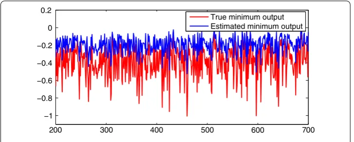
5 Simulation results
A Monte Carlo simulation is performed to illustrate the utility of the interval EM al-gorithm estimate. The observed data are generated according to the second order interval state space model
wherewtandvtare independent identically distributed (i.i.d.) Gaussian noises such that
wt∼N
This model is a slightly modified version of the one used in []. In all simulations, the number of iterations for the EM algorithm is fixed atJ= . We used theα values of α = : . : for the interval estimates. Figure shows a sample of realizations of the
minimum, true and maximum observed output dataytrespectively, while Figure shows
Figure 1 Output signals.
Figure 2 Estimated output signals.
Figure 3 Maximum observed and estimated output signals.
(MSE):
EN=
N
N
t=
(yt–Cxt|t–)
Figure 4 Minimum observed and estimated output signals.
Competing interests
The authors declare that they have no competing interests.
Authors’ contributions
The authors have achieved equal contributions to each part of this paper. All authors read and approved the final version of the manuscript.
Author details
1Department of Mathematics, King Saud University, Riyadh, Kingdom of Saudi Arabia.2Department of Mathematics and
Statistics, King Fahd University of Petroleum and Minerals, Dhaharan, 31261, Kingdom of Saudi Arabia.3Department of Mathematics, Texas A&M University-Kingsville, Kingsville, TX 78363-8202, USA.
Acknowledgements
Dr. O. Al-Gahtani extends his appreciation to the Research Center of Teachers College, King Saud University for funding his work through the research group project No. RGP-TCR-07. The second and third authors would like to thank King Fahd University of Petroleum and Minerals for the excellent research facilities they provide.
Received: 2 May 2012 Accepted: 14 September 2012 Published: 2 October 2012
References
1. Chen, G, Wang, J, Shieh, LS: Interval Kalman filtering. IEEE Trans. Aerosp. Electron. Syst.33(1), 250-259 (1997) 2. Alefeld, G, Herzberger, J: Introduction to Interval Computations. Academic Press, San Diego (1983) 3. Rohn, J: Inverse interval matrix. SIAM J. Numer. Anal.3, 864-870 (1993)
4. Bentbib, AH: Conjugate directions method for solving interval linear systems. Numer. Algorithms21, 79-86 (1999) 5. Kubica, BJ, Malinowski, K: Interval random variables and their application in queueing systems with long-tailed
service times. In: SMPS, pp. 393-403 (2006)
6. Chen, W, Tan, S: Robust portfolio selection using interval random programming. In: FUZZ-IEEE, Korea, 2009, August 20-24 (2009)
7. Aubin, J-P, Frankowska, H: Set-Valued Analysis. Birkhäuser, Basel (1990)
8. Ekland, I, Témam, R: Convex Analysis and Variational Problems. Classics in Applied Mathematics, vol. 28. SIAM, Philadelphia (1999)
9. Jazwinski, A: Stochastic Precesses and Filtering Theory. Academic Press, New York (1970) 10. Tanizaki, H: Nonlinear Filtering: Estimation and Applications. Springer, Berlin (1996)
11. Bilms, JA: A gentle tutorial of the EM algorithm and its applications to parameter estimation for Gaussian mixture and hidden Markov models. Technical report TR-97-021, ICSI (1997)
12. Dempster, AP, Laird, NM, Rubin, DB: Maximum likelihood from uncomplete data via the EM algorithm. J. R. Stat. Soc. B
39, 1-38 (1977)
13. Shumway, RH, Stoffer, DS: An approach to time series smoothing and forecasting using the EM algorithm. J. Time Ser. Anal.3(4), 253-264 (1982)
14. Shumway, RH, Stoffer, DS: Time Series Analysis and Its Applications. Springer, Berlin (2006)
doi:10.1186/1687-1847-2012-172