27 Abstract-The aim of the project is getting into a new level in the
field of Image processing by 3D volume calculation of brain tumor using image processing techniques. The image is Pre-operated based on pixel intensities by using Gaussian filter. Then the images are segmented using clustering technique by K-means algorithm. Thus the brain images are partitioned as a gray matter, white matter, Cerebro Spinal Fluid (CSF) and Tumor. Tumor features are extracted using Histogram of oriented gradients (HOG) and the Brain tumor is classified using Support Vector Machine technique. The 2D image of the brain tumor is detected and the 2D image is converted into 3D image using connected-components where, connected component technique is used to detect the viewing points for creating the 3D image. Then the volume of the tumor is calculated.
Key words-pre-operated, k-means, Brain tumor, pixel intensities, Histogram of oriented gradients.
I INTRODUCTION:
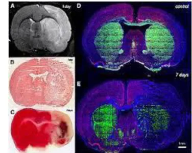
For atlas seeding, Expectation Maximization algorithm incorporates with glioma growth model. Atlas seeding is a process which differentiates tumor and edema from original atlas as shown in the
figure 1
.
For estimation tumor model parameters from the patient’s scans the atlas registration and low-dimensional description gives a good result in addition to segmentation..For various results tumor and edema differentiated which gives the similar accuracy[1].
Figure 1. Output image for GLISTR
M.Raghavi, UG Scholar, Department of Electronics and Communication Engineering, Kalasalingam University, Tamilnadu, India. (Mail id: [email protected]).
M.Princy, UG Scholar, Department of Electronics and Communication Engineering, Kalasalingam University, Tamilnadu, India (Mail id: [email protected]).
R.Priyanka, UG Scholar, Department of Electronics and Communication Engineering, Kalasalingam University, Tamilnadu, India.(Mail Id: [email protected]).
Mrs.A.Lakshmi, Assistant Professor, Department of Electronics and Communication Engineering, Kalasalingam University, Tamilnadu, India(Mail id: [email protected]).
To reduce the flow estimates on their initial valuesa novel optical flow estimation method is proposed. Adaption of the objective function and development of a new optimization procedure is included. The effectiveness of this method is borne out by experiments for both large- and small-displacement optical flow estimation in the figure 2[2].
Figure 2. Output image preserving optical flow estimation
In standard clinical cases, a large number of multi-modal and multi-temporal image volumes is acquired requiring new approaches for comprehensive integration of information from different image sources and different time points. Here the method proposed was a joint generative model of tumor growth of image observation that naturally handles multimodal and longitudinal data, by this model patient’s glioma was analyzed thus the output gives Generative approach for image based modeling of tumor growth as shown in the figure3 [3].
Figure 3. A Generative approach for image based modeling of tumor growth
”DRAMMS” is referred as deformable registration algorithm. DRAMMS was used in the traditional voxel-wise methods and landmark/feature-based methods, different registration task can be applied, regardless of the image contents under registration. DRAMMS second characteristic is based on a cost function that
M.Raghavi, M.Princy, R.Priyanka, Mrs.A.Lakshmi
3D Volume Calculation of Brain Tumor Using Hog
Feature Extraction and Connected Component
Technique
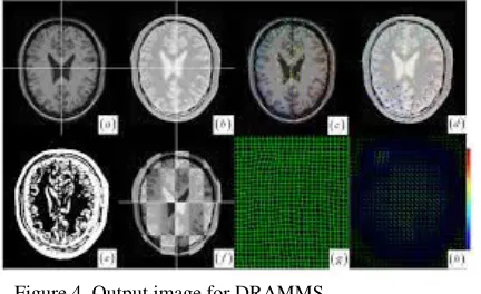
28 weights different voxel pairs according to a ”mutual-saliency”, which
reflects the reliability of anatomical correspondences implied by the tentative transformation as given in the figure 4. The optimization process, do not contribute image voxels at the result. similar to the methods like binary selection fashion or voxel-wise methods as in
most feature-based methods[4]
.
Figure 4. Output image for DRAMMS
(IT) non-rigid registration algorithms based on L2 and information-theory is exactly symmetric, which pair the same points of two images after the images are swapped. But L2 and IT non-rigid registration algorithms are only approximately symmetric. Because of the objective function and the numerical techniques used in discretizing and minimizing the objective functions. For eliminating both sources of asymmetry many techniques are provided, an infinite-dimensional space of such graph-based forms is given [5]. II PROPOSED METHOD
The proposed system consists of five modules: Pre-processing, segmentation, feature extraction, classification and volume calculation. Pre-processing is carried out by filtering using windowed filter. The process of segmentation is done by K-means algorithm. Feature extraction is done by Histogram Oriented Gradients (HOG). Finally, Volume of the brain tumor is calculated using connected components. In the existing methods many types of segmentation are used but they are all not good for all types of MRI images.
2. Proposed method block diagram
Figure 5. Block diagram of proposed method
Fig 5 is the block diagram of proposed method. It consists of six modules. Each module and its function will be explained below.
2.1. PRE-PROCESSING A. Pre-processing description:
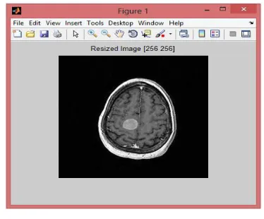
In this module initially, the input image is given as shown in the figure 6 and the given image is resized to the standard size of 256 as shown in the figure 8 and the noise is removed from the image. In Filtering, Gaussian filtering is used to the input image. Mostly, Gaussian filtering is used to remove the noise from the image as shown in the figure 8. Here wiener2 function is used to the to the input image. Gaussian filter is a windowed filter which is named after famous scientist Carl Gauss, weights in the filter calculated according to Gaussian distribution. Naturally it is a weighted mean and a linear class.
B. Gaussian filter algorithm:
1. Given window size 2N+1 calculate support points x=3n/N, n=-N, -N+1, ... , N;
Calculate values G";
Calculate scale factor k'=∑G";
Calculate window weights G'=G"/k';
For every signal element:
Place window over it;
Pick up elements;
Multiply elements by corresponding window weights;
Sum up products — this sum is new filtered value.
Figure 6. Input MRI image
Segmentation
Pre-procesin g
Feature extraction SVM
classifier Tumor
detection
Volume calculation
29
Figure 7. Resized image
Fig7. is resized image to the standard size of 256
Figure 8. Output image for Pre-processing
Fig8. is the output image for removing noise from the resized image using Gaussian filter in Pre-processing.
2.2. SEGMENTATION
Here the image is clustered by the use of k-means algorithm. It is the algorithm which is used for partitioning the images. K cluster centers are found and objects are assigned to the nearest cluster center as shown in the figure 10. Such that, it minimizes the squared distance of the cluster as shown in the . K-means clustering is a method of vector quantization originally from image processing that is popular for cluster analysis in images. To model the data they both use cluster centers; however, the expectation maximization mechanism allows clusters to have different shapes while k-means clustering tends to find clusters of comparable spatial extent. The K-means algorithm can easily be used for this task and produces competitive results.
2.3. K-MEAN ALGORITHM A.K-means algorithm description:
Vector quantization method involves K-means clustering cluster analysis in data mining is more popular in signal processing. K-means clustering aims to partitioned observations into k clusters in which each observation belongs to the cluster with the nearest mean, served as a cluster’s prototype.
B. Mathematical Representation:
Given a set of observations (x1, x2, …, xn), where each observation is a
dimensional real vector. The main objective of the K-means clustering is to partitioned n observations into k clusters (k ≤ n) S = {S1, S2, …, Sk}. so as to minimize the within-cluster sum of
squares (WCSS):
---(1)
Where μi is the mean of points in Si.
Given an initial set of k means m1(1),…,m2(1)
C. Algorithm:
1. Give the value as K for no of clusters. 2. Choose K random centers.
3. For each cluster calculate the mean of centre.
4. Determine the distance between each pixel & cluster centre. 5. If the distance is nearer to that centre then move to the same cluster. 6. Or else move it to the next cluster.
7. Estimate the clustered image
8. Repeat the same process until the center does not moves.
Figure 9. Output images for K-means clustering.
Fig9. is the output image clustered into gray matter, white matter, CSF and tumor using K-means algorithm.
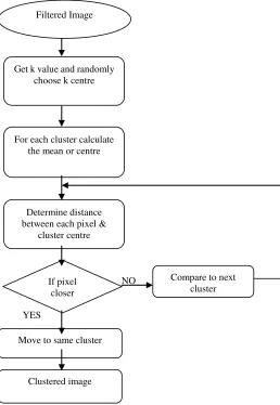
30 D. Flow chart of K-mean Algorithm
NO
YES
Figure 10 . Flow chart for K-means clustering
2.4. HOG FEATURE EXTRACTION
In HOG, Local binary pattern is a technique of feature descriptors used for the purpose of object detection in computer vision and image processing. The HOG feature is extracted here. It is called Histogram of Oriented Gradients. Localized portions of an image, occurrences of gradient orientation count by this technique as shown in the figure 11. This method resembles scale-invariant feature transform descriptors, the edge orientation histograms and shape contexts but differs with computed on a dense grid of equally spaced cells and uses overlapping local contrast normalization for improved accuracy. Here the two steps involved are as follows:
1. Computation of the gradient values.
2. Creating the cell histograms
.
1. Computation of the gradient values:
By applying the 1-D centered, point discrete derivative mask in one or both of the vertical and horizontal directions which is a most common method used. Specifically, this method needs, filtering the color or image’s intensity data.
2. Creating the cell histograms:
Cell in the each pixel casts a weighted vote for an orientation-based histogram channel depend on the values rectangular in shape, and the histogram channels are uniformly spread over 0 to 180 degrees or 0 to 360 degrees, based on whether the gradient is “signed” or “unsigned”. Screenshot for HOG Feature extraction:
Figure 11. Output for HOG Feature Extraction
Fig11.is the extracted features using gradient values in an image. From this tumor features are extracted and trained by SVM.
2.5. TUMOR DETECTION
For tumor Identification, here the SVM classifier is used to identify the tumor in image. One of the supervised classifier is SVM classifier. Here the technique used is Kernel-based which represents a major development in machine learning algorithms. The feature values are provided to the SVM classifier . The feature will trained by the classifier. Finally the result will be classified as shown in the figure 12. Based on the training data (predicts the target values), model of the SVM is produced. The test data attributes is given only by the target values of the test data.
A. SVM Classification description:
An optimal hyper plane is constructed using SVM maps input vectors which is a higher dimensional vector space. Among the many hyper planes available, there is only one hyper plane called the optimal separating hyper plane that maximizes the distance between itself and the nearest data vectors of each category. To the closest training vectors of each category the hyper plane which maximizes the margin as the sum of distances.
B. Mathematical Expression:
Expression for hyper plane
w.x+b = 0 ---(2) x – Set of training vectors
Filtered Image
Get k value and randomly choose k centre
For each cluster calculate the mean or centre
Determine distance between each pixel &
cluster centre
Move to same cluster
Clustered image If pixel
closer
31 w – Vectors perpendicular to the separating hyper plane
b – Offset parameter which allows the increase of the margin C. Algorithm:
(i) Data setup: Dataset consists of three classes, each N samples. For visual inspection the data is 2D plot of original data.
(ii) SVM with linear kernel (-t 0). The best parameter value C can be find by using 1/2 data to train, the other 1/2 to test which is called as 2-fold cross validation.
(iii)The best parameter value for C is found, and then the entire data will be trained using this parameter value.
(iv) Plot support vectors. (v) Plot decision area.
Screenshot for tumor detection:
Figure 12. Output image for tumor detection
The SVM trained the image to detect the tumor and then the tumor detected to all the given images.
2.6. VOLUME CALCULATION
A. Volume Calculation Description:
The volume of the tumor is calculated based on the Connected Components. Connected-component can also used to detect the connected regions in color images, although digital images and data which having higher dimensionality can also be processed. One of the most common operations in machine vision. It finds all connected components in an image and assigns a unique label to all the points in a component. After finding the region it is created as 3D image and then the volume of the tumor is calculated from the segmented result as sown in the figure 12.
B. Algorithm:
Step 1: Start the Process.
Step 2: Get the MRI input image in jpeg format.
Step 3: Get the standard size of an image from the input MRI image. Step 4: Pre-process the image
Step 5: Segment the image using clustering Step 6: Identify the tumor
Step 7: Calculate the viewing points using connected components. Step 8: Calculate the Volume of the tumor using the formula Step 9: Display the output image.
Step 10: Stop the program
Figure 12. Output image for 3D tumor evaluation and tumor volume calculation.
Fig12 is the Output for conversion of 3D using connected component and then the volume of the 3D is calculated.
III CONCLUSION
Initially the region is clusterd by clustering algorithm. After that feature is extracted by HOG feature extraction to predict the tumor region. The extracted HOG features passed to the SVM classifier to train about the tumor in the images. Then the tumor region is segmented using K-mean clustering. And finally it passed to the 3D volume calculation. This technique provides the better performance and also the segmentation accuracy also high.
IV FUTURE ENHANCEMENT
32 REFERENCES
[1]. A. Gooya, K. M. Pohl, M.Billell, “Glioma image segmentation and registration”, IEEE Trans .Med. Imag.,Nov 2011.
[2]. L.Xu, J. Jia, and Y.Matsushita; ”Motion detail preserving optical flow estimation”; IEEE Transactions on Pattern Analyses and Machine Intelligence;vol.34:9; 2012.
[3]. B.H.Menze, K. V. Leemput, A. Honkela, Konukoglu, M.A.Weber, N. Ayache, and P. Golland , “A generative approach for image-based modeling of tumor growth” Inf Process Med
Imaging;vol.22. pp.735-47,2011.
[4].Y. Ou, A. Sotiras, N. Paragios, and C. Davatzikos, “DRAMMS: Deformable registration via attribute matching and mutual-saliency weighting”,Medical Image analyses ; vol.15(4); pp.622-39; Aug 2011.
[5]. H. D. Tagare, D. Groisser, and O. M. Skrinjar; “A geometric theory and some numerical techniques”, J Math Imaging;34; 61-88;2009.
[6] B. L. Dean, B. P. Drayer, C. R. Bird, R. A. Flom, J. A. Hodak, S. W. Coons, and R. G. Carey, “Gliomas: Classification with MR Imaging,” Radiology, vol. 174, no. 2, pp. 411–415, 1990.
[7] S. Periaswamy and H. Farid, “Medical image registration with partial data,” Med. Image Anal., vol. 10, no. 3, pp. 452–464, 2006. [8] N. Chitphakdithai and J. S. Duncan, “Non-rigid registration with missing correspondences in preoperative and postresection brain images,” in Proc. MICCAI, vol. 6361, pp. 367–374, 2010.
[9] M. Niethammer, G. L. Hart, D. F. Pace, P. M. Vespa, A. Irimia, J. D. V. Horn, and S. R. Aylward, “Geometric
metamorphosis,” in Proc. MICCAI, vol. 6892, pp. 639–646,2011. [10] O. Clatz, H. Delingette, I.-F. Talos, A. Golby, R. Kikinis, F. A. Jolesz, N. yache, and S. K.Warfield, “Robust nonrigid registration to capture brain shift from intraoperativeMRI,” IEEE Trans. Med. Imag., vol. 24,no. 11, pp. 1417–1427, Nov. 2005.
[11] P. Risholm, E. Samset, I.-F. Talos, andW.Wells, “A non-rigid registration framework that accommodates resection and retraction,” in Proc. Inf. Process. Med. Imag., vol. 5636, pp. 447–458,2009. [12] A. Mohamed, E. I. Zacharaki, D. Shen, and C. Davatzikos, “Deformable registration of brain tumor images via a statistical model of tumor-induced deformation,” Med. Image Anal., vol. 10, no. 5, pp. 752–763, 2006.
[13] E. I. Zacharaki, D. Shen, S.-K. Lee, and C. Davatzikos, “ORBIT: A multiresolution framework for deformable registration of brain tumor images,” IEEE Trans. Med. Imag., vol. 27, no. 8, pp. 1003–1017, Aug. 2008.
[14] M. Prastawa, E. Bullitt, S. Ho, and G. Gerig, “A brain tumor segmentation framework based on outlier detection,” Med. Image Anal., vol. 8, no. 3, pp. 275–283, 2004.