Volume 3, Issue 3, March 2014
Page 339
Abstract
Bathymetric data is depth values of reservoir. Bathymetric data is useful for hydrographic survey, volume calculation and 3D plot generation. Echo sounder collects bathymetric data using ultrasonic waves. Using interpolation techniques 3D plot is obtained. Noise gets added during reflection of ultrasonic waves from bottom of reservoir in SONAR system. Ultrasonic data taken from SONAR is not accurate because noise gets added and there is need to remove noise. To remove noise there is need to know type of noise present in ultrasonic data. Type of noise is found out using statistical analysis of data. Histogram analysis is preferred to identify noise type and then by applying noise removal algorithm noise is removed. After removing noise, we can estimate more accurate volume of reservoir.
Keywords: Echo Sounder, data interpolation, 3D plot, statistical Analysis, Noise removal algorithm.
1.
I
NTRODUCTIONMountains occupy 24% of the global land surface area and are home to 12% of the world’s population. About 10% of the world’s population depends directly on the use of mountain resources for their livelihoods and wellbeing and an estimated 40% depends indirectly on them for water, hydroelectricity, timber, biodiversity, niche products, mineral resources, recreation and flood control [1].
Reservoirs are a major part of the usable surface water resources They are used for multiple purposes, including water supply, recreation, flood control, sports fishery, industrial purposes, and hydroelectric-power generation.
Accumulation of sediment is one of the most serious factors that threaten aquatic environments such as reservoirs, lakes and ponds. Sedimentation causes some lakes, ponds and reservoirs to be filled and polluted within a short time. It also causes loss of area and volume, and reduces the lifespan of facilities. Due to sediment accumulation reflection of ultrasonic waves adds noises in ultrasonic data.
Echo sounder is instrument which is used for generating ultrasonic data [2]. Noise gets added during reflecting ultrasonic wave from bottom of reservoir in SONAR system. Noise is any undesired information that degrades the image and appears in images from a variety of sources. The goal of denoising is to remove the noise while retaining the important signal features to the extent possible, and can be done through filtering of different type [3-5]. Histogram analysis is also preferred to identify noise type.
2.
DATA
INTERPOLATION
Interpolation methods are used here to calculate the unknown heights of interested points in reservoir by referring to the elevation information of neighboring points. These gridding methods are used to interpolate irregularly spaced XYZ data into a regularly spaced grid.
The different gridding methods are inverse distance to a power, kriging, minimum curvature, modified Shepard’s method, natural neighbor, nearest neighbor, polynomial regression, radial basis function, and triangulation with linear interpolation, moving average, data metrics, and local polynomial. There are total twelve gridding methods used to interpolate data. Triangulation with linear interpolation contains TIN algorithm. Triangulated Irregular Networks algorithm consist of following steps
A. Topological Relations of TIN Establishing
Compared with the simple data structure of Grid, the data structure of TIN is much more complex. Topological relations allow data structures of TIN are classified into: point structure, surface structure, point-surface structure, edge structure and edge-surface structure.
B. Survey Area Splitting
It is unacceptable to construct the Delaunay triangulation with the huge amount of data points directly. A proper way is splitting the survey area into several sub-blocks first, and then constructing Delaunay triangulations individually.
C. Delaunay Triangulation Construction
The algorithms of Delaunay triangulation construction can be divided into several groups: divide & conquer, incremental insertion, incremental construction, sweeping and high-dimensional embedding. We adopt the incremental insertion algorithm for Delaunay triangulation for reasons of its simplicity, robustness and acceptable speed.
D. Sub-triangulations Merging
Performance Analysis Different Filters for Noise
Removal of Underwater Bathymetric Data
Anjali Ghadage1, Selva Balan2 and Sushama Shelke3
1
Student, Dept. of E&TC, NBN Sinhgad School of Engineering, Pune, India.
2Chief resech officer, Cwprs, khadakwasla,Pune, India. 3
Volume 3, Issue 3, March 2014
Page 340
Sub-triangulations are merged in reverse order of splitting, that means merge the leaf nodes in binary tree in descending order according to the level.
3.
DATA STATISTICS
Estimations for the most common statistics that are used in hydrological estimations, predictions and testing are studied. Data statistics are used here to know type of noise present in data. It is assumed that the sample is a time series of length n whose items to time instances, i.e.
X
1 …,X
n .3.1 Mean
This is arithmetic average of the x values and is usually referred to simply as the mean. The formulae for mean are as follows:
n X
n
i
X
I
1 (1)
Here n is length of samples and samples is taken for time instant
X
1 toX
n and i is from 1,2,….n.3.2 Median
Median is the middle value of the given numbers or distribution in their ascending order. Median is the average value of the two middle elements when the size of the distribution is even.
3.3 Variance
Variance measures how far each number in the set is from the mean.
Variance is calculated by taking the differences between each number in the set and the mean, squaring the differences (to make them positive) and dividing the sum of the squares by the number of values in the set.
n
i
X
x
S
in 1
2
2
(
)
1 1
(2)
Here n is length of samples and samples is taken for time instant
X
1 toX
n and i is from 1,2,….n, X is mean.3.4 Standard deviation
The sample standard deviation is the square root of the mean squared difference between each observation and the sample mean; it is defined by the left-most formula above. This formula is awkward for hand computations, but minimizes round off errors. The equation is usually reorganized into the form on the right for hand calculations.
S
S 2 (3)
Here
S
2 is variance.3.5 Histogram
Histogram is a graphical display of data using bars of different heights.
The histogram condenses a data series into an easily interpreted visual by taking many data points and grouping them into logical ranges or bins.
4.
NOISE PATTERNS
Noise pattern is plot of histogram for different noises with few random numbers. Underwater data contains uniform noise, Gaussian noise, salt and pepper noise and speckles noise.
4.1 Uniform noise
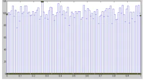
Uniform noise is not often encountered in real-world imaging systems, but it provides a useful comparison with Gaussian noise. The linear average is comparatively poor estimator for the mean of a uniform distribution. This implies that nonlinear filters should be better to removing uniform noise than Gaussian noise. Fig.1 shows the histogram of uniform noise pattern [6].
Volume 3, Issue 3, March 2014
Page 341
4.2 Gaussian noise
The Gaussian distribution has an important property that in order to estimate the mean of a stationary Gaussian random variable, one can’t do any better than the linear average. This makes Gaussian noise worst-case scenario for nonlinear image restoration filters, in the sense that the improvement over linear filters is least for Gaussian noise. To improve on linear filtering results, nonlinear filters can exploit only the non- Gaussianity of the signal distribution. Fig.2 shows the histogram of Gaussian noise pattern with 10000 random numbers [6].
Figure 2 Gaussian noise pattern
4.3 Impulse noise
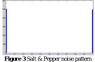
Impulsive noise is sometimes called as salt-and-pepper noise or spike noise. An image containing salt-and-pepper noise will have dark pixels in bright regions and bright pixels in those dark regions. This type of noise can be caused by dead pixels, analog-to digital converter errors, bit errors in transmission etc.
) , ( ) , ( ) ,
(I j y I j w I j
f (4)
Original data y(i, j), w(i, j) be the noisy data and f(i , j) is the noisy. Fig.3 shows the histogram of impulse noise pattern with equal probabilities [6].
Figure 3 Salt & Pepper noise pattern
4.4 Speckle Noise
Another common form of noise is data drop-out noise generally referred to as speckle noise. This noise is, in fact, caused by errors in data transmission .The corrupted pixels are either set to the maximum value, which is something like a snow in image or have single bits flipped over.
) , ( ) , ( ) ,
(I j y I j w I j
f (5)
Original data y(i, j), w(i, j) be the noisy data and f(i , j) is the noisy. Fig.4 shows the histogram of speckle noise pattern [6].
Figure 4 Speckle noise pattern
5.
NOISE REMOVING FILTER
5.1 Median filter
Volume 3, Issue 3, March 2014
Page 342
Median filter(x1….xN) =Median (||x1||…….||xN||) (6)
Fig.5 shows image plotted after applying median filter but it does not give proper results.
Figure 5 Image from bathymetric data after Median filtering
5.2 Gaussian Filter
Gaussian low pass filter is the filter which is impulse responsive, Gaussian filters are designed to give a no overshoot to a step function input while minimizing the rise and fall time. Gaussian is smoothing filter in the 2D convolution operation that is used to remove noise.
Fig.6 shows plot after applying Gaussian filter but it also does not give proper results.
Figure 6 Image from bathymetric data after Gaussian filtering
6.
EXPERIMENTAL RESULTS
All experiments were carried out using Matlab 7.0 simulations.
A. Data collation
A Personal Computer was connected to the Sonar through a serial data cable to access the operating system of the instrument and to download the data for post processing applications. Geographical Positioning System (GPS) was connected to the Sonar using a standard data cable, so that GPS readings were generated in conjunction with instrument’s echo sounding functions to create full XYZ hydrographic data using Sonar software package.
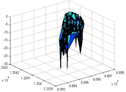
B. 3D Plot
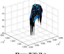
After data collection that data is plotted using TIN algorithm which contains Delaunay triangulation. Triangulated Irregular Networks, this is algorithm for interpolation of bathymetric data. In this algorithm contain four steps which are topological Relations of TIN establishing in this relation are established then survey area splitting and then delaunay triangulation Construction in this incremental insert algorithm is used then Sub-triangulations Merging 3D plot which is reconstructed using TIN algorithm is easy to compare with Surfer 8.
Figure 7 3D Plot
Volume 3, Issue 3, March 2014
Page 343
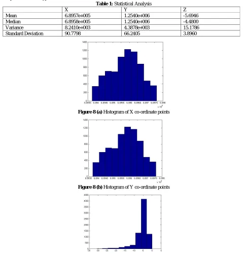
C. Statistical analysis
Statistical analysis is done to know type of noise. Mean, median, variance, standard deviation is calculated and histogram is plotted to know type of noise.
Table 1: Statistical Analysis
X Y Z
Mean 6.8957e+005 1.2540e+006 -5.6946
Median 6.8958e+005 1.2540e+006 -4.4800
Variance 8.2410e+003 4.3878e+003 15.1786
Standard Deviation 90.7798 66.2405 3.8960
Figure 8 (a) Histogram of X co-ordinate points
Figure 8 (b) Histogram of Y co-ordinate points
Figure 8 (c) Histogram of Z co-ordinate points
Table I shows values of mean, median, variance and standard deviation. And fig.8 (a), fig.8 (b), fig.8 (c) Histogram of X Y Z co-ordinate points. From statistical analysis and histogram plot we came to conclusion that data contain Gaussian noise.
D. Noise removal
Volume 3, Issue 3, March 2014
Page 344
Figure 9 3D plot after filtering
7.
CONCLUSION
Bathymetric data is plotted using TIN algorithm in MATLAB which show that data contain noise. Statistical analysis of ultrasonic data and histogram of each column of ultrasonic data shows that data contains Gaussian noise so there is need to apply filter on data. By applying median filter and Gaussian filter not much amount of noise gets removed. So after smoothing data then apply median which gives better results. After filtering, ultrasonic data set image is reconstructed using TIN algorithm but that images consists of triangles and that is not proper 3D plot so in future by using image enhancement techniques proper image is recovered and then accurate volume is calculated.
REFERENCES
[1] Schild, “The case of the Hindu Kush–Himalayas: ICIMOD’s position on climate change and mountain systems”, Mountain Research and Development, March, 2008.
[2] Mohd Ansor Bin Yusof, Shahid Kabir, “Underwater Communication Systems: A Review”, Progress In Electromagnetics Research Symposium Proceedings, Marrakesh, Morocco, pp.803-807, March, 2011.
[3] Hassen M. Yesuf, Tena ,Alamirew, Assefa M. Melesse and Mohammed Assen, “Bathymetric Mapping for Lake Hardibo in Northeast Ethiopia Using Sonar”, International Journal of Water Sciences, pp.1-9, August, 2012.
[4] Demetris Koutsoyiannis, “Climate change, the Hurst phenomenon, and hydrological statistics”, Hydrological Sciences–Journal–des Sciences Hydrologiques, pp. 1-24, February, 2003.
[5] Sang-Ki Moon, Nam C. Woo, Kwang S. Lee, “Statistical analysis of hydrographs and water-table fluctuation to estimate groundwater recharge”, Journal of Hydrology, pp. 198–209, December, 2004.
[6] Shamik Tiwari, Ajay Kumar Singh, V.P. Shukla, “Statistical Moments based Noise Classification using Feed Forward Back Propagation Neural Network”, International Journal of Computer Applications , Volume 18– No.2, pp.36-40, March 2011.
[7] Dan Lu, Haisen Li, Yukuo Wei, TongxiShen, “An Improved Merging Algorithm for Delaunay Meshing on 3D Visualization Multibeam Bathymetric Data”, Proceedings of the 2010 IEEE International Conference on Information and Automation, pp. 1171-1176, June, 2010.
[8] Padmavathi, Subashini, Muthu Kumar and Suresh Kumar Thakur, “Performance analysis of Non Linear Filtering Algorithms for underwater images” , (IJCSIS) International Journal of Computer Science and Information Security, Vol.6, No. 2, pp. 232-238, June, 2009.
[9] Pierre Cervenka and Christian de Moustier, “Post processing and Corrections of Bathymetry Derived from Sidescan Sonar Systems :Application with SeaMARC II”, IEEE Journal of Oceanic Engineering, Vol.19, No. 4, pp. 619-629, October 1994.