Regularized Estimation and Testing
for High-Dimensional Multi-Block Vector-Autoregressive Models
Jiahe Lin [email protected]
Department of Statistics University of Michigan Ann Arbor, MI 48109, USA
George Michailidis∗ [email protected]
Department of Statistics and the Informatics Institute University of Florida
Gainesville, FL 32611, USA
Editor:Jie Peng
Abstract
Dynamical systems comprising of multiple components that can be partitioned into distinct
blocks originate in many scientific areas. A pertinent example is the interactions between financial assets and selected macroeconomic indicators, which has been studied ataggregate level—e.g. a stock index and an employment index—extensively in the macroeconomics literature. A key shortcoming of this approach is that it ignores potential influences from other related components (e.g. Gross Domestic Product) that may impact the system’s dynamics and structure and thus produces incorrect results. To mitigate this issue, we con-sider a multi-block linear dynamical system with Granger-causal ordering between blocks, wherein the blocks’ temporal dynamics are described by vector autoregressive processes and are influenced by blocks higher in the system hierarchy. We derive the maximum likelihood estimator for the posited model for Gaussian data in the high-dimensional setting based on appropriate regularization schemes for the parameters of the block components. To optimize the underlying non-convex likelihood function, we develop an iterative algorithm with convergence guarantees. We establish theoretical properties of the maximum likeli-hood estimates, leveraging the decomposability of the regularizers and a careful analysis of the iterates. Finally, we develop testing procedures for the null hypothesis of whether a block “Granger-causes” another block of variables. The performance of the model and the testing procedures are evaluated on synthetic data, and illustrated on a data set involving log-returns of the US S&P100 component stocks and key macroeconomic variables for the 2001–16 period.
Keywords: Vector-autoregression; Stability; Block-coordinate descent; Consistency; Global testing
1. Introduction.
The study of linear dynamical systems has a long history in control theory (Kumar and Varaiya,1986) and economics (Hansen and Sargent,2013) due to their analytical tractability and ease to estimate their parameters. Such systems in their so-called reduced form give
∗. Corresponding Author. Post Address: 205 Griffin Floyd Hall, 1 University Ave, Gainesville, FL, 32611.
c
rise to Vector Autoregressive (VAR) models (L¨utkepohl,2005) that have been widely used in macroeconomic modeling for policy analysis (Sims,1980,1992), in financial econometrics (Gourieroux and Jasiak, 2001), and more recently in functional genomics (Shojaie et al., 2012), financial systemic risk analysis (Billio et al.,2012) and neuroscience (Seth,2013).
In many applications, the components of the system under consideration can be nat-urally partitioned into interacting blocks. For example, Cushman and Zha (1997) studied the impact of monetary policy in a small open economy, where the economy under consid-eration is modeled as one block, while variables in other (foreign) economies as the other. Both blocks have their own autoregressive structure, and the inter-dependence between blocks is unidirectional: the foreign block influences the small open economy, but not the other way around, thus effectively introducing a linear orderingamongst blocks. Another example comes from the connection between the stock market and employment macroe-conomic variables (Fitoussi et al., 2000; Phelps, 1999; Farmer, 2015) that focuses on the impact through a wealth effect mechanism of the former on the latter. Once again, the underlying hypothesis of interest is that the stock market influences employment, but not the other way around. In another application domain, molecular biologists conduct time course experiments on cell lines or animal models and collect data across multiple molecular compartments (transcripotmics, proteomics, metabolomics, lipidomics) in order to delineate mechanisms for disease onset and progression or to study basic biological processes. In this case, the interactions amongst the blocks (molecular compartments) are clearly delineated (transciptomic compartment influencing the proteomic and metabolomic ones), thus leading again to a linear ordering of the blocks.
The proposed model also encompasses the popular in marketing, regional science and growth theory VAR-X model, provided that the temporal evolution of theexogenousblock of variables “X” exhibits autoregressive dynamics. For example,Nijs et al. (2001) examine the sensitivity of over 500 product prices to various marketing promotion strategies (the exogenous block), while Pauwels and Weiss (2008) examine changes in subscription rates, search engine referrals and marketing efforts of customers when switched from a free account to a fee-based structure, the latter together with customer characteristics representing the exogenous block. Pesaran et al. (2004) examine regional inter-dependencies, building a model where country specific macroeconomic indicators evolve according to a VAR model and they are influenced exogenously by key macroeconomic variables from neighboring countries/regions. Finally, Abeysinghe (2001) studies the impact of the price of oil on Gross Domestic Product growth rates for a number of countries, while controlling for other exogenous variables such as the country’s consumption and investment expenditures along with its trade balance.
xt−1
yt−1
zt−1
xt
yt
zt
xt+1
yt+1
zt+1 timet
timet−1 timet+ 1
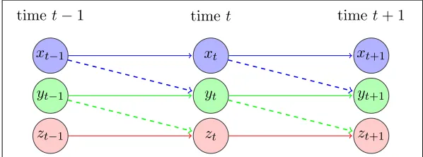
Figure 1: Diagram for a dynamic system with three groups of variables
Given the wide range of applications of multi-block VAR models, which in addition encompass the widely used VAR-X model, the key contributions of the current paper are fourfold: (i) formulating the model as a recursive dynamical system and examining its stabil-ity properties; (ii) developing a provably convergent algorithm for obtaining the regularized maximum likelihood estimates (MLE) of the model parameters under high-dimensional scal-ing; (iii) establishing theoretical properties of the ML estimates; and (iv) devising a testing procedure for the parameters that connect the constituent blocks of the model: if the null hypothesis is not rejected, then one is dealing with a set of independently evolving VAR models, otherwise with the posited multi-block VAR model. Finally, the model, estima-tion and testing procedures are illustrated on an important problem in macroeconomics, as gleaned by the background of the problem and discussion of the results provided in Section6.
For the multi-block VAR model, we assume that the time series within each block are generated by a Gaussian VAR process. Further, the transition matrices within and across blocks can be eithersparseorlow rank. The posited regularized Gaussian likelihood function is notjointly convex in all the model parameters, which poses a number of technical chal-lenges that are compounded by the presence of temporal dependence. These are successfully addressed and resolved in Section3, where we provide a numerically convergent algorithm and establish the theoretical properties of the resulting ML estimates, that constitutes a key contribution in the study of multi-block VAR models.
The remainder of this paper is organized as follows. In Section2, we introduce the model setup and the corresponding estimation procedure. In Section 3, we provide consistency properties of the obtained ML estimates under a high-dimensional scaling. In Section 4, we introduce the proposed testing framework, both for low-rank and sparse interaction matrices between the blocks. Section 5 contains selected numerical results that assess the performance of the estimation and testing procedures. Finally, an application to financial and macroeconomic data that was previously discussed as motivation for the model under consideration is presented in Section6.
Notation. Throughout this paper, we use |||A|||1 and |||A|||∞ respectively to denote the matrix induced 1-norm and infinity norm ofA∈Rm×n, that is,|||A|||
1 = max1≤j≤n Pm
respec-tively. For two matrices Aand B of commensurate dimensions, denote their inner product by hhA, Bii= trace(A0B). Finally, we writeA%B if there exists some absolute constant c
that is independent of the model parameters such thatA≥cB.
2. Problem Formulation.
To convey the main ideas and the key technical contributions, we consider a recursive linear dynamical system comprising of two blocks of variables, whose structure is given by:
Xt=AXt−1+Ut,
Zt=BXt−1+CZt−1+Vt,
(1)
where Xt ∈ Rp1, Zt ∈Rp2 are the variables in groups 1 and 2, respectively. The temporal
intra-block dependence is captured by transition matrices A and C, while the inter-block dependence by B. Noise processes {Ut} and {Vt}, respectively, capture additional contem-poraneous intra-block dependence ofXt andZt, after conditioning on their respective past values. Further, we assume that Ut and Vt follow mean zero Gaussian distributions with covariance matrices given by Σu and Σv, i.e.,
Ut∼ N(0,Σu), and Vt∼ N(0,Σv).
With the above model setup, the parameters of interest are transition matricesA∈Rp1×p1,
B ∈Rp2×p1 andC∈
Rp2×p2, as well as the covariances Σu,Σv. In high-dimensional settings, different combinations of structural assumptions can be imposed on these transition matrices to enable their estimation from limited time series data. In particular, the intra-block transition matricesAand Care sparse, while the inter-block matrixB can be either sparse or low rank. Note that the block ofXtvariables acts as anexogenouseffect to the evolution of the Zt block (e.g., Cushman and Zha, 1997; Nicolson et al., 2016). Further, we assume Ωu:= Σ−u1 and Ωv := Σ−v1 are sparse.
Remark 1 For ease of exposition, we posit a VAR(1) modeling structure. Extensions to general multi-block structures akin to the one depicted in Figure1andVAR(d)specifications are rather straightforward and briefly discussed in Section 7.
The triangular (recursive) structure of the system enables a certain degree of separability between Xt and Zt. In the posited model, Xt is a stand-alone VAR(1) process, and the time series in block Zt is “Granger-caused” by that in block Xt, but not vice versa. The second equation in (1), as mentioned in the introductory section, also corresponds to the so-called “VAR-X” model in the econometrics literature (e.g., Sims, 1980; Bianchi et al., 2010), that extends the standard VAR model to include influences from lagged values of
exogenousvariables. Consider the joint processWt= (Xt0, Zt0)0, it corresponds to a VAR(1) model whose transition matrix Ghas a block triangular form:
Wt=GWt−1+εt, where G:=
A O
B C
, εt=
Ut
Vt
. (2)
structural VAR representation with Granger causal ordering (L¨utkepohl, 2005). As men-tioned in the introductory section, the focus of this paper is model parameter estimation under high-dimensional scaling, rather than their cause and effect relationship. For a com-prehensive discourse of causality issues for VAR models, we refer the readers to Granger (1969);L¨utkepohl(2005), and references therein.
Next, we introduce the notion of stability and spectrum with respect to the system.
System Stability. To ensure that the joint process {Wt} is stable (L¨utkepohl, 2005), we require the spectral radius, denoted by ρ(·), of the transition matrix G to be smaller than 1, which is guaranteed by requiring that ρ(A)<1 andρ(C)<1, since
|λIp1×p2 −G|=
λIp1−A O −B λIp2 −C
=|λIp1 −A||λIp2−C|,
implying that the set of eigenvalues ofGis the union of the sets of eigenvalues of Aand C, hence
ρ(A)<1, ρ(C)<1, ⇒ ρ(G) = max{ρ(A), ρ(C)}<1.
The latter relation implies that the stability of such a recursive system imposes spectrum constraints only on the diagonal blocks that govern the intra-block evolution, whereas the off-diagonal block that governs the inter-block interaction is left unrestricted.
Spectrum of the joint process. Throughout, we assume that the spectral density of {Wt} exists, which then possesses a special structure as a result of the block triangular transition matrix G. Formally, we define the spectral density of{Wt}as
fW(θ) = 1 2π
∞
X
h=−∞
ΓW(h)e−ihθ, θ∈[−π, π],
where ΓW(h) :=EWtWt0+h. For two (generic) processes {Xt}and {Zt}, define their cross-covariance as ΓX,Z(h) =EXtZt0+h and ΓZ,X(h) =EZtXt0+h. In general, ΓX,Z(h)6= ΓZ,X(h). The cross-spectra are defined as:
fX,Z(θ) := 1 2π
∞
X
h=−∞
ΓX,Z(h)e−ihθ, and fZ,X(θ) := 1 2π
∞
X
h=−∞
ΓZ,X(h)e−ihθ, θ∈[−π, π].
For the model given in (2), by writing out the dynamics of Zt, the cross-spectra between
Xtand Zt are given by
fX,Z(θ)(Ip2 −C 0
e−iθ) =fX(θ)B0e−iθ, and (Ip2−Ce iθ)f
Z,X(θ) =BeiθfX(θ). (3)
Similarly, we have
(Ip2 −Ce iθ)f
Z(θ) =BeiθfX,Z(θ) +fV,Z(θ). (4)
Combining (3) and (4), the spectrum of the joint processWtis given by
fW(θ) =
H1(eiθ)
−1
H2(eiθ)
12×2⊗fX(θ)
H2(e−iθ)
> +
O O
O Σv
H1(e−iθ)
−>
where12×2 is a 2×2 matrix with all entries being 1, and
H1(x) :=
Ip1 O
O Ip2 −Cx
∈R(p1+p2)×(p1+p2), H2(x) :=
Ip1 O
O Bx
∈R(p1+p2)×(2p1).
Equation (5) implies that the spectrum of the joint process {Wt} can be decomposed into the sum of two parts: the first, is a function of fX(θ), while the second part involves the idiosyncratic error process{Vt}, which only affects the right-bottom block of the spectrum. Note that since {Wt} is a VAR(1) process, its matrix-valued characteristic polynomial is given by
G(θ) := I(p1+p2)−Gθ,
and its spectral density also takes the following form (c.f.Hannan,1970):
fW(θ) = 1 2π
G−1(eiθ)Σε
G−1(eiθ)∗,
where
G(x) =
Ip1 −Ax O −Bx Ip2 −Cx
, Σε =
Σu O
O Σv
,
and G∗ is the conjugate transpose. One can easily reach the same conclusion as in (5) by multiplying each term, followed by some algebraic manipulations.
2.1 Estimation.
Next, we outline the algorithm for obtaining the ML estimates of the transition matrices
A, B and C and inverse covariance matrices Σ−u1 and Σ−v1 from time series data. We allow for a potential high-dimensional setting, where the ambient dimensions p1 and p2 of the model exceed the total number of observations T.
Given centered times series data {x0,· · ·, xT} and {z0,· · · , zT}, we use XT and ZT respectively, to denote the “response” matrix from time 1 to T, that is:
XT =x1 x2 . . . xT 0
and ZT =z1 z2 . . . zT 0
,
and use X and Z without the superscript to denote the “design” matrix from time 0 to
T−1:
X =
x0 x1 . . . xT−1 0
and Z =
z0 z1 . . . zT−1 0
.
We use U and V to denote the error matrices. To obtain estimates for the parameters of interest, we formulate optimization problems using a penalized log-likelihood function, with regularization terms corresponding to the imposed structural assumptions on the model parameters–sparsity and/or low-rankness. To solve the optimization problems, we employ block-coordinate descent algorithms, akin to those described inLin et al. (2016), to obtain the solution.
As previously mentioned, {Xt} is not “Granger-caused” byZt and hence it is a stand-alone VAR(1) process; this enables us to separately estimate the parameters governing the
Estimation of A and Σ−u1. Conditional on the initial observation x0, the likelihood of {xt}Tt=1 is given by:
L(xT, xT−1,· · ·, x1|x0) =L(xT|xT−1,· · · , x0)L(xT−1|xT−2,· · · , x0)· · ·L(x1|x0) =L(xT|xT−1)L(xT−1|xT−2)· · ·L(x1|x0),
where the second equality follows from the Markov property of the process. The log-likelihood function is given by:
`(A,Σ−u1) = T
2 log det(Σ −1 u )−
1 2
T X
t=1
(xt−Axt−1)0Σu−1(xt−Axt−1) + constant.
Letting Ωu := Σ−u1, then the penalized maximum likelihood estimator can be written as (A,b Ωbu) = arg min
A∈Rp1×p2
Ωu∈S++p1×p1 n
tr
Ωu(XT− XA0)0(XT− XA0)/T−log det Ωu+λAkAk1+ρukΩuk1,off
o
. (6)
Algorithm 1describes the key steps for obtaining Aband Ωbu.
Algorithm 1:Computational procedure for estimating Aand Σ−u1. Input: Time series data {xt}Tt=1, tuning parameterλA andρu.
1 Initialization: Initialize withΩb (0)
u = Ip1, then
b
A(0) = arg minA1 T
XT − XA0 2
F +λAkAk1 ;
2 Iterate until convergence:
– Update Ωb (k)
u by graphical Lasso (Friedman et al.,2008) on the residuals with the plug-in estimateAb(k);
– Update Ab(k) with the plug-in Ωb (k−1)
u and cyclically update each row with a Lasso penalty, which solves
min A
1 Ttr
b
Ω(uk−1)(XT − XA)0(XT − XA)/T
+λAkAk1 . (7) Output: Estimated sparse transition matrix Aband sparse Ωbu.
Estimation of B, C and Σ−1
v . Similarly, to obtain estimates ofB, C and Ωv := Σ−v1, we
formulate the optimization problem as follows:
(B,b C,b Ωbv) = arg min B∈Rp2×p1,C∈Rp2×p2
Ωv∈S++p2×p2 n
trΩv(ZT − XB0− ZC0)0(ZT − XB0− ZC0)/T
−log det Ωv
+λBR(B) +λCkCk1+ρv||Ωv||1,off
o
, (8)
Algorithm 2:Computational procedure for estimating B,C and Σ−v1.
Input: Time series data {xt}Tt=1 and{zt}Tt=1, tuning parameters λB,λC,ρv.
1 Initialization: Initialize withΩb (0)
v = Ip2, then
(Bb(0),Cb(0)) = arg min (B,C)
1 T
ZT − XB0− ZC0 2
F +λBR(B) +λCkCk1 .
2 Iterate until convergence:
– Update Ωb (k)
v by graphical Lasso on the residuals with the plug-in estimates Bb(k) andCb(k);
– For fixedΩb (k)
v , (Bb(k+1),Cb(k+1)) solves min
B,C 1
Ttr
b
Ω(vk)(ZT − XB0− ZC0)0(ZT − XB0− ZC0)+λBR(B) +λCkCk1 .
·FixCb[s], updateBb[s+1] by Lasso or singular value thresholding, which solves min
B 1
Ttr
b
Ω(vk)(ZT − XB0− Z
b
C[s]0)0(ZT − XB0− Z
b
C[s]0)
+λBR(B) ;
·FixBb[s], updateCb[s]by Lasso, which solves min
C 1
Ttr
b
Ω(vk)(ZT − XBb[s] 0
− ZC0)0(ZT − XBb[s] 0
− ZC0)+λCkCk1 . Output: Estimated transition matrices Bb,Cb and sparse Ωbv.
and Ωbv. Note thatBb(k) andCb(k) need to be treated as a “joint block” in the outer update and convergence of the “joint block” is required before moving on to updating Ωv.
Note that the objective function in (6) is notjointly convexin both parameters, but biconvex. Similarly in (8), the objective function is biconvex in(B, C),Ωv
. Consequently, convergence to a stationary point is guaranteed, as long as estimates from all iterations lie within a ball around the true value of the parameters, with the radius of the ball upper bounded by a universal constant that only depends on model dimensions and sample size (Lin et al.,2016, Theorem 4.1). This condition is satisfied upon the establishment of consistency properties of the estimates.
To establish consistency properties of the estimates requires the existence of good initial values for the model parameters (A,Ωu), and (B, C,Ωv), respectively, in the sense that they are sufficiently
close to the true parameters. For the (A,Ωu) parameters, the results inBasu and Michailidis(2015)
guarantee that for random realizations of {Xt, Et}, with sufficiently large sample size, the errors
of Ab(0) and Ωb
(0)
u are bounded with high probability, which provides us with good initialization
values. Yet, additional handling of the bounds is required to ensure that estimates from subsequent iterations are also uniformly close to the true value (see Section3.2Theorem5). A similar property for (Bb(0),Cb(0),Ωb
(0)
v ) and subsequent iterations is established in Section 3.2 Theorem 6 (see also
Theorem15in AppendixA).
3. Theoretical Properties.
estimates. We focus on the model specification in which the inter-block transition matrix B is
low rank, which is of interest in many applied settings. Specifically, we consider the consistency properties ofAband (B,b Cb) that are solutions to the following two optimization problems:
(A,b Ωbu) = arg min A,Ωu
n tr
Ωu(XT − XA0)0(XT − XA0)/T−log det Ωu+λAkAk1+ρukΩuk1,off
o
, (9)
and
(B,b C,b Ωbv) = arg min B,C,Ωv
n tr
Ωv(ZT− XB0− ZC0)0(ZT− XB0− ZC0)/T−log det Ωv
+λB|||B|||∗+λCkCk1+ρv||Ωv||1,off
o
.
(10)
The case of a sparseB can be handled similarly to that of Aand/or C with minor modifi-cations (details shown in Supplementary Material??).
3.1 A road map for establishing the consistency results.
Next, we outline the main steps followed in establishing the theoretical properties for the model parameters. Throughout, we denote with a superscript “?” the true value of the corresponding parameters.
The following key concepts, widely used in high-dimensional regularized estimation prob-lems, are needed in subsequent developments.
Definition 2 (Restricted Strong Convexity (RSC)) For some generic operator X :
Rm1×m2 7→ RT×m1, it satisfies the RSC condition with respect to norm Φ with curvature αRSC >0 and tolerance τ >0 if
1
2T|||X(∆)|||
2
F ≥αRSC|||∆|||2F −τΦ2(∆), for some ∆∈Rm1
×m2.
Note that the choice of the norm Φ is context specific. For example, in sparse regression problems, Φ(∆) =k∆k1corresponds to the element-wise`1norm of the matrix (or the usual vector `1 norm for the vectorized version). The RSC condition becomes equivalent to the
restricted eigenvalue (RE) condition(seeLoh and Wainwright,2012;Basu and Michailidis, 2015, and references therein). This is the case for the problem of estimating transition matrix A. For estimating B and C, define Q to be the weighted regularizer Q(B, C) := |||B|||∗+λC
λBkCk1, and the associated norm Φ in this setting is defined as
Φ(∆) := inf
Baug+Caug=∆Q(B, C).
Definition 3 (Diagonal dominance) A matrixΩ∈Rp×p is strictly diagonally dominant if
|Ωii|> X
j6=i
|Ωij|, ∀ i= 1,· · ·, p.
Definition 4 (Incoherence condition (Ravikumar et al., 2011)) A matrixΩ∈Rp×p
satisfies the incoherence condition if:
max
e∈(SΩ)ckHeSΩ(HSΩSΩ)
−1k
where HSΩSΩ denotes the Hessian of the log-determinant barrier log det Ω restricted to the
true edge set of Ω denoted by SΩ, and HeS is similarly defined.
The above two conditions are associated with the inverse covariance matrices Ωu and Ωv. Specifically, the diagonal dominance condition is required for Ω?u and Ω?v as we build the consistency properties forAband (B,b Cb) with the penalized maximum likelihood formu-lation. The incoherence condition is primarily required for establishing the consistency of
b
Ωu and Ωbv.
We additionally introduce the upper and lower extremes of the spectrum, defined as
M(fX) := esssup θ∈[−π,π]
Λmax(fX(θ)) and m(fX) := essinf
θ∈[−π,π]Λmin(fX(θ)). Analogously, the upper extreme for the cross-spectrum is given by:
M(fX,Z) := esssup θ∈[−π,π]
q
Λmax(fX,Z∗ (θ)fX,Z(θ)),
withfX,Z∗ (θ) being the conjugate transpose offX,Z(θ). With this definition,
M(fX,Z) =M(fZ,X).
Next, consider the solution to (9) that is obtained by the alternate update between A
and Ωu. If Ωu is held fixed, then A solves (11), and we denote the solution by ¯A and its corresponding vectorized version as ¯βA:= vec( ¯A):
¯
βA:= arg min β∈Rp
2 1
−2β0γX +β0ΓXβ+λAkβk1 , (11)
where
ΓX = Ωu⊗X 0X
T , γX = 1
T Ωu⊗ X
0
vec(XT). (12)
Using a similar notation, ifAis held fixed, then Ωu solves (13) with the solution being ¯Ωu:
¯
Ωu := arg min Θ∈S++
p1×p1
log det Ωu−trace (SuΩu) +ρukΩuk1,off , (13) where
Su = T1(XT − XA0)0(XT − XA0). (14)
For fixed realizations of X and U, by Basu and Michailidis (2015), the error bound of ¯βA relies on (1) ΓX satisfying the RSC condition defined above; and (2) the tuning parameterλA is chosen in accordance with a deviation bound condition associated with kX0UΩ
u/Tk∞. By Ravikumar et al. (2011), the error bound of ¯Ωu relies on how well Su concentrates around Σ?u, that is, kSu−Σ?uk∞. Specifically, for (12) and (14), with Ω?u andA? plugged in respectively, forrandomrealizations ofX andU, these conditions hold with high probability. In the actual implementation of the algorithm, however, quantities in (12) and (14) are substituted by estimates so that at iterationk,βb
(k) A and Ωb
(k) u solve
b
βA(k):= arg min β∈Rp21
−2β0γbX(k)+β0bΓ (k)
X β+λAkβk1 , b
Ω(uk):= arg min Ωu∈S++p1×p1
log det Ωu−trace Sbu(k)Ωu
where
b
Γ(Xk)=Ωb(uk−1)⊗X 0X T , bγ
(k) X =
1
T Ωb(uk−1)⊗ X
, Sbu(k) = T1
XT− X(Ab(k))0 0
XT − X(Ab(k))0
.
As a consequence, to establish the finite-sample bounds of Aband Ωbu given in (9), we need
b
Γ(Xk)to satisfy the RSC condition, a bound onkX0U
b
Ω(uk−1)k∞and a bound onkSb (k)
u −Σ?uk∞ for all k. Toward this end, we prove that for random realizations of X and U, with high probability, the RSC condition for Γb
(k)
X and the universal bounds for kX
0U
b
Ω(uk−1)k∞ and
kSb (k)
u −Σ?uk∞hold forall iterationsk, albeit the quantities of interest rely on estimates from the previous or current iterations. Consistency results of AbandΩbu then readily follow.
Next, consider the solution to (10) that alternately updates (B, C) and Ωv. As the regu-larization term involves both the nuclear norm penalty and the`1 norm penalty, additional handling of the norms is required which leverages the idea of decomposable regularizers (Agarwal et al.,2012). Specifically, if Ωv and (B, C) are respectively held fixed, then
( ¯B,C¯) := arg min B,C
n 1 Ttr
Ωv(ZT − XB0− ZC0)0(ZT − XB0− ZC0)
+λB|||B|||∗+λC||C||1 o
,
¯
Ωv := arg min Ωv
log det Ωv−trace SvΩv
+ρvkΩvk1,off ,
where Sv = T1(ZT − XB0− ZC0)0(ZT − XB0− ZC0). If we let W := [X,Z]∈RT×(p1+p2),
and define the operatorWΩv :Rp2×(p1+p2)7→RT×p2 induced jointly byW and Ωv as
WΩv(∆) :=W∆0Ω1v/2 for ∆∈Rp2×(p1+p2), (15) then ¯Baug:= [ ¯B, Op2×p2] and ¯Caug := [Op2×p1,C¯] are equivalently given by
( ¯Baug,C¯aug) = arg min
B,C n 1 T Z
TΩ1/2
v −WΩv(Baug+Caug)
2 F
+λB|||B|||∗+λC||C||1
o
, (16)
whereBaug:= [B, Op2×p2], Caug:= [Op2×p1, C]∈R
p2×(p1+p2). Then, for fixed realizations of Z,X andV, with an extension ofAgarwal et al.(2012) the error bound of ( ¯Baug,C¯aug) relies on (1) the operator WΩv satisfying the RSC condition; and (2) tuning parameters λB and
λC are respectively chosen in accordance with the deviation bound conditions associated with
|||W0VΩv/T|||op and |||W0VΩv/T|||∞. (17)
The error bound of ¯Ωv again relies on kSv−Σ?vk∞. In an analogous way, for the actual alternate update,
(Bbaug(k),Cbaug(k)) = arg min B,C n 1 T Z T b
Ω(vk−1)1/2−W
b
Ω(vk−1)(Baug+Caug)
2
F +λB|||B|||∗+λC||C||1 o
,
b
Ω(vk) := arg min Ωv
log det Ωv−trace Sb(vk)Ωv
+ρvkΩvk1,off ,
and the error bound of (B,b C,b Ωbv) defined in (10) depends on the properties of W b Ω(vk),
3.2 Consistency results for the Maximum Likelihood estimators.
Theorems 5and 6 below give the error bounds for the estimators in (9) and (10) obtained through Algorithms1and2, using random realizations coming from the stable VAR system defined in (1). As previously mentioned, to establish error bounds for both the transition matrices and the inverse covariance matrix obtained from alternating updates, we need to take into account that the quantities associated with the RSC condition and the deviation bound condition are based onestimated quantitiesobtained from the previous iteration. On the other hand, the sources of randomness contained in the observed data are fixed, hence errors from observed data stop accumulating once all sources of randomness are considered after a few iterations, which govern both the leading term of the error bounds and the probability for the bounds to hold.
Specifically, using the same notation as defined in Section 3.1, we obtain the error bounds of the estimated transition matrices and inverse covariance matrices iteratively, building upon that for all iterationsk:
(1) Γb (k)
X or the operator WΩb (k)
v satisfies the RSC condition;
(2) deviation bounds hold for kX0UΩb (k)
u /Tk∞,kW0VΩb (k)
v /Tk∞, and |||W0VΩb (k) v /T|||op; (3) a good concentration given bykSb
(k)
u −Σ?uk∞ and kSb (k)
v −Σ?vk∞.
We keep track of how the bounds change in each iteration until convergence, by properly controlling the norms and track the rate of the error bound that depends on p1, p2 and T, and reach the conclusion that the error bounds hold uniformly for all iterations, for the estimates of both the transition matrices A, B and C and the inverse covariance matrices Ωu and Ωv.
Theorem 5 Consider the stable Gaussian VAR process defined in (1) in which A? is as-sumed to bes?
A-sparse. Further, assume the following:
C.1 The incoherence condition holds for Ω?u.
C.2 Ω?u is diagonally dominant.
C.3 The maximum node degree of Ω?u satisfies dmaxΩ?
u =o(p1).
Then, for random realizations of{Xt}and{Ut}, and the sequence {Ab(k),Ωb (k)
u }kreturned by
Algorithm 1 outlined in Section 2.1, there exist constants c1, c2,c˜1,c˜2 >0, τ > 0 such that
for sample size T %max{(dmaxΩ?
u )
2, s?
A}logp1, with probability at least 1−c1exp(−c2T)−˜c1exp(−˜c2logp1)−exp(−τlogp1),
the following hold for all k ≥ 1 for some C0, C00 > 0 that are functions of the upper and
lower extremes M(fX),m(fX) of the spectrum fX(θ) and do not depend on p1, T or k:
(i) Γb (k)
X satisfies the RSC condition;
(ii) kX0U
b
Ω(uk)/Tk∞≤C0 q
(iii) kSb (k)
u −Σ?uk∞≤C00
q logp1
T .
As a consequence, the following bounds hold uniformly for all iterations k≥1:
Ab
(k)−A?
F =O qs?
Alogp1 T , Ωb
(k) u −Ω?u
F =O q(s?
Ωu+p1) logp1
T
.
It should be noted that the above result establishes theconsistency for the ML estimates
of the model presented in Basu and Michailidis(2015).
Theorem 6 Consider the stable Gaussian VAR system defined in (1) in which B? is as-sumed to be low rank with rankrB? andC? is assumed to be s?C-sparse. Further, assume the following
C.1 The incoherence condition holds for Ω?v.
C.2 Ω?v is diagonally dominant.
C.3 The maximum node degree of Ω?v satisfiesdmaxΩ?
v =o(p2).
Then, for random realizations of{Xt},{Zt}and{Vt}, and the sequence{(Bb(k),Cb(k)),Ωb (k) v }k
returned by Algorithm 2 outlined in Section 2.1, there exist constants {ci,˜ci}, i = (0,1,2)
and τ >0 such that for sample size T %(dmax Ω?
v )
2(p
1+ 2p2), with probability at least
1−c0exp{−˜c0(p1+p2)}−c1exp{−˜c1(p1+2p2)}−c2exp{−˜c2log[p2(p1+p2)]}−exp{−τlogp2},
the following hold for allk≥1 forC0, C00, C000 >0 that are functions of the upper and lower
extremes M(fW),m(fW) of the spectrum fW(θ) and of the upper extreme M(fW,V) of the
cross-spectrum fW,V(θ) and do not depend on p1, p2 or T:
(i) Γb (k)
W satisfies the RSC condition;
(ii) kW0V
b
Ω(vk)/Tk∞≤C0 q
(p1+p2)+p2
T and |||W
0V
b
Ω(vk)/T|||op≤C00 q
(p1+p2)+p2
T ;
(iii) kSb (k)
v −Σ?vk∞≤C000 q
(p1+p2)+p2
T .
As a consequence, the following bounds hold uniformly for all iterations k≥1:
Bb
(k)−B? 2 F+ Cb
(k)−C? 2 F =O
max{r?
B,s?C}(p1+2p2) T , Ωb
(k) v −Ω?v
F =O q(s?
Ωv+p2)(p1+2p2)
T
.
Remark 7 It is worth pointing out that the initializers Ab(0) and (Bb(0),Cb(0)) are slightly
different from those obtained in successive iterations, as they come from the penalized least square formulation where the inverse covariance matrices are temporarily assumed diagonal. Consistency results for these initializers under deterministic realizations are established in Theorems 14 and 15 (see Appendix A), and the corresponding conditions are later verified for random realizations in Lemmas16to19(see AppendixB). These theorems and lemmas serve as the stepping stone toward the proofs of Theorems5 and6.
Further, the constants C0, C00, C000 reflect both the temporal dependence amongXtandZt
3.3 The effect of temporal and cross-dependence on the established bounds. We conclude this section with a discussion on the error bounds of the estimators that provides additional insight into the impact of temporal and cross dependence within and between the blocks; specifically, how the exact bounds depend on the underlying processes through their spectra when explicitly taking into consideration the triangular structure of the joint transition matrix.
First, we introduce additional notations needed in subsequent technical developments. The definition of the spectral densities and the cross-spectrum are the same as previously defined in Section 2 and their upper and lower extremes are defined in Section 3.1. For {Xt}defined in (1), letA(θ) = Ip1−Aθdenote the characteristic matrix-valued polynomial of{Xt}andA∗(θ) denote its conjugate. We further define its upper and lower extremes by:
µmax(A) = max |θ|=1Λmax(
A∗(θ)A(θ)), µmin(A) = min |θ|=1Λmin(
A∗(θ)A(θ)).
The same set of quantities for the joint process {Wt = (Xt0, Zt0)0} are analogously defined, that is,
G(θ) = Ip1+p2−Gθ, µmax(G) = max |θ|=1Λmax(
G∗(θ)G(θ)), µmin(G) = min |θ|=1Λmin(
G∗(θ)G(θ)).
Using the result in Theorem6as an example, we show how the error bound depends on the underlying processes{(Xt0, Zt0)0}. Specifically, we note that the bounds for (Bb(k),Cb(k)) can be equivalently written as
|||Bb(k)−B?||| 2
F +|||Cb(k)−C?||| 2 F ≤C¯
max{r?
B,s?C}(p1+2p2) T
,
which holds for allkand some constant ¯Cthat does not depend onp1, p2 orT. Specifically, by Theorem 15, Lemmas 18 and 19,
C0∝
M(fW) +21πΛmax(Σv) +M(fW,V)
/m(fW).
This indicates that the exact error bound depends onm(fW),M(fW) andM(fW,V). Next, we provide bounds on these quantities. The joint process Wt as we have noted in (2), is a VAR(1) process with characteristic polynomial G(θ) and spectral density fW(θ). The bounds form(fW) and M(fW) are given byBasu and Michailidis (2015, Proposition 2.1), that is,
m(fW)≥
min{Λmin(Σu),Λmin(Σv)} (2π)µmax(G)
and M(fW)≤
max{Λmax(Σu),Λmax(Σv)} (2π)µmin(G)
. (18)
Consider the bound for M(fW,V). First, we note that {Vt} is a sub-process of the joint error process{εt}, whereεt= (Ut0, Vt0)0. Then, by Lemma 24,
M(fW,V)≤ M(fW,ε)≤ M(fW)µmax(G),
What are left to be bounded are µmin(G) andµmax(G). By Proposition 2.2 inBasu and Michailidis (2015), these two quantities are bounded by:
µmax(G)≤h1 +|||G|||∞+|||G|||1 2
i2
(19)
and
µmin(G)≥(1−ρ(G))2· |||P|||−op2· P−1
−2 op,
where G =PΛGP−1 with ΛG being a diagonal matrix consisting of the eigenvalues of G. Since |||P−1|||op≥ |||P|||−op1, it follows that
|||P|||−op2· P−1
−2 op ≥
P−1
2 op·
P−1
−2 op = 1,
and therefore
µmin(G)≥(1−max{ρ(A), ρ(C)})2. (20) Remark 8 The impact of the system’s lower-triangular structure on the established bounds.
Consider the bounds in (19) and (20). An upper bound of µmax(G) depends on |||G|||∞ and
|||G|||1, whereas a lower bound of µmin(G) involves only the spectral radius of G. Combined
with (18), this suggests that the lower extreme of the spectral density is associated with the average of the maximum weighted in-degree and out-degree of the system, whereas the upper extreme is associated with the stability condition: the less the system is intra- and inter-connected, the tighter the bound for the lower extreme will be; similarly, the more stable
(exhibits smaller temporal dependence) the system is, the tighter the bound for the upper extreme will be. Finally, we note that an upper bound for (|||G|||∞+|||G|||1) is given by
max{|||A|||∞+|||B|||∞,|||C|||∞}+ max{|||A|||1,|||B|||1+|||C|||1}.
The presence of |||B|||∞ and|||B|||1 depicts the role of the inter-connectedness between {Xt}
and{Zt}on the lower extreme of the spectrum, which is associated with the overall curvature
of the joint process.
The impact of the system’s lower-triangular structure on the system capacity. With G
being a lower-triangular matrix, we only require ρ(A) < 1 and ρ(C) < 1 to ensure the stability of the system. This enables the system to have “larger capacity” (can accommodate more cross-dependence within each block), since the two sparse components A and C can exhibit larger average weighted in- and out-degrees compared with a system where G does not possess such triangular structure. In the case where G is a complete matrix, one deals with a (p1+p2)-dimensional VAR system and ρ(G) <1 is required to ensure its stability.
As a consequence, the average weighted in- and out-degree requirements for each time series become more restrictive.
4. Testing Group Granger-Causality.
Zt is collectively “Granger-caused” by those inXt. Moreover, since we are testing whether or not the entire block of B is zero, we do not need to rely on the exact distribution of its individual entries, but rather on the properly measured correlation between the responses and the covariates. To facilitate presentation of the testing procedure, we illustrate the proposed framework via a simpler model setting with Yt = ΠXt+t and testing whether Π = 0; subsequently, we translate the results to the actual setting of interest, namely, whether or not B = 0 in the model Zt=BXt−1+CZt−1+Vt.
The testing procedure focuses on the following sequence of tests for the rank of B:
H0: rank(B)≤r, for an arbitrary r <min(p1, p2). (21) Note that the hypothesis of interest,B = 0 corresponds to the special case with r = 0. To test for it, we develop a procedure associated with canonical correlations, which leverages ideas present in the literature (seeAnderson,2002).
As mentioned above, we consider a simpler setting similar to that in Anderson (2002), given by
Yt= ΠXt+t,
whereYt∈Rp2,X ∈Rp1 and t is independent of Xt. At the population level, let
EYtYt0 = ΣY, EXtXt0= ΣX, EYtXt0 = ΣY X = Σ0XY.
The population canonical correlations betweenYt andXt are the roots of
−ρΣY ΣY X ΣXY −ρΣX
= 0,
i.e., the nonnegative solutions to
|ΣY XΣ−X1ΣXY −ρ2ΣY|= 0, (22) with ρ being the unknown. By the results in Anderson (2002), the number of positive solutions to (22) is equal to the rank of Π, and indicates the “degree of dependency” between processes Yt and Xt. This suggests that if rank(Π) ≤ r < p, we would expect Pp
k=r+1λk to be small, where theλ’s solve the eigen-equation
|SY XSX−1SXY −λSY|= 0, with λ1 ≥λ2≥ · · · ≥λp,
and SX, SXY and SY are the sample counterparts corresponding to ΣX,ΣXY and ΣY, respectively.
With this background, we switch to our model setting given by
Zt=BXt−1+CZt−1+Vt, (23)
is, let ΓX(h) = EXtXt0+h, ΓZ(h) = EZtZt0+h, and ΓX,Z(h) = EXtZt0+h, with (h) omitted whenever h= 0. At the population level, under the Gaussian assumption,
Zt
Xt−1
Zt−1
∼ N
0 0 0
,
ΓZ Γ0X,Z(1) ΓZ(1) ΓX,Z(1) ΓX ΓX,Z
Γ0Z(1) Γ0X,Z ΓZ
,
which suggests that conditionally,
Zt
Zt−1∼ N ΓZ(1)ΓZ−1Zt−1,Σ00
and Xt−1
Zt−1 ∼ N ΓX,ZΓZ−1Zt−1,Σ11
,
where
Σ00:= ΓZ−ΓZ(1)Γ−Z1Γ
0
Z(1) and Σ11:= ΓX −ΓX,ZΓ−Z1Γ
0
X,Z. (24)
Then, we have that jointly
Zt
Xt−1
Zt−1 ∼ N
ΓZ(1) ΓX,Z
Γ−Z1Zt−1 ,
ΓZ Γ0XZ(1) ΓXZ(1) ΓZ
−
ΓZ(1)
ΓXZ
Γ−Z1Γ0Z(1) ΓZX
,
so the partial covariance matrix between Zt andXt−1 conditional onZt−1 is given by Σ10= Σ001:= ΓX,Z(1)−ΓZ(1)Γ−Z1ΓX,Z. (25) The population canonical correlations between Zt and Xt−1 conditional on Zt−1 are the non-negative roots of
Σ01Σ−111Σ10−ρ2Σ00 = 0,
and the number of positive solutions corresponds to the rank ofB; seeAnderson(1951) for a discussion in which the author is interested in estimating and testing linear restrictions on regression coefficients. Therefore, to test rank(B)≤r, it is appropriate to examine the behavior of Ψr :=Pmin(k=r+1p1,p2)φk, where φ’s are ordered non-increasing solutions to
|S01S11−1S10−φS00|= 0, (26) andS01,S11andS00are the empirical surrogates for the population quantities Σ01,Σ11and Σ00. For subsequent developments, we make the very mild assumption that p1 < T and
p2 < T so that Z0Z is invertible.
Proposition9gives the tail behavior of the eigenvalues and Corollary11gives the testing procedure for block “Granger-causality” as a direct consequence.
Proposition 9 Consider the model setup given in (23), where B ∈ Rp2×p1. Further,
as-sume all positive eigenvalues µ of the following eigen-equation are of algebraic multiplicity one:
Σ01Σ−111Σ10−µΣ00
= 0, (27)
where Σ00,Σ11 and Σ01 are given in (24) and (25). The test statistic for testing
is given by
Ψr:=
min(p1,p2) X
k=r+1
φk,
where φk’s are ordered decreasing solutions to the eigen-equation |S01S11−1S10−φS00| = 0
where
S11= T1X0(I−Pz)X, S00= T1 ZT 0
(I −Pz) ZT
, S10=S010 = T1X
0
(I−Pz) ZT
,
and Pz =Z(Z0Z)−1Z0. Moreover, the limiting behavior of Ψr is given by
TΨr∼χ2(p1−r)(p2−r).
Remark 10 We provide a short comment on the assumption that the positive solutions to
(27) have algebraic multiplicity one in Proposition 9. This assumption is imposed on the eigen-equation associated with population quantities, to exclude the case where a positive root has algebraic multiplicity greater than one and its geometric multiplicity does not match the algebraic one, and hence we would fail to obtain r mutually independent canonical variates and the rank-r structure becomes degenerate. With the imposed assumption which is common in the canonical correlation analysis literature (e.g. Anderson, 2002), such a scenario is automatically excluded. Specifically, this condition is not stringent, as for φ’s that are solutions to the eigen-equation associated with sample quantities, the distinctiveness amongst roots is satisfied with probability 1 (see Hsu, 1941b, Proof of Lemma 3).
Corollary 11 (Testing group Granger-causality) Under the model setup in (23), the test statistic for testing B = 0 is given by
Ψ0 :=
min(p1,p2) X
k=1
φk,
with φk being the ordered decreasing solutions of
S01
diag(S11)−1S10−φS00 = 0.
Asymptotically, TΨ0 ∼ χ2p1p2. To conduct a level α test, we reject the null hypothesis
H0:B = 0 if
Ψ0 > 1 Tχ
2 p1p2(α),
where χ2d(α) is the upper α quantile of the χ2 distribution with ddegrees of freedom.
Remark 12 Corollary 11 is a special case of Proposition 9 with the null hypothesis being
H0 :r = 0, which corresponds to the Granger-causality test. Under this particular setting,
we are able to take the inverse with respect to diag(S11), yet maintain the same asymptotic
distribution due to the fact that S01 = S10 = 0 under the null hypothesis B = 0. This
The above testing procedure takes advantage of the fact that whenB = 0, the canonical correlations among the partial regression residuals after removing the effect of Zt−1 are very close to zero. However, the test may not be as powerful under a sparse alternative, i.e., HA:B is sparse. In Supplementary Material ??, we present a testing procedure that specifically takes into consideration the fact that the alternative hypothesis is sparse, and the corresponding performance evaluation is shown in Section5.2 under this setting.
5. Performance Evaluation.
Next, we present the results of numerical studies to evaluate the performance of the devel-oped ML estimates (Section 2.1) of the model parameters, as well as that of the testing procedure (Section 4).
5.1 Simulation results for the estimation procedure.
A number of factors may potentially influence the performance of the estimation procedure; in particular, the model dimension p1 and p2, the sample size T, the rank of B? and the sparsity level ofA? and C?, as well as the spectral radius ofA? andC?. Hence, we consider several settings where these parameters vary.
For all settings, the data {xt}T1 and {zt}T1 are generated according to the model
xt=A?xt−1+ut,
zt=B?xt−1+C?zt−1+vt.
For the sparse components, each entry in A? and C? is nonzero with probability 2/p1 and 1/p2 respectively, and the nonzero entries are generated fromUnif([−2.5,−1.5]∪[1.5,2.5]), then scaled down so that the spectral radii ρ(A) and ρ(C) satisfy the stability condition. For the low rank component, each entry in B? is generated from Unif(−10,10), followed by singular value thresholding, so that rank(B?) conforms with the model setup. For the contemporaneous dependence encoded by Ω?uand Ω?v, both matrices are generated according to an Erd¨os-R´enyi random graph, with sparsity being 0.05 and condition number being 3.
Table 1 depicts the values of model parameters under different model settings. Specif-ically, we consider three major settings in which the size of the system, the rank of the cross-dependence component, and the stability of the system vary. The sample size is fixed at T = 200 unless otherwise specified. Additional settings examined (not reported due to space considerations) are consistent with the main conclusions presented next.
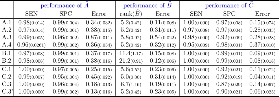
We use sensitivity (SEN), specificity (SPC) and relative error in Frobenius norm (Error) as criteria to evaluate the performance of the estimates of transition matricesA,B and C. Tuning parameters are chosen based on BIC. Since the exact contemporaneous dependence is not of primary concern, we omit the numerical results for Ωbu and Ωbv.
SEN = TP
TP + FN, SPE =
TN
FP + TN, Error =
|||Est.−Truth|||F |||Truth|||F .
Table 1: Model parameters under different model settings model parameters
p1 p2 rank(B∗) ρA ρC
model dimension
A.1 50 20 5 0.5 0.5
A.2 100 50 5 0.5 0.5
A.3 200 50 5 0.5 0.5
A.4 50 100 5 0.5 0.5
rank B.1B.2 100100 5050 1020 0.50.5 0.50.5
spectral radius
C.1 50 20 5 0.8 0.5
C.2 50 20 5 0.5 0.8
C.3 50 20 5 0.8 0.8
Table 2: Performance evaluation of Ab,Bb andCb under different model settings. performance of Ab performance ofBb performance ofCb
SEN SPC Error rank(Bb) Error SEN SPC Error
A.1 0.98(0.014) 0.99(0.004) 0.34(0.032) 5.2(0.42) 0.11(0.008) 1.00(0.000) 0.97(0.008) 0.15(0.074) A.2 0.97(0.014) 0.99(0.001) 0.38(0.015) 5.2(0.42) 0.31(0.011) 0.97(0.008) 0.97(0.004) 0.28(0.033) A.3 0.99(0.005) 0.96(0.002) 0.87(0.011) 5.8(0.92) 0.54(0.022) 0.98(0.000) 0.92(0.009) 0.28(0.028) A.4 0.96(0.0261) 0.99(0.002) 0.36(0.034) 5.2(0.42) 0.32(0.012) 0.95(0.009) 0.98(0.001) 0.37(0.010) B.1 0.97(0.008) 0.99(0.001) 0.37(0.017) 11.4(1.17) 0.15(0.008) 1.00(0.000) 0.99(0.001) 0.09(0.021) B.2 0.98(0.008) 0.99(0.001) 0.38(0.016) 21.2(0.91) 0.12(0.006) 1.00(0.000) 0.99(0.001) 0.08(0.018) C.1 1.00(0.000) 0.97(0.005) 0.25(0.015) 5.6(0.52) 0.23(0.006) 1.00(0.000) 0.92(0.021) 0.11(0.072) C.2 0.99(0.007) 0.95(0.004) 0.45(0.022) 5.0(0.00) 0.31(0.014) 1.00(0.000) 0.92(0.019) 0.04(0.011) C.3 1.00(0.000) 0.96(0.004) 0.18(0.013) 6.7(1.16) 0.19(0.011) 1.00(0.000) 0.87(0.029) 0.14(0.067) C.3’ 1.00(0.000) 0.99(0.002) 0.13(0.016) 5.2(0.42) 0.23(0.005) 1.00(0.000) 0.90(0.021) 0.06(0.023)
standard deviations are given in parentheses. Overall, the results are highly satisfactory and all the parameters are estimated with a high degree of accuracy. Further, all estimates were obtained in less than 20 iterations, thus indicating that the estimation procedure is numerically stable. As expected, when the the spectral radii of A and C increase thus leading to less stable {Xt} and {Zt} processes, a larger sample size is required for the estimation procedure to match the performance of the setting with same parameters but smaller ρ(A) and ρ(C). This is illustrated in row C.3’ of Table 2, where the sample size is increased to T = 500, which outperforms the results in row C.3 in whichT = 200 and broadly matches that of row A.1.
Since in some application settings the data may deviate from the posited Gaussian as-sumption, we further investigate the robustness of the algorithm in the presence of heavier than Gaussian distributions in the Supplementary Material??. Further, a brief comparison of the ML estimates with their two-step (non-iterative) counterparts is given in the Supple-mentary Material ??, that illustrates the numerical benefits of the proposed procedure.
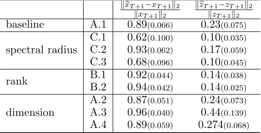
(L¨utkepohl, 2005). The performance metric is given by the relative error as measured by the`2norm of the out-of-sample pointsxT+1andzT+1, where the predicted values are given by bxT+1 =Axb T and zbT+1 =Bxb T +Czb T, respectively. It is worth noting that both {Xt} and {Zt}are mean-zero processes. However, since the transition matrix of {Xt} is subject to the spectral radius constraints to ensure the stability of the corresponding process, the magnitude of the realized value {xt} is small; whereas for {Zt}, since no constraints are imposed on theB coefficient matrix that encodes the inter-dependence,zt’s has the capac-ity of having relative large values in magnitude. Consequently, the relative error of bxT+1 is significantly larger than that of bzT+1, partially due to the small total magnitude of the denominator.
The results show that an increase in the spectral radius (keeping the other structural parameters fixed) leads to a decrease of the relative error, since future observations become more strongly correlated over time. On the other hand, an increase in dimension leads to a deterioration in forecasting, since the available sample size impacts the quality of the parameter estimates. Finally, an increase in the rank of the B matrix is beneficial for forecasting, since it plays a stronger role in the system’s temporal evolution.
Table 3: One-step-ahead relative forecasting error. kxbT+1−xT+1k2
kxT+1k2
kbzT+1−zT+1k2
kzT+1k2 baseline A.1 0.89(0.066) 0.23(0.075)
spectral radius
C.1 0.62(0.100) 0.10(0.035) C.2 0.93(0.062) 0.17(0.059) C.3 0.68(0.096) 0.10(0.045)
rank B.1 0.92(0.044) 0.14(0.038) B.2 0.94(0.042) 0.14(0.025)
dimension
A.2 0.87(0.051) 0.24(0.073) A.3 0.96(0.040) 0.44(0.139) A.4 0.89(0.059) 0.274(0.068)
5.2 Simulation results for the block Granger-causality test.
Next, we illustrate the empirical performance of the testing procedure introduced in Sec-tion4, together with the one specifically tailored to a sparse alternative (described in detail in the Supplementary Material??) with the null hypothesis beingB? = 0 and the alternative beingB? 6= 0, either low rank or sparse. Specifically, when the alternative hypothesis is true and has a low-rank structure, we use the general testing procedure proposed in Section 4, whereas when the alternative is true and sparse, we use the testing procedure presented in Supplementary Material ??. We focus on evaluating the type I error (empirical false rejection rate) when B?= 0, as well as the power of the test when B? has nonzero entries.
then further scaled down so that ρ(C?) = 0.5 or 0.8, depending on the simulation setting. Finally, we only consider the case where vtand uthave diagonal covariance matrices.
We use sub-sampling as in Politis et al. (1999) with the number of subsamples set to 3,000; an alternative would have been a block bootstrap procedure (e.g., Hall,1985). Note that the length of the subsamples varies across simulation settings in order to gain insight on how sample size impacts the type I error or the power of the test.
Low-rank testing. To evaluate the type I error control and the power of the test, we pri-marily consider the case where rank(B?) = 0, with the data alternatively generated based on rank(B?) = 1. We test the hypothesis H0: rank(B) = 0 and tabulate the empirical pro-portion of falsely rejectingH0 when rank(B∗) = 0 (type I error) and the probability that we rejectH0 when rank(B∗) = 1 (power). In addition, we also show how the testing procedure performs when the underlying B? has rank r ≥0. In particular, when rank(B?) =r?, the type I error of the test corresponds to the empirical proportion of rejections of the null hypothesisH0:r ≤r?, while the power of the test to the empirical proportion of rejections of the null hypothesis set to H0 : r ≤ (r?−1). The latter resembles the sequential test inJohansen(1988).
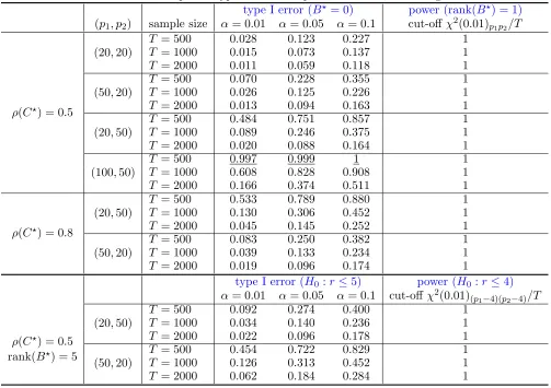
Empirically, we expect that whenB? = 0, the value of the proposed test statistic mostly falls below the cut-off value (upper α quantile), while when rank(B?) = 1, the value of the proposed test statistic mostly falls beyond the critical value χ2(α)p1p2/T with T being the sample size, hence leading to a detection. Table 4 gives the type I error of the test when setting α = 0.1,0.05,0.1, and the power of the test using the upper 0.01 quantile of the reference distribution as the cut-off, for different combinations of model dimensions (p1, p2) and sample size.
Based on the results shown in Table 4, it can be concluded that the proposed low-rank testing procedure accurately detects the presence of “Granger causality” across the two blocks, when the data have been generated based on a truly multi-layer VAR system. Further, when B? = 0, the type I error is close to the nominal α level for sufficiently large sample sizes, but deteriorates for increased model dimensions. In particular, relatively large values of p2 and larger spectral radiusρ(C?) negatively impact the empirical false rejection proportion, which deviates from the desired control level of the type I error. In the case where rank(B?) =r >0, the testing procedure provides satisfactory type I error control for larger sample sizes and excellent power.
Sparse testing. Since the rejection rule of the HC-statistic is based on empirical process theory (Shorack and Wellner, 2009) and its dependence on α is not explicit, we focus on illustrating how the empirical proportion of false rejections (type I error) varies with the sample size T, the model dimensions (p1, p2) and the spectral radius of C?. To show the power of the test, each entry in B? is nonzero with probability q ∈ (0,1) such that
Table 4: Empirical type I error and power for low-rank testing
type I error (B? = 0) power (rank(B?) = 1) (p1, p2) sample size α= 0.01 α= 0.05 α= 0.1 cut-offχ2(0.01)p1p2/T
ρ(C?) = 0.5
(20,20)
T = 500 0.028 0.123 0.227 1
T = 1000 0.015 0.073 0.137 1
T = 2000 0.011 0.059 0.118 1
(50,20)
T = 500 0.070 0.228 0.355 1
T = 1000 0.026 0.125 0.226 1
T = 2000 0.013 0.094 0.163 1
(20,50)
T = 500 0.484 0.751 0.857 1
T = 1000 0.089 0.246 0.375 1
T = 2000 0.020 0.088 0.164 1
(100,50)
T = 500 0.997 0.999 1 1
T = 1000 0.608 0.828 0.908 1
T = 2000 0.166 0.374 0.511 1
ρ(C?) = 0.8
(20,50)
T = 500 0.533 0.789 0.880 1
T = 1000 0.130 0.306 0.452 1
T = 2000 0.045 0.145 0.252 1
(50,20)
T = 500 0.083 0.250 0.382 1
T = 1000 0.039 0.133 0.234 1
T = 2000 0.019 0.096 0.174 1
type I error (H0:r ≤5) power (H0 :r≤4) α= 0.01 α= 0.05 α= 0.1 cut-offχ2(0.01)(p1−4)(p2−4)/T
ρ(C?) = 0.5 rank(B?) = 5
(20,50)
T = 500 0.092 0.274 0.400 1
T = 1000 0.034 0.140 0.236 1
T = 2000 0.022 0.096 0.178 1
(50,20)
T = 500 0.454 0.722 0.829 1
T = 1000 0.126 0.313 0.452 1
T = 2000 0.062 0.184 0.284 1
Table 5: Empirical type I error and power for sparse testing
type I error (B? = 0) power (SNR(B?) = 0.8) (p1, p2) 200 500 1000 2000 200 500 1000 2000
ρ(C?) = 0.5
(20,20) 0.244 0.097 0.074 0.055 1 1 1 1
(50,20) 0.393 0.131 0.108 0.074 1 1 1 1
(20,50) 0.996 0.351 0.153 0.093 1 1 1 1
(100,50) 1.000 0.963 0.270 0.115 1 1 1 1
ρ(C?) = 0.8 (50,20) 0.402 0.158 0.112 0.075 0.829 0.996 1 1
(20,50) 0.999 0.430 0.166 0.111 1 1 1 1
nonzero, empirically the test is always able detect its presence, as long as the effective signal-to-noise ratio is beyond the detection threshold.
6. Real Data Analysis Illustration.
We employ the developed framework and associated testing procedures to address one of the motivating applications. Specifically, we analyze the temporal dynamics of the log-returns of stocks with large market capitalization and key macroeconomic variables, as well as their cross-dependence. Specifically, using the notation in (1), we assume that the Xt block consists of the stock log-returns, while the macroeconomic variables form theZtblock. With this specification, we assume that the macroeconomic variables are “Granger-caused” by the stock market, but not vice versa. Note that our framework allows us to pose and test a more general question than previous work in the economics literature considered. For example, Farmer(2015) building on previous work byFitoussi et al. (2000); Phelps(1999) tests only the relationship between the employment index and the composite stock index, using a bivariate VAR model. On the other hand, our framework enables us to consider the components of the S&P 100 index and the “medium” list of macroeconomic variables considered in the work ofStock and Watson(2005).
Next, we provide a brief description of the data used. The stock data consist of monthly observations of 71 stocks corresponding to a stable set of historical components comprising the S&P 100 index for the 2001-2016 period. The macroeconomic variables are chosen from the “medium” list in Stock and Watson (2005). The complete lists of stocks and macroeconomic variables, together with the preprocessing to ensure stationarity used in this study are given in Supplementary Material ??.
We start the analysis by using the VAR model for the stock log-returns to study their evolution over the 2001-2016 period. Analogously to the strategy employed byBillio et al. (2012), we consider 36-month-long rolling-windows for fitting the modelXt=AXt−1+Ut, for a total of 143 estimates of the transition matrix A. VAR models involving more than 1 lag were also fitted to the data, but did not indicate temporal dependence beyond lag 1. To obtain the final estimates across all 143 subsamples, we employ stability selection
(Meinshausen and B¨uhlmann,2010), with the threshold set at 0.6 for including an edge in
A.1 Figure2depicts the global clustering coefficient (Luce and Perry,1949) of the skeleton of the estimated A over all 143 rolling windows, with the time stamps on the horizontal axis specifying the starting time of the corresponding window. The results clearly indicate strong connectivity in lead-lag stock relationships during the financial crisis period March 2007-June 2009. Next, we present the analysis based on the VAR-X component of our model, given by Zt = BXt−1+CZt−1 +Vt with the stock log-returns corresponding to the Xt block and the (stationary) macroeconomic variables to the Zt block. As before, we fit the data within each rolling window, with the tuning parameters based on a search over a 10×10 lattice (with (λB, λC) ∈ [0.5,4]×[0.2,2], equal-spaced) using the BIC. It should be noted that for the majority of the rolling windows, the rank of B is 1 (data not shown). The sparsity level of the estimated C over the 143 rolling windows is depicted in Figure 3. The connectivity patterns in C show more complex and nuanced patterns than
Figure 2: Global clustering coefficient of estimated Aover different periods
0.030.030.030.030.030.020.03 0.04
0.030.03 0.01
0.03 0.020.02
0.010.000.010.010.010.01 0.020.02
0.01 0.000.000.01
0.01 0.02 0.050.05 0.06 0.05 0.07
0.090.090.09
0.06 0.05
0.04 0.04
0.030.030.030.030.040.04 0.04
0.03 0.07
0.09 0.110.11
0.130.130.13 0.110.11
0.120.12 0.110.110.100.11
0.100.11 0.120.12
0.17 0.22
0.280.270.28 0.26 0.28 0.270.27 0.25 0.23 0.22 0.24 0.250.25 0.24 0.23 0.220.220.22
0.23 0.19 0.14 0.09 0.100.10 0.12 0.100.100.100.10
0.09
0.06 0.050.040.04
0.03 0.020.020.03
0.040.040.05 0.050.060.050.05
0.030.03 0.02
0.020.01 0.010.010.02
0.02 0.03
0.020.02 0.010.02
0.030.030.040.04 0.040.040.050.050.04
0.030.030.04 0.06 0 0.05 0.1 0.15 0.2 0.25 0.3
Sep-01 Mar-02 Sep-02 Mar-03 Sep-03 Mar-04 Sep-04 Mar-05 Sep-05 Mar-06 Sep-06 Mar-07 Sep-07 Mar-08 Sep-08 Mar-09 Sep-09 Mar-10 Sep-10 Mar-11 Sep-11 Mar-12 Sep-12 Mar-13 Global Clustering Coefficient of Estimated A
Figure 3: Sparsity of estimatedC over different periods
0.09 0.07 0.05 0.01 0.060.06 0.090.10 0.130.130.13
0.17 0.16 0.20 0.210.21 0.18 0.190.19 0.14 0.12 0.140.14 0.110.12 0.16 0.180.19 0.21
0.230.240.24
0.20 0.19 0.16 0.11 0.08 0.030.03 0.020.02 0.03 0.09
0.120.120.120.12 0.150.150.14
0.17 0.18 0.210.22 0.20 0.230.23 0.24 0.22 0.22 0.200.20 0.190.19
0.220.220.23 0.23
0.25 0.270.260.28
0.300.300.29 0.28
0.27 0.250.250.250.260.260.250.260.25
0.24 0.22 0.19 0.16 0.13 0.10 0.06 0.04
0.030.030.04 0.04 0.06 0.09 0.14 0.19 0.22 0.250.26 0.22 0.17 0.12 0.08 0.04
0.010.000.01 0.050.050.060.060.07
0.08
0.030.030.03 0.050.05 0.07 0.12 0.18 0.23 0.26 0.26 0.29 0.23
0.170.160.170.17
0 0.05 0.1 0.15 0.2 0.25 0.3 0.35
Jan-02 Jul-02 Jan-03 Jul-03 Jan-04 Jul-04 Jan-05 Jul-05 Jan-06 Jul-06 Jan-07 Jul-07 Jan-08 Jul-08 Jan-09 Jul-09 Jan-10 Jul-10 Jan-11 Jul-11 Jan-12 Jul-12 Jan-13
for stocks. A more detailed analysis of the various peaks identified through our model is given in Supplementary Material ??.
Based on the previous findings, we partition the time frame spanning 2001-2016 into the following periods: pre- (2001/07–2007/03), during- (2007/01–2009/12) and post-crisis (2010/01-2016/06) one. We estimate the model parameters using the data within the entire sub-period(s).
The estimation procedure of the transition matrix Afor different periods is identical to that described above using subsamples over rolling-windows. For the pre- and post- crisis periods, since we have 76 and 77 samples respectively, the stability selection threshold is set at 0.75, whereas for the during-crisis period, at 0.6 to compensate for the small sample size (36). Table6shows the average R-square for all 71 stocks, as well as its standard deviation, which is calculated based on in-sample fit; i.e.,the proportion of variation explained by using the VAR(1) model to fit the data. The overall sparsity level and the spectral radius of the estimated transition matrices A are also presented. The results are consistent with the previous finding of increased connectivity during the crisis. Further, for all periods the estimate of the spectral radius is fairly large, indicating strong temporal dependence of the log-returns.
Table 6: Summary for estimated Awithin different periods.
2001/07–2007/03 2007/01–2009/12 2010/01–2016/06
Averaged R sq 0.31 0.72 0.28
Sd of R sq 0.103 0.105 0.094
Sparsity level ofAb 0.17 0.23 0.19
Spectral radius ofAb 0.67 0.90 0.75
Next, we focus on the key motivation for developing the proposed modeling framework, namely the inter-dependence of stocks and macroeconomic variables over the specified three sub-periods. The p-value for testing the hypothesis of lack of block “Granger causality”
H0 : B = 0, together with the spectral radius and the sparsity level for the estimated
C transition matrices are listed in Table 7. Specifically, for all three periods, the rank of estimated B is 1, indicating that the stock market as captured by its leading stocks, “Granger-causes” the temporal evolution of the macroeconomic variables. The fact that the rank ofB is 1, indicates that the inter-block influence can be captured as a single portfolio acting in unison. To investigate the relative importance of each sector in the portfolio, we group the stocks by sectors. The proportion of each sector (up to normalization) is obtained by summing up the loadings (first right singular vector of the estimated B) of the stocks within this sector, weighted by their market capitalization (results shown in Supplementary Material??).
the analysis inFarmer(2015) is based on bivariate VAR models involving only employment and the stock index. Therefore, there is a possibility that the stock market is reacting to some other information captured by other macroeconomic variables, such as GDP, capital spending, inflation, interest rates, etc. However, our high-dimensional VAR model simulta-neously analyzes a key set of macroeconomic variables and also accounts for the influence of the largest stocks in the market. Hence, it automatically overcomes the criticism leveraged by Sims (1992) about misinterpretations of findings from small scale VAR models due to the omission of important variables, and further echoed in the discussion inBernanke et al. (2005). Other interesting findings are presented in Supplementary Material ??.
Table 7: Summary for estimated B and C within different periods.
2001/07–2007/03 2007/01–2009/12 2010/01–2016/16
p-value for testing H0 :B = 0 0.075 0.009 0.044
Sparsity level of Cb 0.06 0.25 0.06
Spectral radius ofCb 0.35 0.76 0.40
Table 8: Left Singular Vectors of Estimated B for different periods Pre-Crisis During-Crisis Post-Crisis
FFR -0.24 -0.26 -0.23
T10yr -0.09 0.14 0.16
UNEMPL -0.07 0.01 -0.07
IPI -0.43 0.34 0.26
ETTL 0.33 0.24 0.13
M1 0.23 -0.12 -0.47
AHES -0.01 0.30 0.17
CU -0.49 0.32 0.27
M2 0.10 -0.04 -0.32
HS 0.51 -0.02 -0.02
EX -0.18 0.41 0.06
PCEQI -0.07 -0.18 0.41
GDP 0.10 -0.02 0.05
PCEPI 0.00 0.14 -0.01
PPI -0.15 0.00 0.06
CPI 0.01 0.15 -0.31
SP.IND -0.06 -0.53 0.38
Remark 13 We also applied our multi-block model with the first block Xt corresponding
to the macro-economic variables and the second block Zt the stocks variables (results not