ISSN: 2231-5373
http://www.ijmttjournal.org
Page 277
Two Parameter Laplace Type Bimodal
Distribution
D V Ramana Murty*, G Arti** and M. VivekanandaMurty***
*Department of Statistics, VT College, Rajahmundry, East Godavari District, Andhra Pradesh, India. ** Department of Management, GITAM (Deemed to be University), Visakhapatnam, India.
and ***Former Professor of Statistics, Andhra University, Visakhapatnam, India.
Abstract
This paper is on the two parameter Laplace type Bimodal distribution. After discussing distributional properties, order statistics were developed and discussed. Inferential aspects were discussed and estimates of the parameters were obtained through Method of Moments and Maximum Likelihood Estimation techniques. Minimum unbiased estimator of the location parameter and best linear unbiased estimator of the location and scale parameter were also obtained.
Key words: Two parameter Laplace, Bimodal, Order statistics, Estimation of Parameters
I. INTRODUCTION
The Laplace distribution has received considerable attention as an appropriate model in reliability theory and life testing models.The statistical data in the fields like agriculture, meteorology and population studiesare appearing as if it is generated from a Laplace distribution, but have the kurtosis lies between 3 and 6. In this paper we introduce a two parameter Laplace type bimodal distribution which suits the distributionarising out of the situations mentioned above. The various distributional properties and inferential aspects of this distribution are discussed. This distribution can be viewed as a reflected gamma type distribution and a hybridization of Laplace and reflected two parameter gamma distribution.
II. TWO PARAMETER LAPLACE TYPE BIMODAL DISTRIBUTION
A continuous random variable 𝑋 is said to have a two parameter Laplace type bimodal distribution if its probability density function is of the form,
𝑓 𝑥, 𝜇, 𝛽 = 1 4𝛽
𝑥 − 𝜇 𝛽
2
𝑒− 𝑥−𝜇𝛽 , −∞< 𝑥 <∞, ∞< 𝜇 <∞, 𝛽 > 0 −→ 1
Making the transformations, 𝑦 =𝑥−𝜇𝛽 in equation (1), one can get
𝑓 𝑦 =14𝑦2𝑒− 𝑦 , −∞< 𝑥 <∞ −→ 2
which can be called as the standard Laplace type bimodal distribution. The various shapes of the frequency curves are shown in figure 1.
Case 1:𝜇 = 1, 𝛽 = 2
ISSN: 2231-5373
http://www.ijmttjournal.org
Page 278
Case 2:𝜇 = 1, 𝛽 = 1
Fig 1
Various shapes of theLaplace type bimodal distribution
III. PROPERTIES OF DISTRIBUTION
The distribution function is
𝐹𝑋(𝑥) = 1 4𝛽
𝑥 − 𝜇 𝛽
2
𝑒− 𝑥−𝜇𝛽 𝑑𝑥
𝑥
−∞
= 1 − 1 2+
𝑥 − 𝜇 𝛽 +
𝑥 − 𝜇 𝛽
2
𝑒− 𝑥−𝜇𝛽 , 𝑓𝑜𝑟 𝑥 ≥ 𝜇
= 12+ 𝑥−𝜇𝛽 + 𝑥−𝜇𝛽 2 𝑒− 𝑥−𝜇𝛽 , 𝑓𝑜𝑟 𝑥 < 𝜇3
Mean of the distribution is
𝐸 𝑋 = 𝑥𝑓 𝑥 𝑑𝑥 = 1 4𝛽 𝑥
𝑥 − 𝜇 𝛽
2
𝑒− 𝑥−𝜇𝛽 𝑑𝑥
∞
−∞ ∞
−∞
On simplification, one can have Mean= 𝜇
The Median ‘
M
’of this distribution is such that1 4𝛽 𝑥
𝑥 − 𝜇 𝛽
2
𝑒− 𝑥−𝜇𝛽 𝑑𝑥
𝑀
−∞
+ 1 4𝛽 𝑥
𝑥 − 𝜇 𝛽
2
𝑒− 𝑥−𝜇𝛽 𝑑𝑥
∞
𝑀
= 1
Solving this one can get Median = M= 𝜇. Hence the distribution is symmetric.
Taking the derivative of (1) with respect to
x
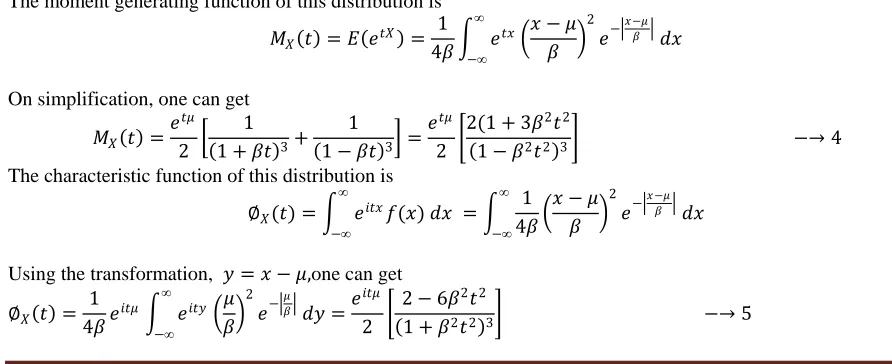
and equating to zero and solving for 𝑥, one can get the mode and, in this case,, the modes as 𝜇 − 2𝛽and𝜇 + 2𝛽. These two modes are separated by the distance of4𝛽. That is the distribution is Bimodal.The moment generating function of this distribution is
𝑀𝑋 𝑡 = 𝐸 𝑒𝑡𝑋 = 1 4𝛽 𝑒𝑡𝑥
𝑥 − 𝜇 𝛽
2
𝑒− 𝑥−𝜇𝛽 𝑑𝑥
∞
−∞
On simplification, one can get
𝑀𝑋 𝑡 = 𝑒𝑡𝜇
2 1 1 + 𝛽𝑡 3+
1 1 − 𝛽𝑡 3 =
𝑒𝑡𝜇 2
2(1 + 3𝛽2𝑡2
1 − 𝛽2𝑡2 3 −→ 4
The characteristic function of this distribution is
∅𝑋(𝑡) = 𝑒𝑖𝑡𝑥𝑓(𝑥) 𝑑𝑥 = 1 4𝛽
𝑥 − 𝜇 𝛽
2
𝑒− 𝑥−𝜇𝛽 𝑑𝑥
∞
−∞ ∞
−∞
Using the transformation, 𝑦 = 𝑥 − 𝜇,one can get
∅𝑋 𝑡 =4𝛽1 𝑒𝑖𝑡𝜇 𝑒𝑖𝑡𝑦 𝛽𝜇 2
𝑒− 𝜇𝛽 𝑑𝑦
∞
−∞
=𝑒 𝑖𝑡𝜇
2
2 − 6𝛽2𝑡2
1 + 𝛽2𝑡2 3 −→ 5
ISSN: 2231-5373
http://www.ijmttjournal.org
Page 279
To verify the additive property of the distribution,consider two independent Laplace type bimodal variables 𝑋1and 𝑋2with probability density function𝑓 𝑥1, 𝜇1, 𝛽1 and 𝑓 𝑥2, 𝜇2, 𝛽2 respectively and their characteristic functions
be∅𝑋1 𝑡 and∅2 𝑡 . For finding the distribution of 𝑋1+ 𝑋2 , one can obtain the characteristic function of𝑋1+ 𝑋2.
Since 𝑋1 and 𝑋2are independent,
∅𝑋1+𝑋2 𝑡 = ∅𝑋1 𝑡 ∅𝑋2 𝑡
Since
∅𝑋𝑗 𝑡 =𝑒
𝑖𝑡 𝜇 𝑗
2 1 1+𝑖𝛽𝑗𝑡 3+
1
1−𝑖𝛽𝑗𝑡 3 , j =1,2
then
∅𝑋1+𝑋2 𝑡 =
𝑒𝑖𝑡(𝜇1+𝜇2) 2
1 1 + 𝑖𝛽1𝑡 3+
1
1 − 𝑖𝛽1𝑡 3 + 1 1 + 𝑖𝛽2𝑡 3+
1
1 − 𝑖𝛽2𝑡 3 −→ 6
Since (6) is not in the form of (5) one can say that the distribution of 𝑋1+ 𝑋2is not a Laplace type bimodal
distribution. Hence the additive property does not hold good for this distribution. The central moments of this distribution are
𝜇2𝑛 = 1
4𝛽 𝑥 − 𝜇 2𝑛 𝑥 − 𝜇
𝛽 2
𝑒− 𝑥−𝜇𝛽 𝑑𝑥
∞
−∞
Making the necessary transformation and by integration, one can get
𝜇2𝑛=
2𝑛 + 2 ! 𝛽2𝑛
2 𝑎𝑛𝑑 𝜇2𝑛+1 = 0 −→ 7
Further, the first four central moments of this distribution are
𝜇1= 0, Variance= 𝜇2= 12𝛽2, 𝜇3= 0, 𝜇4= 360𝛽4
Since, the distribution is symmetric, its skewness is zero.
The kurtosis of this distribution is
𝛽2= 𝜇4 𝜇22=
360𝛽4
12𝛽2 = 2.5 < 3
Hence the distribution is platykurtic having the peak less than the Laplace distribution.
The recurrence relation between the central moments is obtained as
𝜇2𝑛 =
(2𝑛 + 1) 2𝑛 + 2
2𝑛(2𝑛 − 1) 𝛽2𝜇2𝑛−2 −→ 8
The 𝑝𝑡 order absolute moments of the distribution are
𝐸 𝑋 − 𝜇 𝑝 = 1
4𝛽 𝑥 − 𝜇 𝑝 𝑥 − 𝜇
𝛽 2
𝑒− 𝑥−𝜇𝛽 𝑑𝑥
∞
−∞
On simplification, one can have
𝐸 𝑋 − 𝜇 𝑝 = 𝑝 + 2 !
2 𝛽𝑝 −→ 9
The Mean deviation about mean𝜇 of the distribution is𝑀 𝐷 = 3𝛽 The ratio of the mean deviation to standard deviation is 3𝛽
12𝛽 = 0.866
The distribution of the square of the variate 𝑌 = 𝑋2 can be obtained as
𝑓 𝑦 = 1 4𝛽 𝑦
𝑦 𝛽
2
𝑒− 𝑦𝛽 , 0 ≤ 𝑦 <∞
For obtaining the sampling distribution, assume𝜇 = 0 without loss of generality. Let 𝑥1, 𝑥2, … . 𝑥𝑛 bea sample drawn
ISSN: 2231-5373
http://www.ijmttjournal.org
Page 280
𝑓 𝑥 = 1 4𝛽
𝑥 𝛽
2
𝑒− 𝑥 𝛽 , −∞< 𝑥 <∞ −→ 10
The sample observations 𝑥1, 𝑥2, … . 𝑥𝑛are independently identically distributed as given in (10).
Since𝑥1, 𝑥2, … . 𝑥𝑛 are independently distributed, the characteristic function of𝑥1, 𝑥2, … . 𝑥𝑛 is given by
∅ 𝑡 = 1
4𝛽 𝑒𝑖𝑡 𝑥 𝑥 𝛽
2 𝑒− 𝑥 𝛽
∞
−∞
𝑑𝑥 −→ 11
If 𝑢 = 𝑛𝑖=0𝑥𝑖 then the distribution function of, namely 𝑝 𝑢 , is given by
𝑝 𝑢 = 1
2𝜋 𝑒𝑖𝑡𝑢 1
4𝛽 𝑒𝑖𝑡 𝑥 𝑥 𝛽
2 𝑒− 𝑥 𝛽
∞
−∞
𝑑𝑥 𝑛
∞
−∞
𝑑𝑢 −→ 12
On simplification
𝑝 𝑢 = 1 2𝜋
1
2𝑛𝛽𝑛 𝑒𝑖𝑡𝑢 1
1 − 𝑖𝛽𝑡 3𝑛𝑑𝑢 −→ 13
∞
−∞
The poles of the integrand are of the 3nth order and one of those is 1 − 𝑖𝛽𝑡 3𝑛. From the well-known residue theorem of Cauchy Macro Bert (1933), one can have
𝑝 𝑢 = 1 2𝑛𝛽𝑛
1 𝑖3𝑛−1
𝑑3𝑛−1 𝑑𝑡3𝑛−1
𝑒−𝑖𝜇𝑡
1−𝑖𝛽𝑡 3𝑛 𝑡
𝑡=1
𝛽 𝑖
−→ 14
The distribution of arithmetic mean of the sample mean of the sample size
n
is𝑝 𝑥 = 𝑛 3𝑛𝛽𝑛
−1 𝑛+2𝑗 −1 𝑛 + 2𝑗 − 𝑖 ! 𝑛
𝑗 =1
1 𝑖(𝑛 + 2𝑗 − 1)
𝑑𝑛+2𝑗 −1 𝑑𝑡𝑛+2𝑗 −1
𝑒−𝑖𝑡𝑛 𝑥 1+𝑖𝛽𝑡 𝑛 +2𝑗
𝑡
𝑡=1
𝛽 𝑖
−→ 15
defined for all values of on the range(−∞< 𝑥 <∞).
IV. ORDER STATISTICS OF TWO PARAMETER LAPLACE TYPE BIMODAL DISTRIBUTION
The simple explicit form of the distribution function as given in (3) leads to derive the order statistics connected with this two parameter Laplace type bimodal distribution. For simplicity, let us assume 𝜇 = 0, 𝛽 = 1 then the probability density function (1) reduces to
𝑓 𝑥 =1
4𝑥2𝑒− 𝑥 , −∞< 𝑥 <∞ −→ 16
Let 𝑋1:𝑛 ≤ 𝑋2:𝑛≤ ⋯ 𝑋𝑛:𝑛denote the order statistics obtained from a random sample of size ‘n’ from the standardized
Laplace distribution having the probability density function of the form given in (1). The probability density function of the mth order statistics is given by [David (1991)].
𝑓𝑚:𝑛 𝑥 = 𝐷𝑚:𝑛 𝑓 𝑥 𝑚−1 1 − 𝐹 𝑥 𝑛−𝑚𝑓 𝑥 , −∞< 𝑥 <∞
where
𝐷𝑚:𝑛=
𝑛!
𝑚 − 1 ! 𝑛 − 𝑚 ! −→ 17
Substituting 𝐹 𝑥 values in the above equation (17), one can get
𝑓𝑚:𝑛 𝑥 = 𝐷𝑚:𝑛 1
4𝑥2𝑒− 𝑥 𝑛 − 𝑚
𝑞 𝑛−𝑚
𝑞=0
(−1)𝑞 1 − 𝑙
𝑘 2𝑘 ! 𝑥𝑖
𝑖!𝑒− 𝑥 2𝑘
𝑖=0 𝑙
𝑘=0
𝑚+𝑞−1
𝑓𝑜𝑟 𝑥 ≥ 0
𝑓𝑚:𝑛 𝑥 = 𝐷𝑚:𝑛14𝑥2𝑒− 𝑥 𝑛 − 𝑚𝑞 𝑛−𝑚
𝑞=0
(−1)𝑞 𝑙𝑘 2𝑘 ! 𝑥𝑖
𝑖!𝑒 − 𝑥 2𝑘 𝑖=0 𝑙
𝑘=0
4
𝑚+𝑞−1
𝑓𝑜𝑟 𝑥 < 0
(18)
where, 𝐷𝑚:𝑛 is as given in (17).
The
a
thISSN: 2231-5373
http://www.ijmttjournal.org
Page 281
𝛼𝑚:𝑛 𝑥 =
(−𝑥)∞ 𝑎
0 𝐷𝑚:𝑛𝑥2𝑒−𝑥
𝑛 − 𝑚 𝑞 𝑛−𝑚
𝑞=0 (−1)𝑞
𝑙𝑘 2𝑘 ! 2𝑘𝑖=0𝑥𝑖𝑖!𝑒− 𝑥
𝑙 𝑘=0
4
𝑚+𝑞−1
𝑑𝑥 +
(𝑥)𝑎 𝑎
0 𝐷𝑚:𝑛𝑥2𝑒−𝑥
𝑛 − 𝑚 𝑞 𝑛−𝑚
𝑞=0 (−1)𝑞 1 −
𝑙𝑘 2𝑘 ! 2𝑘𝑖=0𝑥𝑖𝑖!𝑒− 𝑥
𝑙 𝑘=0
4
𝑚+𝑞−1
𝑑𝑥 19
Define 𝐷𝑚:𝑛=𝐷𝑚 :𝑛4 and after simplifying 𝛼𝑚:𝑛 𝑎
= (−1)𝑎𝐷
𝑚:𝑛 𝑙𝑘 𝑙 𝑝=0 𝑗 𝑙=0 𝑚+𝑞−1 𝑗 =0 𝑛−𝑚 𝑞=0 𝑙 𝑘=0
𝑛 − 𝑚
𝑞 𝑚 + 𝑞 − 1𝑗 𝑗𝑙 𝑙
𝑝 2𝑗 −1+𝑙−𝑝(−1)𝑞
𝑎 + 2𝑘 + 𝑙 + 𝑝 ! (𝑚 + 𝑞)𝑎+2𝑘+𝑙+𝑝+1
+𝐷𝑚:𝑛 𝑙𝑘 𝑙 𝑝=0 𝑗 𝑙=0 𝑚+𝑞−1 𝑗 =0 𝑛−𝑚 𝑞=0 𝑙 𝑘=0
𝑛 − 𝑚
𝑞 𝑚 + 𝑞 − 1𝑗 𝑗𝑙 𝑙 𝑝 2𝑗𝑙 −𝑝
𝑎 + 2𝑘 + 𝑖 + 𝑝 ! (1 + 𝑙)𝑎+2𝑘+𝑖+𝑝+𝑙 → 20
Probability distribution of first ordered statistics is
𝑓1:𝑛 𝑥 =𝑛4𝑥2𝑒−𝑥 𝑛 − 1𝑞 (−1)𝑞 𝑛−1
𝑞=0
1 − 𝑙𝑘 2𝑘 ! 2𝑘 𝑥𝑖!𝑖𝑒−𝑥 𝑖=0 𝑙
𝑘=0 4
𝑞
𝑓𝑜𝑟 𝑥 ≥ 0
𝑓1:𝑛 𝑥 = 𝑛
4𝑥2𝑒− 𝑥 𝑛 − 1
𝑞 (−1)𝑞 𝑛−1
𝑞=0
𝑙𝑘 2𝑘 ! 2𝑘 𝑥𝑖!𝑖𝑒− 𝑥 𝑖=0 𝑙
𝑘=0
4
𝑞
𝑓𝑜𝑟 𝑥 < 0 −→ 21
The expected value of the first order statistics is
𝐸 𝑋(1) = 𝑛 − 𝑙𝑘 𝑙 𝑝=0 𝑗 𝑙=0 𝑚+𝑞−1 𝑗 =0 𝑛−𝑚 𝑞=0 𝑙 𝑘=0
𝑛 − 1 𝑞
𝑞
𝑗 𝑗𝑙 𝑝 2𝑙 𝑙−𝑝
𝑎 + 2𝑘 + 1 + 𝑝 ! (1 + 𝑞)𝑎+2𝑘+𝑖+𝑝+𝑙+1
+ 𝑙𝑘 𝑖 𝑝=0 𝑙 𝑖=0 𝑚+𝑞−1 𝑙=0 𝑛−1 𝑞=0 𝑙 𝑘=0
𝑛 − 1
𝑞 𝑞𝑙 𝑙𝑖 𝑖 𝑝 2𝑙−𝑝
𝑎 + 2𝑘 + 𝑖 + 𝑝 !
(1 + 𝑙)𝑎+2𝑘+𝑖+𝑝+𝑙 −→ 22
The
n
th order statistics of the distribution is same as the first order statistic with negative variate because the distribution is symmetric.A. Distribution of the Median
To obtain the distribution of the median, substitute 𝑚 =𝑛+12 if
n
is odd in (17). Then one can get𝑓𝑛 +1
2 :𝑛 𝑥 = 𝐷 𝑛 +1
2 :𝑛 1
4𝑥2𝑒− 𝑥 𝑛 − 1
2 𝑞 𝑛 −1
2
𝑞=0
−1 𝑞 1 − 𝑙𝑘 2𝑘 ! 𝑥𝑖 𝑖!𝑒 − 𝑥 2𝑘 𝑖=0 𝑙 𝑘=0 4 𝑛 +2𝑞−1 2 ,
𝑓𝑜𝑟 𝑥 ≥ 0
= 𝐷𝑛 +1 2 :𝑛
1
4𝑥2𝑒− 𝑥 𝑛 − 1
2 𝑞 𝑛 −1
2
𝑞=0
−1 𝑞 𝑙𝑘 2𝑘 ! 𝑥𝑖 𝑖!𝑒 − 𝑥 2𝑘 𝑖=0 𝑙 𝑘=0 4 𝑛 +2𝑞−1 2
𝑓𝑜𝑟 𝑥 < 0−→ 23
Where,𝐷𝑛 +1 2 :𝑛=
𝑛!
𝑛 −12 ! 2
ISSN: 2231-5373
http://www.ijmttjournal.org
Page 282
𝑓2𝑛 +1
4 :𝑛 𝑥 = 𝐷 2𝑛 +1
4 :𝑛 1
4𝑥2𝑒− 𝑥 2𝑛 − 1
4 𝑞 2𝑛 −1
4
𝑞=0
−1 𝑞 1 − 𝑙𝑘 2𝑘 ! 𝑥𝑖
𝑖!𝑒 − 𝑥 2𝑘
𝑖=0 𝑙
𝑘=0 4
2𝑛 +2𝑞−1 4
for 𝑥 ≥ 0
= 𝐷2𝑛 +1 4 :𝑛
1
4𝑥2𝑒− 𝑥 2𝑛 − 1
4 𝑞 2𝑛 −1
4
𝑞=0
−1 𝑞 𝑙𝑘 2𝑘 ! 𝑥𝑖
𝑖!𝑒 − 𝑥 2𝑘
𝑖=0 𝑙
𝑘=0
4
2𝑛 +4𝑞−3 3
for 𝑥 < 024 Where 𝐷2𝑛 +1
4 :𝑛=
𝑛!
2𝑛 −34 ! 2
B. Joint Moments of the Order Statistics
The joint probability density function of the𝑚𝑡 and 𝑠𝑡 order statistics𝑋𝑚:𝑛and𝑋𝑠:𝑛, 𝑚 < 𝑠 is given by
[David (1981)]
𝑓𝑚,𝑠:𝑛 𝑥 = 𝐷𝑚,𝑠:𝑛 𝐹 𝑥 𝑚−1 𝐹 𝑦 − 𝐹 𝑥 𝑠−𝑚−1 1 − 𝐹 𝑦 𝑛−𝑠𝑓 𝑥 𝑓(𝑦)
Where 𝐷𝑚,𝑠:𝑛 = 𝑚−1 ! 𝑠−𝑚−1 ! 𝑛−𝑠 !𝑛!
And𝐹 𝑥 is the cumulative density function of the laplace type distribution as given in equation (3)
Writing 𝑥 =2+2𝑥+𝑥4 2, it is possible to express the joint density function of 𝑋𝑚:𝑛and𝑋𝑠:𝑛 as 𝑓𝑚,𝑠:𝑛 𝑥 = 𝐷𝑚,𝑠:𝑛 𝑈 𝑥 𝑚−1 𝑈 𝑦 − 𝑈 𝑥 𝑠−𝑚−1 1 − 𝑈 𝑦 𝑛−𝑠𝑓 𝑥 𝑓 𝑦 → 25
where 𝐷𝑚,𝑠:𝑛 = 𝑚−1 ! 𝑠−𝑚−1 ! 𝑛−𝑠 !𝑛! 𝑓𝑜𝑟 𝑥, 𝑦 : −∞< 𝑥 < 𝑦 <∞
This region can be split into three mutually exclusive regions,
𝑅1: 𝑥, 𝑦 : −∞< 𝑥 < 𝑦 < 0 𝑅2: 𝑥, 𝑦 : 0 < 𝑥 < 𝑦 <∞
𝑅3: 𝑥, 𝑦 : −∞< 𝑥 <∞, −∞< 𝑦 <∞
With this splitting of the region of the product moments can be obtained as
𝐸[𝑋𝑚:𝑛, 𝑋𝑠:𝑛] =
𝐷𝑚,𝑠:𝑛 𝑥𝑦 𝑈 −𝑥 𝑚−1 𝑈 −𝑦 − 𝑈 −𝑥 𝑠−𝑚−1 1 − 𝑈 −𝑦 𝑛−𝑠𝑓 −𝑥 𝑓 −𝑦 𝑑𝑥𝑑𝑦 𝑅1
+𝐷𝑚,𝑠:𝑛 𝑥𝑦 1 − 𝑈 𝑥 𝑚−1 𝑈 𝑥 − 𝑈 𝑦 𝑠−𝑚−1 1 − 𝑈 𝑦 𝑚−𝑠𝑓 𝑥 𝑓 𝑦 𝑑𝑥𝑑𝑦 𝑅2
−𝐷𝑚,𝑠:𝑛 (−𝑥𝑦) 𝑈 𝑥 𝑚−1 1 − 𝑈 −𝑥 − 𝑈 −𝑦 𝑠−𝑚−1 𝑈 𝑦 𝑛−𝑠𝑓 𝑥 𝑓 𝑦 𝑑𝑥𝑑𝑦 𝑅3
→ 26
Expanding the binomial expression in the integral, one can have
𝐸[𝑋𝑚:𝑛, 𝑋𝑠:𝑛] = 𝐷𝑚,𝑠:𝑛 𝑠 − 𝑚 − 1𝑖 𝑛 − 𝑠
𝑗 𝑛−𝑠
𝑗 =0 𝑠−𝑚−1
𝑖=0
−1 𝑠−𝑚−1+𝑖+𝑗Ψ(𝑠 − 2 − 𝑖, 𝑖 + 𝑗)
+𝐷𝑚,𝑠:𝑛 𝑠 − 𝑚 − 1𝑗 𝑚 − 1𝑗 𝑠−𝑚−1
𝑗 =0 𝑚−1
𝑖=0
−1 𝑖+𝑗Ψ(𝑠 − 𝑚 − 1 + 𝑖 + 𝑗, 𝑛 − 𝑠 + 𝑗)
−𝐷𝑚,𝑠:𝑛 𝑠 − 𝑚 − 1𝑗 𝑠 − 𝑚 − 1 − 𝑖𝑖 𝑛−𝑠
𝑗 =0 𝑠−𝑚−1
𝑖=0
−1 𝑖+𝑗 𝑥 𝑈 𝑥 𝑚+𝑖−1𝑓 𝑥 𝑑𝑥 𝑦 𝑈 𝑦 ∞ 𝑛−𝑠−𝑗𝑓 𝑦 𝑑𝑦 0
𝑥
0
ISSN: 2231-5373
http://www.ijmttjournal.org
Page 283
and Ψ 𝑎, 𝑏 = 𝑥𝑦 𝑈 𝑥 0∞ 0𝑦 𝑎 𝑈 𝑦 𝑏𝑓 𝑥 𝑓 𝑦 𝑑𝑥𝑑𝑦 −→ 27
Ψ 𝑎, 𝑏 = 𝑥𝑦 𝑙𝑘 2𝑘 ! 𝑥𝑖
𝑖!𝑒 − 𝑥 2𝑘
𝑖=0 𝑙
𝑘=0
4
𝑎 𝑦
0
∞
0 𝑙𝑘 2𝑘 !
𝑦𝑖 𝑖!𝑒− 𝑥 2𝑘
𝑖=0 𝑙
𝑘=0
𝑏 2 + 𝑥2
4 𝑒−𝑥
2 + 𝑦2
4 𝑒−𝑦𝑑𝑥𝑑𝑦
= 1
4𝑎+𝑏+2 𝑙𝑘 𝑎 𝑟
𝑟
𝑗 𝑗𝑖 2𝑟−𝑖 𝑗
𝑖=0 𝑟
𝑗 =0 𝑎
𝑗 =0 𝑙
𝑘=0
Γ(2𝑘 + 𝑗 + 𝑖 + 2) (𝑟 + 1)(2𝑘 + 𝑗 + 𝑖 + 3)
− (𝑟 + 1)
𝑗1
𝑗! 2𝑘+𝑗 +𝑖+2
𝑗1
Γ(2𝑘 + 𝑗 + 𝑗1+ 𝑖 + 2
2(𝑟 + 1) 2𝑘+𝑗 +𝑗1+𝑖+3 −→ 28
Substituting the value of Ψ 𝑎, 𝑏 of (28) in (20), one can get the moments of the order statistics.
V. INFERENTIAL ASPECTS OF THE TWO PARAMETER LAPLACE TYPE BIMODAL DISTRIBUTION
In the earlier section the two parameter Laplace type bimodal distribution was studied its distributional properties were presented. Another aspect of any distributional study is to look into the inferential aspects of the distribution, in particular the estimation of the parameters involved in the distribution under study. In this section various methods of estimation using the method of moments, maximum likelihood method estimation and best linear unbiased estimation in estimating the parameters of the two parameter Laplace type bimodal distribution were discussed. The asymptotic behaviors of these estimators are also studied.
A. Method of moments
Let us consider a sample of size ‘n’ drawn from a population having the probability density function of the form given by
𝑓 𝑥, 𝜇, 𝛽 = 1 4𝛽
𝑥 − 𝜇 𝛽
2
𝑒− 𝑥−𝜇𝛽 , −∞< 𝑥 <∞, −∞< 𝜇 <∞, 𝛽 > 0
This distribution is having two parameters 𝜇 and 𝛽. Hence, we consider the first two moments of the sample and the population, which leads to the following equations.
𝜇 = 𝑥, 12 𝛽2= 𝑠2=1
𝑛 𝑥𝑖− 𝑥 2 𝑛
𝑖=1
These equations give us the moment estimators as
𝜇 = 𝑥 𝑎𝑛𝑑 𝛽 2= 𝑠2
12= 0.0833𝑠2 −→ 29
The variance of 𝜇 is
𝑉𝑎𝑟 𝑥 = 𝑉𝑎𝑟 1 𝑛 𝑥𝑖
𝑛
𝑖=1
= 1
𝑛2 𝑉𝑎𝑟 𝑥𝑖 = 1
𝑛2 12𝛽2 −→ 30 𝑛
𝑖=1
and 𝐸 𝑥 = 𝐸 𝑛1 𝑛𝑖=1𝑥𝑖 =1𝑛 𝑛𝑖=1𝐸(𝑥𝑖) = 𝜇
Therefore, the sample mean is an unbiased estimator of𝜇. For obtaining the unbiased estimator of𝛽2, consider
𝛽 ∗2= 𝑛
𝑛 − 1 0.0833 𝑠2 𝐸(𝛽 ∗2) = 𝛽2
Therefore, 𝛽 ∗2is an unbiased estimator of 𝛽2. The variance of 𝛽 ∗2can be obtained as
𝑉𝑎𝑟 𝛽 ∗2 = 𝑉𝑎𝑟 𝑛
𝑛 − 1 0.0833 𝑠2 = 𝑛2
ISSN: 2231-5373
http://www.ijmttjournal.org
Page 284
Where 𝑉𝑎𝑟 𝑠2 =𝜇4−𝜇2 2
𝑛 −
2 𝜇4−𝜇22
𝑛2 +
𝜇4−3𝜇22
𝑛3 and 𝜇𝑖is the 𝑖𝑡 central moment (Cramer,1946)
Therefore,
𝑉𝑎𝑟 𝑠2 = 360 − 144 𝛽4
𝑛 −
2 360 − 288 𝛽4
𝑛2 +
360 − 432 𝛽4
𝑛3 =
216 𝑛 −
144 𝑛2 −
72
𝑛3 𝛽4 −→ 33
Equations (32) and (33) gives
𝑉𝑎𝑟 𝛽 ∗2 = 𝑛2 𝑛 − 1 2
216 𝑛 −
144 𝑛2 −
72
𝑛3 0.0833 2 𝛽4 −→ 34
From the equations (32) and (34) it can be observed that as 𝑛 →∞ the variances tend to zero. Hencethe estimators𝑥 and𝛽 ∗2are consistent. Since the sample observations are independently distributed, these estimators are strongly consistent. Since the covariance of 𝑥 and𝛽 ∗2 is zero,these estimators 𝑥 and𝛽 ∗2 are uncorrelated. This result can also be visualized from the fact that the sample is drawn from a symmetric distribution.
B. Maximum Likelihood Method of Estimation
Let 𝑥1, 𝑥2, … . 𝑥𝑛 be a sample of size n drawn from a population having the probability density function of the
form given in equation (1). Then the likelihood function of the sample is
𝐿 = 4𝛽 1 𝑛𝜋𝑖=1𝑛 𝑥𝑖− 𝜇
𝛽 2
𝑒− 𝑛𝑖=1𝑥𝑖−𝜇𝛽 −→ 35
Taking logarithms on both sides of (35) gives
𝑙𝑜𝑔𝐿 = −𝑛𝑙𝑜𝑔 4𝛽 + 𝑙𝑜𝑔 𝑥𝑖− 𝜇 𝛽
2 − 𝑛
𝑖=1
𝑥𝑖− 𝜇 𝛽 𝑛
𝑖=1
−→ 36
For obtaining the maximum likelihood estimators of the parameters one has tomaximize L or
log
L
with respect to the parameters 𝜇 and𝛽. Sinceequation (32) is not differentiable with respect to𝜇the likelihood estimator of𝜇can be obtained as follows.Since the density function is symmetric about 𝑥 = 𝜇i.e𝑓 𝑥 + 𝜇 = 𝑓(𝑥 − 𝜇)it follows that𝐸(𝑥) = 𝜇. Hence𝑛1 𝑛𝑖=1 𝑥𝑖− 𝜇 is the mean deviationof the random sample from its mean. This shall be minimum if is the
median of the sample. Since
𝑀𝑎𝑥 𝑙𝑜𝑔𝐿 = 𝑀𝑎𝑥 𝑙𝑜𝑔 𝑥𝑖− 𝜇 𝛽
2 − 𝑛
𝑖=1
𝑥𝑖− 𝜇 𝛽 𝑛
𝑖=1
= 𝑀𝑖𝑛 𝑥𝑖− 𝜇 𝑛
𝑖=1
it can be shown that 𝜇 = Median of the sample if n is odd. If n is even, then 𝑋𝑛
2−1 ≤ 𝜇 ≤ 𝑋𝑛2+1.where 𝑋𝑗 is the𝑗
𝑡 order statistic.
After obtaining the maximum likelihood estimation of𝜇 as𝜇 and substituting𝜇 in equation (32) the maximum likelihood estimation of 𝛽2 can be obtained by differentiating log L with respect to 𝛽2 and equating it to zero.After simplification one can obtain
𝛽 =2 −𝑛+ 𝑛𝑖=1 𝑥𝑖−𝜇
2𝑛 .
Also, since 𝐸 −𝜕𝜕 𝛽2𝑙𝑜𝑔𝐿2 2
−1
= 𝐸 2𝛽𝑛4+12 𝑛𝑖=1 𝑥𝑖−𝜇
𝛽4
−1 = 2𝛽𝑛4
The approximate expression to the asymptotic variance of 𝛽2can be obtained as
𝐴𝑠𝑦𝑣𝑎𝑟 𝛽 = 𝐸 2 −𝜕 2𝑙𝑜𝑔𝐿
𝜕 𝛽2 2 −1
= 2𝛽 4
𝑛
C. Minimum variance unbiased estimators
ISSN: 2231-5373
http://www.ijmttjournal.org
Page 285
sample and to determine the linear coefficients 𝑙1, 𝑙2, … 𝑙𝑛so that the estimator is unbiased and minimum variance in
this class of estimators. [C.R.Rao (1974)]. Here note that the random sample here means a set of i. i. d random variables.
The condition of unbiasedness leads to𝑙1+ 𝑙2+ ⋯ + 𝑙𝑛 = 𝑙and the condition of minimum variance leads to𝑙12+ 𝑙22+ ⋯ + 𝑙𝑛2being minimum.
Writing,𝑙 =𝑙1+𝑙2+⋯+𝑙𝑛 𝑛one can have 𝑙𝑖− 𝑙 2
≥ 0 𝑛
𝑖=1
and this implies, 𝑛𝑖=1𝑙𝑖2≥ 𝑛𝑙 2=1𝑛, since 𝑛𝑖=1𝑙𝑖 = 1
Equality occurs only when all the𝑙𝑖 ’s are equal.ie. 𝑙𝑖 =1𝑛
Thus, the greatest lower bound of 𝑛𝑖=1𝑙𝑖2for various𝑙is 1
𝑛and is attained.
Therefore,𝜇 = 𝑥 , is the minimum variance unbiased estimator. The same holds for any value of𝜇. Hence it is also uniformly minimum variance unbiased estimator.
The minimum variance in this case is 𝑣𝑎𝑟 𝑥 𝑛 =12𝛽𝑛2
For obtaining the minimum variance unbiased estimator of𝛽2, consider the usual estimator 𝛽∗2which is unbiased. It can also be observed that it is the minimum variance unbiased estimator of 𝛽2
D. Best Linear Unbiased Estimators
Following the heuristic argument of Govindarajalu(1966) the best linear unbiased estimators of the location and scale parameters involved in the two parameter Laplace type bimodal distribution having the probability density function of the form given in (1) are obtained as follows.
Then the best linear unbiased estimators of𝜇 and 𝛽are given by Lloyd (1952) as
𝜇∗=𝑙′Ω𝑋
𝑙′Ω𝑙 𝑎𝑛𝑑 𝛽∗=
𝛼′Ω𝑋
𝛼′Ωα
where 𝑙′= 1,1, … ,1 , 𝑋′= 𝑋1:𝑛, 𝑋2:𝑛, … 𝑋𝑛:𝑛 𝑎𝑛𝑑 𝛼′= 𝛼1:𝑛, 𝛼2:𝑛, … 𝛼𝑛:𝑛
and𝛼1:𝑛 is the first moment of the𝑖𝑡 order statistics and Ω is the variance matrix of vector
X
The variance of these estimators are
𝑣𝑎𝑟(𝜇∗) =12𝛽2
𝑙′Ω𝑙 , 𝑣𝑎𝑟 𝛽∗ =
12𝛽 2 𝛼′Ωα
Where Ω is the standard deviation of the populationand 𝑐𝑜𝑣(𝜇∗, 𝛽∗) = 0. With the moments of the order statistics given in section (2.4) one can compute 𝜇∗and𝛽∗ and their variances respectively.
VI. CONCLUSIONS
This paper is on the distributional properties of the two parameter Laplace type bimodal distribution. The order statistic was also studies. In addition, inferential aspects like estimation of the parameters by method of moments, Maximum likelihood method of estimation were explained. Minimum variance unbiased estimators and Best linear unbiased estimators for the parameters of the distribution were presented.
REFERENCES
[1] Cramer, H. (1946): Mathematical Methods of Statistics, Asia Publishing House. [2] David. H.A. (1981): Order Statistics, John Wiley & Sons, Ins. New York
[3] Eisenberger, I. (1964): ‘Genesis of Bimodal distributions’ techno metrics, p.357-363., vol.6.
[4] Feller, W. (1966). An Introduction to Probability Theory and Its Applications, Vol.II, New York, John Wiley & sons, NC. [5] Govindarajulu, Z. (1966): Best linear estimates under symmetric censoring of the parameters of a double exponential population, [6] Johnson, N.L. and Kotz, S. (1970): Continuous Univariate Distributions, john Wiley Sons, New York.
[7] Kameda, T. (1928): On the reduction of frequency curves, SckandinaviskAktuarietidskrift, 11.
[8] Laplace, P.S. (1774): Memoire sur la pobabilite des causes par les evenemens, Memoiries de mathematique et de Physique, 6. [9] Lloyd, E.H. (1952): Least square estimation of location and scale parameters using order statistics, Biometrica, 39