A novel method for expediting the development of patient-reported outcome measures and an evaluation of its performance via simulation

R E S E A R C H A R T I C L E

Open Access

A novel method for expediting the

development of patient-reported outcome

measures and an evaluation of its

performance via simulation

Lili Garrard

, Larry R. Price

, Marjorie J. Bott

and Byron J. Gajewski

Abstract

Background:Developing valid and reliable patient-reported outcome measures (PROMs) is a critical step in promoting patient-centered health care, a national priority in the U.S. Small populations or rare diseases often pose difficulties in developing PROMs using traditional methods due to small samples.

Methods:To overcome the small sample size challenge while maintaining psychometric soundness, we propose an

innovative Ordinal Bayesian Instrument Development (OBID) method that seamlessly integrates expert and participant data in a Bayesian item response theory (IRT) with a probit link model framework. Prior distributions obtained from expert data are imposed on the IRT model parameters and are updated with participants’data. The efficiency of OBID is evaluated by comparing its performance to classical instrument development performance using actual and simulation data.

Results and Discussion :The overall performance of OBID (i.e., more reliable parameter estimates, smaller mean squared errors (MSEs) and higher predictive validity) is superior to that of classical approaches when the sample size is small (e.g. less than 100 subjects). Although OBID may exhibit larger bias, it reduces the MSEs by decreasing variances. Results also closely align with recommendations in the current literature that six subject experts will be sufficient for establishing content validity evidence. However, in the presence of highly biased experts, three experts will be adequate.

Conclusions:This study successfully demonstrated that the OBID approach is more efficient than the classical

approach when the sample size is small. OBID promises an efficient and reliable method for researchers and clinicians in future PROMs development for small populations or rare diseases.

Keywords: OBID, Bayesian psychometrics, Ordinal data analysis, Bayesian IRT, Patient-reported outcome

measures, PROMs

Background

The Institute of Medicine (IOM) [1] released a landmark report, Crossing the Quality Chasm, which highlighted patient-centered care as one of the six specific aims (the others being safety; effectiveness; timeliness; effi-ciency; and equity) that defined quality health care. To

promote patient-centered care, national entities such as the National Institute of Health (NIH) [2], the U. S. De-partment of Health and Human Services (DHHS) Food and Drug Administration (FDA) [3], the National Quality Forum (NQF) [4], and the Patient-Centered Outcomes Research Institute (PCORI) [5] have published specific guidelines on the development of patient-reported out-come measures (PROMs). The guidelines unanimously emphasize the critical requirement of rigorous psycho-metric testing for any new or adapted PROMs that often are designed as survey instruments. PROMs serve

* Correspondence:[email protected]

1

Department of Biostatistics, University of Kansas Medical Center, Mail Stop 1026, 3901 Rainbow Blvd., Kansas City, KS 66160, USA

3

University of Kansas School of Nursing, Mail Stop 4043, 3901 Rainbow Blvd., Kansas City, KS 66160, USA

Full list of author information is available at the end of the article

a critical role in translational research as data collected using PROMs are commonly used as primary or surro-gate endpoints for clinical trials and studies in humans, which are essential for promoting both clinical application and public awareness. However, the lengthy process of developing valid and reliable psychometric instruments (e.g., PROMs) is recognized as one of the greater bar-riers for disseminating and transitioning research find-ings into clinical practice in a timely manner.

For decades classical instrument development meth-odologies (e.g., frequentist approach to factor analysis that ignores prior information regarding item reliabil-ity) dominated the psychometric literature [6]. Bayesian methods have been severely limited until modern com-putation techniques provided researchers the capacity to employ Bayesian inference in actual applications [7]. As Bayesian inference becomes more popular, limita-tions arise with the use of classical (i.e. frequentist) methods when developing instruments or PROMs for small populations (e.g., in cases of rare diseases). Since it is not the intent of the authors to provide a compre-hensive review of both classical and Bayesian statistical approaches, we focus our discussions on two co-existing issues with the classical approach to confirmatory factor analysis (CFA) in establishing evidence of construct valid-ity: (a) the requirement of large samples, and (b) modeling ordinal data as continuous.

Two essential components of establishing evidence that scores acquired by an instrument exhibit score validity include content and construct-related evidence [8, 9]. Subject experts’opinions are typically consulted in evaluating the content of items, such as how well the items match the empirical indicators of the construct(s) of interest, and the relevancy and clarity of the items. The items evolve through rigorous revision (e.g., iteratively through pilot-testing with a small representative sample of respondents) until the instrument is deemed ready for es-tablishing construct validity evidence through a statistical technique such as factor analysis. It is a common prac-tice to conduct expert evaluation for content analysis; however, under the classical setting data collected from the experts are not utilized in establishing construct validity as content validity focuses on the instruments rather than measurements [10]. The expert and partici-pant data are analyzed separately, which results in po-tential loss of information and leads to the increasing demand for a large participant sample.

There is no consensus among health care researchers re-garding the number of subjects required for CFA. Knapp and Brown [11] list several competing rules regarding the number of subjects required and argue that original studies on factor analysis (e.g., [12]) only assumed very large sam-ples relative to the number of items, and made no recom-mendations on a minimum sample size. Pett et al. [6] make

the recommendation of at least 10 to 15 subjects per item, a commonly suggested ratio in psychometric literature. How-ever, Brown [13] urges researchers to not rely on these gen-eral rules of thumb and proposes more reliable model-based (e.g., Satorra-Saris’s method) and Monte Carlo methods to determine the most appropriate sample size for obtaining sufficient statistical power and precision of parameter esti-mates. A recent systematic review study [14] on sample size used to validate newly-developed PROMs reports that 90 % of the reviewed articles had a sample size≥100, whereas 7 % had a sample size≥1000. In addition, Weenink, Braspen-ning and Wensing [15] explore the potential development of PROMs in primary care using seven generic instruments. The authors report challenges of low response rates to ques-tionnaires (i.e., small sample), and that a replication in larger studies would require a sample size of at least 400 patients.

Apart from the large sample issue, the other issue con-cerns how data are analyzed using traditional approaches. The most common form of data acquired from measure-ment instrumeasure-ments in the social, behavioral, and health sciences are ordinal; however, such data often are analyzed without regard for their ordinal nature [7]. The practice of treating ordinal data as continuous is considered a contro-versy and has generated debates in the psychometric literature [16]. With solid theoretical developments in or-dinal data modeling, it is considered best practice to use modeling techniques that treat ordinal data as ordinal. Structure equation modeling (SEM) with categorical vari-ables first was introduced by Muthén [17] in a landmark study that revolutionized psychometric work. Although techniques for handling ordinal data in latent variable analysis have been incorporated into several commercial statistical software (e.g., Mplus) since the 1980’s, it is only in 2012 that the free R package lavaanincorporated the weighted least squares means- and variance-adjusted (WLSMV) estimator for performing ordinal CFA during its version 0.5-9 release [18, 19]. Ordinal CFA offers new insight for modeling ordinal data under the classical setting; yet it is still challenged by small samples, as we will show in this study. A more complete solution is needed to resolve both limitations and still provide reliable model estimates.

New methods proposed by Gajewski, Price, Coffland, Boyle and Bott [20] and Jiang, Boyle, Bott, Wick, Yu and Gajewski [21] use Bayesian approaches to resolve the sample size limitation of traditional CFA. The Integrated Analysis of Content and Construct Validity (IACCV) approach establishes a unified model that seamlessly in-tegrates the content and construct validity analyses [20].

Prior distributions derived from content subject experts’

instruments. Using both simulation data and real data, Bayesian Instrument Development (BID) [21] advances the theoretical work of IACCV by demonstrating the su-perior performance of BID to that of classical CFA when the sample size is small. BID also advances the practical application of IACCV by incorporating the methodology into a user-friendly GUI software that is shown to be reliable and efficient in a clinical study for developing an instrument to assess symptoms in heart failure patients. Although BID has shown great potential, the method is limited by the assumption of continuous participant response data. As previously men-tioned, many clinical questionnaires data are collected as ordinal or binary (a special type of ordinal data). Given this fact, there is an urgent need to adapt the BID ap-proach for ordinal responses.

In this article, we propose an Ordinal Bayesian Instrument Development (OBID) approach within a Bayesian item re-sponse theory (IRT) framework to further advance BID methodology for ordinal data. On first glance, the current study appears to be a straightforward extension from previ-ous studies; however it differs from previprevi-ous studies and con-tributes to the literature from several perspectives. First, as previously mentioned, ordinal or binary data are the most common form of data collected using clinical instruments. The underlying distribution assumption required by continu-ous data modeling is often violated due to skewed responses. Our study effectively promotes the proper usage of ordinal data modeling methods and brings awareness to a broader audience regarding the psychometric integrity of the meas-urement, which is essential for the development of PROMs and clinical trial outcomes. Although several simulation stud-ies on Bayesian IRT models have been discussed in the litera-ture, the studies arbitrarily select non-informative or weakly informative priors for model parameters without a clear elicitation process (e.g., [22, 23]). Alternatively, our approach is distinct because we leverage experts in elicitation of the priors for the IRT parameters. Second, the consideration of the predictive validity of the instrument [9] that is often neglected in the literature is addressed here. These important steps are implemented in the simulation study for contribu-tion to the methodological literature.

Results from our approach also have several prac-tical implications to the development of PROMs, as OBID overcomes the small sample size (e.g., patients from small populations) challenge while maintaining psychometric integrity. Special considerations for reducing the resource and cost burden incurred by researchers and clinicians are provided through the usage of fast and reli-able free R packages to implement the OBID method-ology. In our approach, a Markov chain Monte Carlo (MCMC) procedure is implemented to estimate the model parameters; we provide general guidelines for selecting tuning parameters required in the MCMC procedure for

achieving appropriate acceptance/rejection rates. Our pro-posed method demonstrates that the overall performance of OBID (i.e., more reliable parameter estimates, smaller mean squared errors (MSE) and higher predictive validity) is superior to that of ordinal CFA when the sample size is small. Most importantly, OBID promises an efficient and reliable method for researchers and clinicians in future PROM development.

Methods

OBID further advances the work of Jiang et al. [21] that expands IACCV of Gajewski et al. [20], by adapting the BID methodology for ordinal scale data. Here we demon-strate the OBID approach using a unidimensional (i.e., single factor) psychometric model and refer interested readers to Gajewskiet al.and Jianget al.for a detailed de-scription of the general model and the BID approach. In addition, we use a similar model and incorporate mathem-atical notation as presented in Jiang et al. to maintain some level of consistency between both studies.

Bayesian IRT model

Prior to introducing the OBID model, it is important to clarify that both OBID and BID are CFA-based ap-proaches. IRT is a psychometric technique that provides aprobabilistic framework for estimating how examinees will perform on a set of items based on their ability and characteristics of the items [24]. IRT is a model-based theory of statistical estimation that conveniently places persons and items on the same metric based on the probability of response outcomes. Traditional factor ana-lysis is based on adeterministicmodel and does not rest on a probabilistic framework. Here we provide a prob-abilistic connection between our approach and IRT, by using Bayesian CFA, including an inherently probabilis-tic framework. From a modeling perspective, IRT is the ordinal version of traditional factor analysis. When all manifest variables are ordinal, the traditional factor ana-lysis model is equivalent to a two-parameter IRT model with a probit link function [7, 25]. The two-parameter IRT model with the probit link can be written as

y_ij¼cifyij∈ Tj cð−1Þ;Tjc

; i¼1;…;N;

j¼1;…; P; c¼1;…;Cj

ð1Þ

y_ij¼αjþλjf_iþεij;f_ieNð0;1Þ;εijeNð0;1Þ;i¼1;…;N; j¼1;…;P;

ð2Þ

where y_ij is the ith participant’s ordinal response to the

latent variable that follows a normal distribution, through a set of Cj1 ordered cut-points, Tjc, on yij. The prob-ability of a subject selecting a particular response category is indicated by the probability thaty_ijfalls within an inter-val defined by the cut-points Tjc. In IRT, the continuous latent variabley_ijis characterized by two item-specific pa-rameters: αj, the negative difficulty parameter for thejth item and λj, the discrimination parameter for itemj. In addition, the underlying latent ability f_i of the subjects is constrained to follow a standard normal and εij is the measurement error [7].

To see the equivalence between the IRT model and traditional factor analysis model, note that a classical uni-dimensional factor analysis model can be expressed as

z_ij¼ρ_jf_iþeij; i¼1;…; N; j¼1;…; P; ð3Þ

where z_ij represents the standardized y_ij from equa-tions 1 and 2; f_i is the ith participant’s factor score for the domain; ρ_j is the factor loading or item-to-domain correlation for the jth item; and eij represents the measurement errors or sometimes referred to as latent unique factors or residuals. f_i is assumed to follow a standard normal distribution, which implies that eijeN 0;1ρ2j

where ρ2

j is the reliability of the

jth item. The standardization of y_ij is expressed by

yij−αj ffiffiffiffiffiffiffiffiffiffiffiffiffi 1þλ2 j

q ¼ λj

ffiffiffiffiffiffiffiffiffiffiffiffiffi 1þλ2 j

q f_iþ ffiffiffiffiffiffiffiffiffiffiffiffiffiεij 1þλ2 j

q ; i¼1;…;N; j¼1;…; P;

ð4Þ

such that the IRT model parameter λj can be inter-preted interchangeably through the item-to-domain cor-relationsρ_jusing the following expressions

λj¼

ρj

ffiffiffiffiffiffiffiffiffiffi

1−ρ2 j

q ð5Þ

ρj¼

λj

ffiffiffiffiffiffiffiffiffiffiffiffiffi

1þλ2_j

q : ð6Þ

Equations 5 and 6 can be interpreted such that an item that well-discriminates among individuals with different abilities also will have a high item-to-domain correlation. The true Bayesian application comes from specifying ap-propriate prior distributions on the IRT parameters, which leads us into the essence of the OBID method.

OBID–expert data and model

Eliciting subject experts’ perception regarding the rele-vancy of each item to the domain (construct) of interest is a common practice to aid in verifying content validity

evidence. For example, during instrument development, a logical structure is developed and applied in a way that maps the items on the test to a content domain [8]. In this way, the relevance of each item and the adequacy with which the set of items represents the content do-main is established. To illustrate, a panel of subject ex-perts are asked to review a set of potential items and instructed to provide response for questions such as “please rate the relevancy of each item to the overall topic of [domain].” The response options are generally designed on a four-point Likert scale that ranges from

“not relevant” to “highly relevant.” Gajewski, Coffland,

Boyle, Bott, Price, Leopold and Dunton [26] laid import-ant groundwork from an empirical perspective by dem-onstrating the approximate equivalency of measuring content validity using relevance scales versus using cor-relation scales. In other words, content validity oriented evidence can be statistically interpreted as a representa-tion of the experts’ perceptions regarding the item-to-domain latent correlation [21].

Continuing the notations from Jiang et al., suppose the expert data are collected from a panel of k¼1;…;

K experts that respond to j¼1;…;P items. Let X de-note the K×P matrix of observed ordinal responses where the xjkth entry represents thekth expert’s opinion regarding the relevancy of the jth item to its assigned domain. Similarly, the kth expert’s latent correlation

between thejth item and its respective domain is denoted by ρjk and is related to xjk using the following function, with correlation cut-points suggested by Cohen [27]:

xjk ¼

1}not relevant} if 0:00≤ρjk<0:10 2}somewhat relevant} if 0:10≤ρjk<0:30

3}quite relevant} 4}highly relevant}

if 0:30≤ρjk <0:50 if 0:50≤ρjk≤1:00

8 > > < > > : 9 > > = > > ;:

ð7Þ

experts’has a direct impact on the validity of the measure-ment instrumeasure-ment.

In our assumed single factor model, the item-to-domain correlation based on pooled information from all experts can be denoted by ρ_j¼corr f;zj

, where f

represents the domain factor score and is typically as-sumed to follow a standard normal distribution; and zj represents the standardized response of item j. To en-sure the proper range of correlations, Fisher’s transform-ation is used to transformρ_jand we denoteμ_jas

μj¼g ρj ¼

1 2log

1þρ_j

1−ρ_j : ð8Þ

A hierarchical model that combines all experts and in-cludes all items is defined by

g ρ_jk ¼g ρ_j þejk; ð9Þ

where ejkeNð0;σ2Þ. Following the BID model, the prior distribution of the experts after Fisher’s transformation is approximately normal and can be expressed by

μj¼g ρj eN g ρ0j ;

1

n0j

; ð10Þ

whereg ρ_0j is the transformed prior mean

item-to-do-main correlation; andn0j¼5K is the prior samples size such that each expert is equivalent to approximately five participants [21]. This approximation is based on a weighted average from previous study findings by Gajewski et al. [20, 26] and Jiang et al. [21]. The prior sample sizen0j can be approximated by computing the ratio of the variance of the subject experts’transformed ρ_j and the variance of the participants’transformedρ_j(i.e., using a flat prior). The

“five participants” assumption will be further evaluated as

more data become available. Moreover, the current ap-proximation is solely needed to help execute the simulation study and not used within any real data application.

Informative priors only should be used when appropri-ate content information is available. When items are substantially revised without further review from subject experts, flat priors should be used. Although eliciting prior distribution from subject experts is highlighted, we are not restricted solely to this approach. When reliable and relevant external data are available (i.e., not neces-sarily experts), a different data driven approach can be utilized. For instance, developing PROMs for pediatric populations can be challenging due to low disease in-cidence in children, thus resulting in small samples. Reliable evidence from the adult populations can be treated as a “general prior” for establishing construct validity in the pediatric populations.

OBID–participant data and model

Establishing evidence of score validity involves inte-grating various strategies or techniques culminating in a comprehensive account for the degree to which existing evidence and theory support the intended interpretation of scores acquired from the instrument [24]. From a purely psychometric or statistical perspective, establishing content validity evidence has traditionally been carried out separately from establishing evidence of construct validity. Importantly, the OBID approach more closely aligns with current practice forwarded by the American Educational Research Association (AERA), American Psychological Association (APA) and the National Council on Measure-ment in Education (NCME) [8] regarding an integrated approach to establishing evidence for score validity in rela-tion to practical use. OBID seamlessly integrates content and construct validity analyses into a single process, which alleviates the need for a large participant sample. The previously introduced IRT with a probit link model, expressed by equations 1 and 2, is used to model the ordinal participant responses. The likelihood for y_ij is

Lðyjα;λ;fÞ ¼YN

i¼1

YP

j¼1N y

ijjαjþλjfi; 1

: ð11Þ

By equations 5, 8 and 10 and the delta method, we specify the prior distribution of the item discrimination parameterλjthrough a normal approximation where

λjeN

exp 2μ_j −1

2 exp μ_j ;

exp 2μ_j þ1

n o2

4n0jexp 2μj

0 B @

1 C

A: ð12Þ

Since the item-to-domain correlationρ_jdoes not depend on the negative item difficulty parameter αj, we assign the prior αjeNð0;1Þ according to recommendations made by Johnson and Albert [7]. The full posterior distribution is

π_ðα;λjy_{;fÞ ¼}YN i¼1

YP

j¼1

N yijjαjþλjfi;1

YN_i¼1N fð ij0;1Þ

YP

j¼1N αjj0;1

Y P

j¼1

N λj

j

exp 2μj −1

2 exp μj

; exp 2μj þ1

n o2

4n0jexp 2μj

!

YP_j¼1N μjμ0j; 1 n0j

:

ð13Þ

OBID model estimation

for the participant model parameters, as expressed in equation 13. Prior to eliciting expert opinions, it is natural to assume that no information exists regard-ing the items. Thus, flat or non-informative priors can be specified in equations 9 and 10 such that σ2eIG

0:00001;0:00001

ð Þandμ_j¼g ρ_j eNð0;3Þ. The MCMC procedure is implemented in the free software WinBUGS [28] to estimate the posterior distribution of λj based on

μj from the experts’ data. Three chains are used with a burn-in sample of 2000 draws. The next 10,000 iterations are used to calculate the posterior inferences that form the priors ofλjin the participant IRT model.

The estimation ofλj’s in the participant model can be obtained by using the MCMCordfactanal function in-cluded in the free R package MCMCpack [29]. To be specific, the R function utilizes a Metropolis-Hastings within Gibbs sampling algorithm proposed by Cowles [30]. Similarly, the posterior estimation of λj’s is based on 10,000 iterations after 2000 burn-in draws. The item-to-domain correlations ρ_j’s can be subsequently calculated from the estimated λj’s via equation 6. An important consideration in any MCMC procedure is the choice of a tuning parameter that influences the ap-propriate acceptance or rejection rate for each model parameter. According to Gelman, Carlin, Stern and Rubin [31] and Quinn [25], the proportion of accepted candidate values should fall between 20- 50 %. There is no standard “formula” for selecting the most appropri-ate tuning parameter. As Quinn suggested, users typic-ally adjust the value of the turning parameter through trial and error. In the upcoming discussion of the simu-lation study, we have found that the following tuning parameter values 1.00, 0.70, 0.50, and 0.30 appear to work well for sample sizes 50, 100, 200, and 500, respectively.

Predictive validity

An essential yet often neglected instrument evaluation step is the assessment of predictive validity. Predictive validity is sometimes referred to as criterion-related validity whereas the criterion is external to the current predictor instrument. From a statistical standpoint, as-suming the availability of an appropriate criterion, the pre-dictive validity is directly indicated by the size of the correlation between predictor scores and criterion scores. However, demonstrating construct validity of an instru-ment may not always support the establishinstru-ment of pre-dictive validity due to factors such as range restriction, where the relevant differences on the predictor or criter-ion are eliminated or minimized. Thus, the performance of predictive validity depends entirely on the extent to which predictor scores correlate with criterion scores intended to be predicted [9, 24].

In this article we compare the OBID predictive validity with that of the traditional approach. Using the test scores or the underlying latent ability parameter f_i of the subjects, the validity coefficient is defined as

γ¼corr E ð Þ;f fT; ð14Þ

where E (f) is the posterior mean of the test scores and fT

represents the set of true test scores. In our simula-tion study, the criterion is assumed to be perfectly mea-sured; thus the correlation of the test score f_i (i.e., the ability parameter) and the criterion score is the same as the validity coefficient corrected for attenuation in the criterion only.

Results

Simulation study

In this section, we use simulated data to test the OBID approach by comparing its overall performance to clas-sical instrument development, specifically through the comparison of parameter estimates, MSEs, and predict-ive validity. Two important assumptions are made by Jiang et al. [21] for BID that also apply to the OBID simulation setting. First, all experts are assumed to agree in regards to interpreting the concept of correl-ation in their opinions about the items’ relevancy; and second, the experts’data are assumed to be correlated with the participants’data with the indication of having either the same opinions or very similar opinions. In addition, the BID study makes the assumption that the true item-to-domain correlation is ρT_{¼0:50 for all} items. Upon careful consideration, we have decided against this assumption for the current study as in real-ity it is rare for all items to have the same moderate item-to-domain correlation. Thus, we employ a mixture of low, moderate, and high (i.e., 0.30, 0.50, and 0.70) true item-to-domain correlations in this simulation study. The simulation is conducted in R software version 3.1.2 [19], including additional inferences and simulation plots. OBID parameter estimation is obtained using the previously introduced MCMCordfactanalfunction in the R packageMCMCpack [29]. In addition, for comparison purposes ordinal CFA is performed using thecfafunction in the R packagelavaanversion 0.5-17 [18].

bias using different number of participants (50, 100, 200, 500), number of subject experts (2, 3, 6, 16), and types of expert bias (unbiased, moderately biased, highly biased). We define unbiased experts as ρ₀¼ρT_, moderately biased experts as ρ₀¼ρT_{þ0:1 , and highly}

biased experts as ρ₀¼ρTþ1₂ρT. This design results in 432 different combinations of factors. The detailed simula-tion strategy is as follows:

1. Simulate standardized participant responses z_ij and convert to y_ij based on the classical factor model (equation 3). The true item-to-domain correlation ρT _{is specified as ρ}T _{¼ð0:50;0:30;0:70;0:50Þ for} all four item scenarios, ρT ¼

0:30;0:50;0:70;0:70;0:30;0:50

ð Þ for all six item scenarios, and ρT ¼

0:30;0:50;0:70;0:70;0:30;0:50;0:70;0:50;0:30

ð Þ

for all nine item scenarios.

2. Converty_ij to ordinal responsesy_ijusing equation1

and percentile-based cut points. When the number of categories is binary, orC¼2, the single cut point is the 50thpercentile of the standard normal. When the number of categories is polytomous, or C>2, the cut points are defined as the

1

C;…; CC1

th percentile of the standard normal. 3. Define prior for the participant IRT model

(equation2) item discrimination parameterλjusing equations8,10and11. Recall that we previously specify the prior for the negative item difficulty parameterαjasαjeNð0;1Þ.

4. Select appropriate tuning parameters to ensure 20-50% acceptance rate. As previously mentioned, we have found through trial and error that the following tuning parameter values 1.00, 0.70, 0.50, and 0.30 appear to work well for sample sizesN =50, 100, 200, and 500, respectively.

5. Fit the IRT model on the simulated datasets created in steps 1–2 viaMCMCpackand obtain estimates forλjandρ_jusing equations5and6.

6. Fit the ordinal CFA model on the same simulated datasets created in steps 1–2 vialavaanand estimateρ_j.

7. Perform 100 simulations for each of the scenarios defined by the simulation factors.

The simulation process for one type of expert bias takes about two days to run on an Intel Core i7 3.40 GHz com-puter with 32GB of RAM. In order to compare the overall performances of OBID and CFA, we calculate the average MSE of the item-to-domain correlation estimates and the MSE of the validity coefficient estimates across 100 simu-lations with 5000 MCMC iterations and 2000 burn-in draws. We denote ^ρ_jð Þs as the OBID posterior mean or

CFA parameter estimate of the sth iteration and ρ_j

¼

P100

s¼1^ρjð Þs

100 . Then MSE ρ^j ¼

P100

s¼1f^ρjð Þs ρTjg

2

100 and MSE

¼

PP

j¼1MSEð Þ^ρj

P ; Bias ρ^j;ρTj

n o2

¼ ρjρTj

2

and Bias 2

¼

PP

j¼1fBiasð^ρj;ρTjÞg

2

P . For evaluating the predictive validity, we denoteγ^ð Þ ¼s corr E f^_ið Þs

n o

;fT_i ð Þs

h i

as the correlation between the posterior mean of estimated factor scores and true factor scores for thesth iteration. As previously men-tioned, we assume that the true criterion is perfectly

mea-sured such that γT _{¼1. Then MSEð Þ ¼γ}

P100

s¼1 γ^ð Þs γ

T

f g2

100 .

In addition, due to concerns about the performance of CFA with small samples, we record the frequency that or-dinal CFA fails to converge and/or produces “bad” esti-mates such thatρ_j∉½1;1.

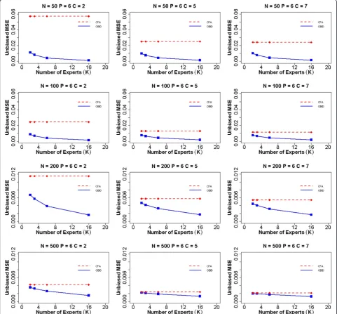
Figure 1 shows the average MSE of item-to-domain correlation ρ for unbiased experts when the number of items (P) is six. The participant sample sizes are

N =50, 100, 200, and 500. The numbers of response categories are C =2, 5, and 7, and the numbers of ex-perts are K =2, 3, 6, and 16. The MSE for CFA does not change with the number of experts (dashed line) as the expert content validity information is not uti-lized under the traditional approach. Thus the prior infor-mation has no effect on the CFA estimates across different choices for the number of experts. The OBID MSE (solid line) is consistently smaller than the CFA MSE, regardless of sample size and number of response categories, demonstrating the superior performance of the OBID approach. OBID is most promising for smaller sam-ples (e.g.,N =50 or 100). In addition, the OBID MSE de-creases as the number of experts inde-creases, with the largest reduction occurring approximately between 3–6 experts. When the number of response categories is bin-ary (C =2), we observe the largest vertical distance between the OBID MSE and the CFA MSE. This vertical distance reduces as the number of response categories in-crease, due to an increase in scale information. Similarly, the MSEs for both OBID and CFA decrease as the number of response categories increase; however, the MSE graphs for the five- and seven-point scales become very similar to each other across all sample sizes. It’s also expected that the MSEs for both approaches decrease as sample size in-creases, as a result of decreasing measurement errors. The asymptotic behavior of OBID is evaluated with sample size 500. As we expect, the two approaches produce almost identical MSEs with OBID being slightly smaller.

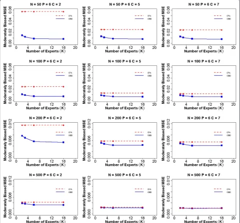
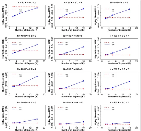
become smaller in the moderately biased case, indicating the effect of biased priors. Additionally, the efficiency gain of the OBID approach experiences a steady increase from 2–6 experts, and gradually levels off from 6–16 experts. This indicates that with moderately biased priors, having more than six experts does not contribute to any add-itional gain in the efficiency of OBID. When priors are highly biased (Fig. 3), our results support similar findings of BID [21] where the relative efficiency of OBID

compared with CFA is a function of the number of ex-perts. In the case of a binary response option and sample size 50, OBID produces smaller MSEs than CFA, despite of the receding efficiency as the number of experts in-creases. OBID is most efficient with smaller samples (e.g.,

similar patterns when the number of items is four or nine. MSE plots for additional simulation scenarios are included in Additional file 1: Figures S1–S6.

From simply observing the graphs, one may think that although OBID is more efficient, the performance of or-dinal CFA is comparable and not a bad choice. However, a close examination of the frequency that ordinal CFA failed to converge and/or produced “bad” estimates (i.e.,

ρj∉½1;1) reveals limitations of the classical method

samples. When the number of items is nine, the perform-ance of CFA becomes more stable with only 6 % out of bound estimates in the sample size 50 and binary response option case. The complete table that summarizes CFA performance can be found in Additional file 1: Table S1. In contrast, the OBID approach consistently produces ap-propriate and reliable correlation estimates without any challenges using all sample sizes and response options.

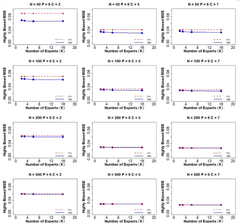
Lastly we assessed the predictive validity of the two ap-proaches under simulation settings. Under the previously

mentioned assumption, the criterion is perfectly measured (i.e., the ideal target); thus the correlation of test scores f_i

(i.e., the ability parameter) and criterion scores is the same as the validity coefficient corrected for attenuation in the criterion only. Figure 4 displays the MSEs of the validity co-efficientγcomputed using both OBID and CFA approaches when experts are highly biased and the number of items is six. Based on findings from Gajewski et al. [20], the subject experts tend to overestimate the relevancy of items, result-ing in highly biased item-to-domain correlations. The Fig. 3Average MSE of item-to-domain correlationρfor six items and highly biased experts. Average mean squared error (MSE) for item-to-do-main correlationρusing OBID (solid blue line) and ordinal CFA (dashed red line) whenP = 6(number of items) and experts are highly biased {ρ0¼ð0:65;0:75;0:85;0:85;0:65;0:75Þg. The participant sample sizes areN =50, 100, 200, and 500. The numbers of response categories are

predictive validity of OBID is examined in the extreme case of highly biased priors with a small sample size. For 50 par-ticipants, we can clearly observe that the MSE of OBID is the smallest with a binary response option (C = 2), com-pared with the CFA MSE. As number of response categor-ies increases, OBID continues to have smaller MSE than that of CFA, although the differences become much smaller and almost negligible. When we increase the sample size, the two approaches become almost identical in terms of MSEs. A similar trend is observed in the four item and nine item scenarios, with corresponding plots included in

Additional file 1: Figures S7–S14. Prior to the simulation, we hypothesize that MSEγ_OBID<MSEγ_CFA, fOBID is more correlated with fT than fCFA. The simulation results support this original hypothesis. Thus, we make the conclu-sion that OBID produces higher predictive validity than that of the traditional approach, especially for small samples.

Application to PAMS short form satisfaction survey data

medical center developed the patient assessment of mammography services (PAMS) satisfaction survey (four-factor with 20 items) and PAMS-Short Form (sin-gle factor with seven items) [32]. In this section, we apply the OBID approach to complete data collected from the PAMS-Short Form instrument that was ad-ministered to 2865 women: Hispanic (36, 1.26 %), Non-Hispanic white (2768, 96.61 %), African American (34, 1.19 %), and other (27, 0.94 %). Participants rated their satisfaction with each of the seven items using a five-point Likert-type scale, ranging from “poor” to “excel-lent.” In addition, six subject experts were consulted and instructed to evaluate each of the seven items on a four-point relevancy scale. The University of Kansas Medical Center’s Internal Review Board (IRB) has de-termined that our study does not require oversight by the Human Subjects Committee (HSC), as data were collected for prior studies and they are provided to us in a de-identified fashion.

Based on the sample size for each racial/ethnic group, establishing construct validity evidence for scores for Non-Hispanic white participants is clearly adequate and traditional CFA will suffice based on the large sample. Yet, researchers are interested in establishing score-based construct validity evidence for groups such as Hispanic/ African Americans which are typically small. Classical CFA is ill-suited for such small samples; thus we apply the OBID approach for the analyses of Hispanic/African American populations. For comparison purposes, we per-form OBID with experts’ opinions (informative) and OBID without experts’opinions (non-informative) due to estimation challenges with traditional CFA. Flat priors are assigned for the IRT model parameters in the OBID pos-terior non-informative cases, in which,αjeNð0;1Þandλje

Nð0;4Þ. In addition, based on trial and error we set the tuning parameter value required forMCMCpack to 2.00 for both small populations. The estimated item-to-domain correlationρ_jand its corresponding standard error are re-ported in Additional file 1: Table S2.

The non-informative OBID tends to overestimate ρ_j compared with the experts’estimated correlations (.381-.673), for both Hispanic (.570-.920) and African American (.774-.942) populations. By integrating the experts’ opin-ions with participants’ data, informative OBID produces more reliable results (Hispanic: .466-.717; African Ameri-can: .495-.725) by appropriately lowering the estimatedρ_j. Although not reported, the factor score or latent variable score for each participant (i.e., individual mammography satisfaction) also is estimated. Since the factor scores are adjusted or corrected for measurement error, patients can be more accurately classified into diagnostic groups based on factor scores, and then treated as covariates in subse-quent analyses. The non-informative OBID estimates tend

to have slightly smaller standard errors, which can be viewed as a trade-off between the overestimated reliability

ρ2

j and the variance. Overall, as we expect, OBID success-fully produces reliable item-to-domain correlation esti-mates and overcomes the small sample size challenge that often causes classical CFA to fail.

Discussion

As health care moves rapidly toward a patient-centeredness care model, the development of reliable and valid PROMs is recognized as an essential step in promoting quality care. Despite of increasing public awareness, the development of PROMs using trad-itional psychometric methodologies often is lengthy and constrained by the large sample size requirement, resulting in substantially increased costs and resources. In this study, an innovative OBID approach within a Bayes-ian IRT framework is proposed to overcome both small sample size (e.g., patients from small populations or rare diseases) and ordinal data modeling limitations. OBID seamlessly and efficiently utilizes subject experts’opinions (content validity) to form the prior distributions for the IRT parameters in construct validity analysis, as opposed to using arbitrarily selected priors in other Bayesian IRT simulation studies mentioned in the introduction.

samples, OBID proves to be an efficient and reliable approach.

One limitation of this study is associated with the source of experts’ information used in the PAMS-Short Form example. Opinions from the six content experts were originally consulted with the purpose of validating the PAMS instrument for the American Indian women population. Although the same set of survey items was administered to all American Indian, Hispanic, and African American populations, potential bias could be introduced due to the original focus of content experts. Nonetheless, as previously mentioned, reliable informa-tion collected from the six experts can still be utilized to form a“general prior”in establishing construct valid-ity for Hispanic and African American populations. An-other limitation of the study comes from the elicitation of content validity using relevance scales. Although Gajewski et al. [26] has demonstrated the appropriate-ness of measuring content validity using relevance scales, the equivalency with measuring content validity using correlation scales is approximate, which may have an effect on the parameter estimation. A third limita-tion of the study comes from the approximate normal distribution assumption that we made regarding the prior distribution of the experts after Fisher’s trans-formation. As pointed out by one of the reviewers, po-tential disagreements among selected subject experts may occur, which can cause the expert opinion to fol-low a bimodal (i.e., two groups of experts with opposite views) or even trimodal distribution. We acknowledge this limitation as this scenario was not examined in the current simulation study.

Two useful practical recommendations can be ex-tracted from the current study. As previously men-tioned, no standard method exist for determining appropriate tuning parameter values that ensure the 20-50 % acceptance rate needed for the MCMC pro-cedure. Although trial and error also is used in this study, our findings provide a general guideline for the selection of tuning parameter values. We find that tuning parameter values 1.00, 0.70, 0.50, and 0.30 appear to work well for sample sizes 50, 100, 200, and 500, respectively. Additionally, our study results are consistent with find-ings from Polit and Beck [33] regarding the number of subject experts needed to establish content validity. Across three types of expert biases, results show that having more than six experts does not contribute to any additional gain in the efficiency of OBID. With highly biased experts, three experts appear to be suffi-cient for establishing content validity.

An implication from this study is that a hierarchical model can be considered in the future to incorporate the individual effect of content experts, as the scores experts assigned from item to item are likely to be correlated. In

addition, the development of the user-friendly BID soft-ware can be used to guide the development of the OBID software, where multi-factor models can be evaluated, as it is common in many“long-form”questionnaires to en-compass several constructs of interest. It is our ultimate goal to extend the application capability of OBID and present it as an efficient and reliable method for re-searchers and clinicians in future PROMs development.

Conclusions

In this study, the efficiency of OBID is evaluated by comparing its performance to classical instrument devel-opment performance using actual and simulation data. This study successfully demonstrated that the OBID ap-proach is more efficient than the classical apap-proach when the sample size is small. OBID promises an effi-cient and reliable method for researchers and clinicians in future PROMs development for small populations or rare diseases.

Additional file

Additional file 1:Additional Simulation and Application Results. Additional simulation and application results referenced in Sections 3, 4 and 5. (PDF 901 kb)

Abbreviations

AERA:American Educational Research Association; APA: American Psychological Association; BID: Bayesian Instrument Development; CFA: confirmatory factor analysis; FDA: Food and Drug Administration; HSC: Human Subjects Committee; IOM: Institute of Medicine;

IACCV: Integrated Analysis of Content and Construct Validity; IRB: Internal Review Board; IRT: item response theory; MCMC: Markov chain Monte Carlo; MSE: Mean squared error; NCME: National Council on Measurement in Education; NIH: National Institute of Health; NQF: National Quality Forum; OBID: Ordinal Bayesian Instrument Development; PAMS: Patient assessment of mammography services; PCORI: Patient-Centered Outcomes Research Institute; PROMs: Patient-reported outcome measures; SEM: Structure equation modeling; DHHS: U. S. Department of Health and Human Services; WLSMV: Weighted least squares means- and variance-adjusted.

Competing interests

The authors declare that they have no competing interests.

Authors’contributions

LG conducted literature review, participated in the study design, simulated data, performed the statistical analysis, and drafted the manuscript. LP participated in the study design, provided feedback on simulation results and psychometric analyses, and provided critical manuscript revision. MB participated in the study design, provided feedback on simulation results, and provided critical manuscript revision. BG conceived of the study, conducted literature review, initiated the study design and implementation, reviewed all statistical analyses and simulation results, and provided critical manuscript revision. All authors contributed to and approved the final manuscript.

Authors' information Not applicable.

Acknowledgments

Funding

Research reported in this publication was supported by the National Institute of Nursing Research of the National Institutes of Health under Award Number R03NR013236. The content is solely the responsibility of the authors and does not necessarily represent the official views of the National Institutes of Health. Data from PAMS come from P20MD004805.

Author details

1_{Department of Biostatistics, University of Kansas Medical Center, Mail Stop}

1026, 3901 Rainbow Blvd., Kansas City, KS 66160, USA.2College of Education, Texas State University, San Marcos, TX 78666, USA.3_{University of Kansas}

School of Nursing, Mail Stop 4043, 3901 Rainbow Blvd., Kansas City, KS 66160, USA.

Received: 5 May 2015 Accepted: 21 September 2015

References

1. Institute of Medicine. Crossing the Quality Chasm: A New Health System for the 21st Century. Washington, DC: National Academy Press; 2001. 2. Cella D, Riley W, Stone A, Rothrock N, Reeve B, Yount S, et al. The

Patient-Reported Outcomes Measurement Information System (PROMIS) developed and tested its first wave of adult self-reported health outcome item banks: 2005–2008. J Clin Epidemiol. 2010;63(11):1179–94.

3. US Department of Health and Human Services Food and Drug

Administration. Guidance for Industry Patient-Reported Outcome Measures: Use in Medical Product Development to Support Labeling Claims. 2009. 4. National Quality Forum. Patient Reported Outcomes (PROs) in Performance

Measurement. 2013.

5. Patient Centered Outcomes Research Institute. The Design and Selection of Patient-Reported Outcomes Measures (PROMs) for Use in Patient Centered Outcomes Research. 2012.

6. Pett MA, Lackey NR, Sullivan JJ. Making sense of factor analysis: The use of factor analysis for instrument development in health care research. Thousand Oaks: Sage; 2003.

7. Johnson VE, Albert JH. Ordinal data modeling. New York: Springer Science & Business Media; 1999.

8. American Educational Research Association, American Psychological Association, National Council on Measurement in Education. Standards for Educational and Psychological Testing. Washington, DC: AERA; 2014. 9. Nunnally IH, Bernstein JC. Psychometric theory. New York: McGraw-Hill; 1994. 10. Messick S. Validity. In: Linn RL, editor. Educational Measurement. 3rd ed.

New York: American Council on Education; 1989. p. 13–103.

11. Knapp TR, Brown JK. Ten measurement commandments that often should be broken. Res Nurs Health. 1995;18:465–9.

12. Thurstone LL. Multiple factor analysis. Chicago: Chicago University of Chicago Press; 1947.

13. Brown TA. Confirmatory factor analysis for applied research. 2nd ed. New York: Guilford Publications; 2014.

14. Anthoine E, Moret L, Regnault A, Sébille V, Hardouin JB. Sample size used to validate a scale: a review of publications on newly-developed patient reported outcomes measures. Health Qual Life Outcomes. 2014;12:176. 15. Weenink JW, Braspenning J, Wensing M. Patient reported outcome

measures (PROMs) in primary care: an observational pilot study of seven generic instruments. BMC Fam Pract. 2014;15:88.

16. Knapp TR. Treating ordinal scales as interval scales: an attempt to resolve the controversy. Nurs Res. 1990;39:121–3.

17. Muthén B. A general structural equation model with dichotomous, ordered categorical, and continuous latent variable indicators. Psychometrika. 1984;49:115–32.

18. Rosseel Y. lavaan: an R package for structural equation modeling. J Stat Softw. 2012;48:1_–36.

19. R Core Team. R: A language and environment for statistical computing. In. Vienna, Austria: R Foundation for Statistical Computing; 2014.

20. Gajewski BJ, Price LR, Coffland V, Boyle DK, Bott MJ. Integrated analysis of content and construct validity of psychometric instruments. Qual Quant. 2013;47:57–78.

21. Jiang Y, Boyle DK, Bott MJ, Wick JA, Yu Q, Gajewski BJ. Expediting clinical and translational research via Bayesian instrument development. Appl Psychol Meas. 2014;38:296–310.

22. Arima S. Item selection via Bayesian IRT models. Stat Med. 2015;34(3):487–503. 23. Fox JP, Glas CAW. Bayesian estimation of a multilevel IRT model using Gibbs

sampling. Psychometrika. 2001;66(2):271–88.

24. Price LR. Psychometric Methods: Theory into Practice. New York, NY: Guilford Publications; in press.

25. Quinn KM. Bayesian factor analysis for mixed ordinal and continuous responses. Polit Anal. 2004;12(4):338–53.

26. Gajewski BJ, Coffland V, Boyle DK, Bott M, Price LR, Leopold J, et al. Assessing content validity through correlation and relevance tools a Bayesian randomized equivalence experiment. Methodology-Eur. 2012;8(3):81–96.

27. Cohen J. Statistical power analysis for the behavioral sciences. Hillsdale, NJ: Erlbaum; 1988.

28. Lunn DJ, Thomas A, Best N, Spiegelhalter D. WinBUGS - a Bayesian modelling framework: concepts, structure, and extensibility. Stat Comput. 2000;10(4):325–37.

29. Martin AD, Quinn KM, Park JH. MCMCpack: Markov Chain Monte Carlo in R. J Stat Softw. 2011;42(9):1–21.

30. Cowles MK. Accelerating Monte Carlo Markov chain convergence for cumulative-link generalized linear models. Stat Comput. 1996;6(2):101–11. 31. Gelman A, Carlin JB, Stern HS, Rubin DB. Bayesian data analysis. Texts in

statistical science series. 2004.

32. Engelman KK, Daley CM, Gajewski BJ, Ndikum-Moffor F, Faseru B, Braiuca S, et al. An assessment of American Indian women's mammography experiences. BMC women's health. 2010;10(1):34.

33. Polit DF, Beck CT. The content validity index: are you sure you know what’s being reported? Critique and recommendations. Res Nurs Health. 2006;29:489–97.

Submit your next manuscript to BioMed Central and take full advantage of:

• Convenient online submission

• Thorough peer review

• No space constraints or color figure charges

• Immediate publication on acceptance

• Inclusion in PubMed, CAS, Scopus and Google Scholar

• Research which is freely available for redistribution