Quasiperiodic ULF-pulsations in Saturn’s magnetosphere

www.ann-geophys.net/27/885/2009/

© Author(s) 2009. This work is distributed under the Creative Commons Attribution 3.0 License.

Annales

Geophysicae

Quasiperiodic ULF-pulsations in Saturn’s magnetosphere

G. Kleindienst1, K.-H. Glassmeier1,2, S. Simon3,*, M. K. Dougherty4, and N. Krupp2

1_{Institut f¨ur Geophysik und extraterrestrische Physik, Technische Universit¨at Braunschweig, Mendelssohnstraße 3,}

38106 Braunschweig, Germany

2_{Max-Planck-Institut f¨ur Sonnensystemforschung, Max-Planck-Straße 2, 37191 Katlenburg-Lindau, Germany}

3_{Institut f¨ur Theoretische Physik, Technische Univ. Braunschweig, Mendelssohnstraße 3, 38106 Braunschweig, Germany} 4_{The Blackett Laboratory, Imperial College London, Prince Consort Road, London SW7 2BW, UK}

*_{now at: Universit¨at zu K¨oln, Institut f¨ur Geophysik und Meteorologie, Z¨ulpicher Str. 49a, 50674 K¨oln, Germany}

Received: 16 June 2008 – Revised: 18 December 2008 – Accepted: 27 January 2009 – Published: 23 February 2009

Abstract. Recent magnetic field investigations made on-board the Cassini spacecraft in the magnetosphere of Saturn show the existence of a variety of ultra low frequency plasma waves. Their frequencies suggest that they are presumably not eigenoscillations of the entire magnetospheric system, but excitations confined to selected regions of the magne-tosphere. While the main magnetic field of Saturn shows a distinct large scale modulation of approximately 2 nT with a periodicity close to Saturn’s rotation period, these ULF pul-sations are less obvious superimposed oscillations with an amplitude generally not larger than 3 nT and show a package-like structure. We have analyzed these wave packages and found that they are correlated to a certain extent with the large scale modulation of the main magnetic field. The spa-tial localization of the ULF wave activity is represented with respect to local time and Kronographic coordinates. For this purpose we introduce a method to correct the Kronographic longitude with respect to a rotation period different from its IAU definition. The observed wave packages occur in all magnetospheric regions independent of local time, elevation, or radial distance. Independent of the longitude correction applied the wave packages do not occur in an accentuated Kronographic longitude range, which implies that the waves are not excited or confined in the same selected longitude ranges at all times or that their lifetime leads to a variable phase with respect to the longitudes where they have been exited.

Keywords. Magnetospheric physics (Magnetospheric con-figuration and dynamics; MHD waves and instabilities; Plan-etary magnetospheres)

Correspondence to: G. Kleindienst ([email protected])

1 Introduction

ULF waves are a widely observed phenomenon in various en-vironments of the solar system. At comets pick-up of newly-ionized particles leads to the generation of low-frequency waves at the local ion-gyro frequency (e.g. Tsurutani and Smith, 1986; Glassmeier and Neubauer, 1993; Glassmeier et al., 1993). The solar wind interaction regions of plan-ets Venus and Mars are also prone to the generation of low-frequency waves by pick-up ions (e.g. Luhmann et al., 1983; Espley et al., 2004). The terrestrial magnetosphere, how-ever, is the classical environment to study ULF waves and eigenoscillations of an entire magnetosphere (e.g. South-wood and Hughes, 1983). Typical source mechanisms are the Kelvin-Helmholtz instability (e.g. Fujita et al., 1996), ring-current instabilities (e.g. Southwood, 1976), or solar wind buffeting (e.g. Mathie and Mann, 2000).

Apart from the well studied ULF waves in the Earth’s magnetosphere, ULF waves can also be found in the mag-netospheres of Mercury and the gaseous planets Jupiter and Saturn (e.g. Glassmeier et al., 2004). Khurana and Kivel-son (1989) analyzed ULF waves confined in the equatorial region of the Jovian magnetosphere, while Glassmeier et al. (1989) reported about MHD waves confined to the Io plasma torus. Based on magnetic field investigations from Voy-ager 2, Cramm et al. (1998) showed evidence of ULF waves and resonant mode coupling in Saturn’s magnetosphere.

r

B [nT]

|B| [nT]

Day of Year

MFA

2004, December 18

2004, December 15−21

Cassini (FGM)

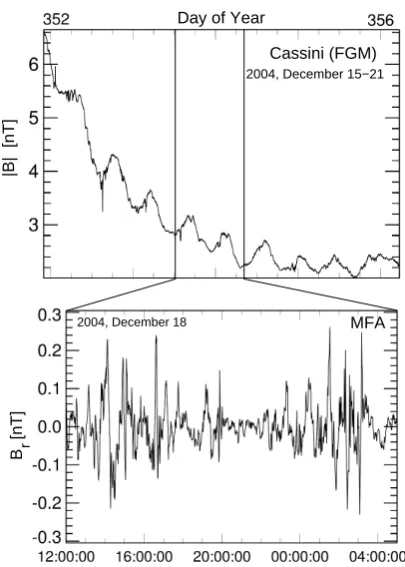
Fig. 1. Upper panel: magnitude of the main magnetic field over time (15–21 December 2004); bottom panel: the radial component of the magnetic field in a mean-field-aligned coordinate system, dis-playing two of the typical ULF waves packages centered around 18 December 2004, 15:00 UTC and 19 December 2004, 02:00 UTC.

the generation of standing toroidal magnetic field oscilla-tions, the application of the field-line resonance theory to the Jovian and Kronian magnetosphere needs further analysis.

Recent studies based on the magnetic field investigation (Dougherty et al., 2004) of the Cassini mission into the Kro-nian system exhibit a variety of periodic magnetospheric per-turbations at Saturn, amongst others a modulation of the magnetic field with a period close to the planetary rotation period (Giampieri et al., 2006), which has already been ob-served by the magnetometer experiments onboard the Voy-ager 1, VoyVoy-ager 2 and Pioneer 11 spacecraft as a reanaly-sis of their magnetic field data demonstrates (Espinosa and Dougherty, 2000; Espinosa et al., 2003a). Giampieri et al. (2006) used this periodicity to derive a rotation period based on magnetic field measurements and yielded a period of 10 h 47 min 6 s which differs significantly from the rotation period of 10 h 39 min 22 s as officially defined by the IAU (Seidelmann et al., 2002) relying on earlier measurements by Desch and Kaiser (1981), based on the periodic occurrence of kilometric radiation in Saturn’s high latitude regions.

The reported existence of magnetohydrodynamic waves in the magnetospheres of the gaseous planets as well as the ini-tial findings of Espinosa et al. (2003b) and Giampieri et al.

(2006) motivated the present work. In the terrestrial mag-netosphere several source mechanisms for ULF waves are known, while at Jupiter and Saturn knowledge about the wave source is still sparse.

Glassmeier (1995) suggested that the tilted and rotat-ing Jovian dipole axis causes large-amplitude and periodic magnetic field perturbations in the Jovian magnetosphere whose non-linear decay is able to generate a variety of low-frequency wave phenomena. As the magnetic dipole axis of Saturn is almost aligned with the rotation axis of the planet a direct extension of the suggestion of Glassmeier (1995) to the Kronian system is not possible. However, the large scale modulation of the Kronian magnetic field, whatever cause it has, can be regarded as a similar large-amplitude wave per-turbation, which can be the source of ULF waves at Saturn. In the present study we thus concentrate on general wave properties and the spatial localization of the ULF waves in the Kronian magnetosphere and their relation to so far dis-covered magnetic features such as the periodic modulation of Saturn’s main magnetic field. The frequency of the ob-served ULF pulsations indicates that they are not eigenoscil-lations of the entire Kronian magnetosphere, but are due to waves bound to specific regions of the magnetosphere. The identification of these regions is hampered by the definition of the Kronian longitude system (Seidelmann et al., 2002), which depends strongly on the accuracy of the planet’s rota-tion period, which is just under discussion (Giampieri et al., 2006; Cecconi and Zarka, 2005; Gurnett et al., 2007; Gol-dreich and Farmer, 2007; Southwood and Kivelson, 2007). Thus, one of the aims of our study is also to find a suitable coordinate system, in which the observed ULF waves can best be represented, to understand their basic characteristics and to relate their occurrence to the global structure of the Kronian magnetosphere.

2 ULF wave properties

We analyse measurements from the vector fluxgate magne-tometer of the Cassini spacecraft (Dougherty et al., 2004). For the present study we use magnetic field data with an av-eraged time resolution of 1 min along the path of the space-craft’s outbound trajectory from July 2004 to March 2007, inside the magnetosphere of Saturn, which corresponds to the first 40 revolutions of the spacecraft around the planet.

The spacecraft covered all local time ranges during this pe-riod of time and its orbits were close to the magnetic equator within a latitude range of±20◦ _{for nearly 80% of the total}

time under consideration. Radial ranges from 3RSto 50RS

were covered by the path of the satellite.

frequencies in the range of 5−10 mHz for a background mag-netic field of 10 nT. Thus, the observation of magnetohydro-dynamic waves should be covered well enough by the chosen time resolution.

Figure 1 displays a typical example of the ULF waves ana-lyzed. The oscillations are rather irregular and do usually not exhibit any quasi-sinusoidal character as often observed in the terrestrial magnetosphere. The wave activity is strongly modulated and resembles a certain correlation with varia-tions of the background magnetic field. To access and distin-guish these small amplitude oscillations from the background magnetic field and to distinguish oscillations transverse and parallel to the background magnetic field, we transform the magnetic field data into a Mean-Field-Aligned (MFA) co-ordinate system (er,eφ,ek), whereekdenotes the unit

vec-tor in the direction of the background magnetic field,eφthe

unit vector perpendicular to the plane spanned byekand the spacecraft position vectorrsc. The unit vectorer completes

the right hand (er,eφ,ek) triad. The coordinate system used

is thus defined as follows:

er =eφ×ek (1)

eφ=

hBi ×rsc

|hBi ×rsc|

(2)

ek= hBi

|B|. (3)

The mean magnetic fieldhBiis determined by a second order polynominal fit within a sliding window of 141 min width, whose window size comprises the large scale modulation of the background magnetic field well. In the MFA-system (br, bφ, bk) denotes the magnetic disturbance field vectors.

As we are only interested in field perturbations the mean value of the field-aligned component has been subtracted. The MFA-system allows one to inspect also the polarization of the analysed oscillations with (br, bφ, bk) approximately

describing poloidal, toroidal, and field-aligned components, respectively.

A series of clearly distinguishable wave packages with mainly transverse amplitudes generally not larger than 0.5 nT can be observed in the components perpendicular to the mean magnetic field for the chosen time interval. Figure 1 shows an interval of increased ULF wave activity as an example which exhibits two of the package-like structures centered around 18 December 2004, 15:00 UTC and 19 December 2004, 02:00 UTC, respectively.

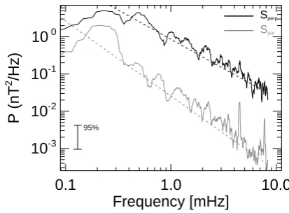
The predominance of transverse over compressional fluc-tuations can be inferred from a spectral analysis of the two different components. Figure 2 shows a sample spectrum for the time interval 18 December 2004, 12:00 until 19 De-cember 2004, 05:04 UT. The power spectral density distri-bution is rather featureless, does not exhibit any clear spec-tral peak being larger than the confidence limit, and decays with a spectral index of about−5/3. The perpendicular spec-tral density is at least an order of magnitude larger than the

0.1

1.0

10.0

Frequency [mHz]

10

10

10

10

P (nT

2

/Hz)

95%

Sperp

Spar

Fig. 2. Power spectral density of the ULF wave activity in the time interval 18 December 2004, 12:00 UTC to 19 December 2004, 05:04 UTC. The black line represents the sum of the spectral power density of the magnetic field fluctuations perpendicular to the back-ground magnetic field. The grey line shows the spectral power den-sity of the magnetic field fluctuations parallel to the background magnetic field. The dashed lines illustrate the spectral slopes fitted to each spectral power density.

parallel one. Therefore we classify the observed ULF wave activities as Alfv´enic fluctuations.

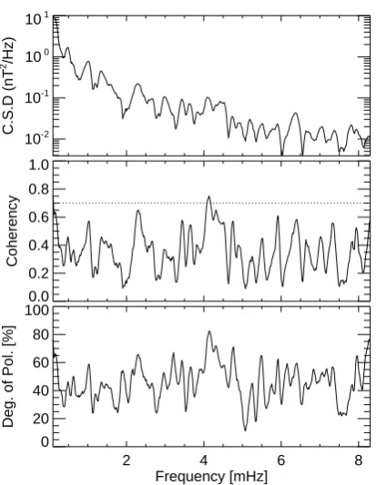
The cross-spectral density which was calculated for the two transverse componentsBr andBφof the magnetic field

represented in Fig. 3 shows, that no maximum is clearly ac-centuated from the background spectrum and the coherency has values generally much smaller then γ=0.7, which im-plies that the degree of polarization in the plane perpendic-ular to the background magnetic field is also small. Before investigating this correlation any further we like to comment on any wave activity distribution as observed in the Kronian magnetosphere.

Because of the rather irregular level of fluctuations we use the Carson-Gabor or analytical signal representation (Glass-meier, 1980) to yield an instantaneous amplitude of the mag-netic field oscillations in order to determine and calculate a wave activity index. In this representationz(t )=x(t )+iy(t ) is a complex time series withx(t )representing the original time series andy(t )being defined as

y(t )=H(x(t )), (4)

whereHdenotes the Hilbert-transform. The instantaneous amplitudeA(t )is now given as

A(t )=

q

x2_{(t )+y}2_{(t ). (5)}

We define a wave activity indexW (t )for each magnetic field component as the hourly time average of the instantaneous amplitude. As an example Fig. 4 displays the radial variation of the transverse wave index, W⊥=(Wr+Wφ)/2, together

10-2

10-1

10 0

10 1

C.S.D (nT

2 /Hz)

0.0 0.2 0.4 0.6 0.8 1.0

Coherency

2 4 6 8

Frequency [mHz] 0

20 40 60 80 100

Deg. of Pol. [%]

Fig. 3. The cross spectral density of the ULF wave packages in the time interval from 18 December 2004, 12:00 UTC and 19 December 2004, 05:04 UTC for the two transverse magnetic field components.

function of radial distance for the time interval 15 December 2004–22 December 2004; indices denote the magnetic field components used. Apparently the wave activity correlates with the large scale variation of the magnetic field strength. To quantify this possible correlation we formally determine the cross correlation function between both time series. To remove the trend of the total magnetic field we have fitted a dipolar declining function to the minima of the total field ra-dial variation. The resulting residuum is correlated with the wave activity index for a maximum lag of 1500 min. The first local maximum occurs for a lag time of approximately−2 h, that is the background magnetic field reaches its maximum two hours after the wave activity maximizes. The cross-correlation function shows a clear periodic structure with a maximum correlation coefficient of about 0.5. This correla-tion coefficient is lower than anticipated by visual inspeccorrela-tion of Fig. 4 and due to variations of the instantaneous amplitude at around 24RS and 37RS. Correlating the two time series

between 26RS and 35RS gives one a maximum correlation

coefficient of 0.75 and a corresponding lag time of−98 min (Fig. 5). We conclude that there is an interesting relation be-tween ULF wave activity and the variation of the background magnetic field.

To further analyze the wave activity distribution we use the data in the MFA-system to calculate the total wave activity indexWtot=1₃(Wr+Wφ+Wk), the transverse wave activity

2.00 2.50 3.00 3.50 4.00 4.50 5.00

|B| [nT]

25 30 35 40

Radial Distance [RS]

0.00 0.02 0.04 0.06 0.08 0.10 0.12

Instantaneous Amplitude [nT]

Fig. 4. Upper panel: magnitude of the main magnetic field over radial distance in the time interval from 17 December 2004, 06:00 UTC and 21 December 2004, 03:00 UTC. The dashed line shows the trend which has be subtracted from the magnetic field magnitude for further correlation analysis. Bottom panel: trans-verse wave activity indexW⊥over radial distance.

indexW⊥, and the parallel wave activity indexWkfor those

time intervals, where the spacecraft was inside Saturn’s mag-netosphere. Wave activity distribution functions are deter-mined using a bin size of 0.1 nT. The resulting distributions in Fig. 6 indicate, that for all three indices the wave activ-ity index declines exponentially for larger indices. The to-tal wave index distribution shows that most fluctuations have small amplitudes, generally not larger than 3 nT, which are all situated well above the instrumental noise-level which is stated to be better than 25 pT2/Hz (Dougherty et al., 2004).

The transverse and compressible distributions bear a sim-ilar feature. For wave indices less than 0.5 nT we observe a higher number of transverse wave indices as compared to parallel wave indices, while for larger amplitudes up to 1.5 nT both polarizations contribute equally. For amplitudes larger than 1.5 nT the number of parallel wave indices are slightly larger compared to the transverse wave indices.

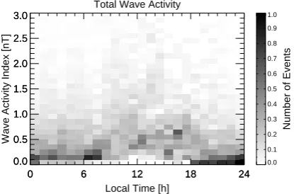
To investigate a possible dependence of wave activity on the magnetospheric regions they have been detected in, we calculated distributions of the total wave activity index with respect to magnetic local time, radial distance, and magnetic elevation.

-1000 -500 0 500 1000 Time-lag [min]

-1.0 -0.5 0.0 0.5 1.0

Cross-Correlation P

xy

Fig. 5. Cross-Correlation of the detrended magnitude of the mag-netic field and the wave activity index for the subinterval of the time series depicted in Fig. 4 restricted to the the radial range between 26RSand 35RS. The first maximum peaks at a time-lag of approx.

100 min. A negative time-lag implies that the detrended magnitude of the magnetic field has to be shifted backwards in time to show a maximum correlation with the instantaneous amplitude of the wave activity index, thus appearing along the rising flanks of the magnetic magnitude.

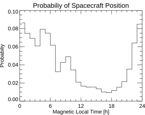
local time region with respect to a binsize of 1 h. Such a normalized distribution (Fig. 8) exhibits that wave activity indices are generally not larger than 1 nT and more or less uniformly distributed over magnetic local times. There is a slight indication for larger amplitudes of about 0.5 nT around local noon. However we do not regard this as a significant structure and would like to conclude a rather equal local time distribution from the observed distribution. In a similar way we also determine normalized distributions as a function of radial distance and magnetic elevation. The radial distribu-tion is almost uniform over all radial distances with wave ac-tivity indices generally not larger than 0.5 nT. The magnetic elevation dependent normalized distribution indicates only a minor enhancement for magnetic elevations larger than±30◦ and is uniform otherwise. The minor enhancement is most probably an artifact, as the spacecraft’s probability distribu-tion is fairly low for these elevadistribu-tions and thus the normal-ized distribution is over-emphasnormal-ized for elevations beyond ±30◦_{. We thus conclude that ULF wave activity of}

com-parable magnitude is observed all over the magnetospheric regions visited by Cassini so far.

3 ULF wave activity and a rotation-related coordinate system

The relation between background magnetic field and ULF wave activity suggested by the results presented in Figs. 4 and 5 deserves further attention as we found similar correlations also for other time intervals.

To further our hypotheses it is desirable to represent the wave activity in a rotation-related coordinate system. The spacecraft’s position with respect to standard Kronographic

0.5 1.0 1.5 2.0 2.5 3.0

Wave Activity Index [nT] 1

10 100 1000

Number of Events

Fig. 6. Wave activity index distributions: the dashed lines gives the distribution of the total wave activity index, the solid one that of the tranverse oscillations, and the dotted line denotes the compressible perturbation index. The one hour time average of the wave activity index is counted as one event in the statistic.

Probabiliy of Spacecraft Position

0 6 12 18 24

Magnetic Local Time [h] 0.00

0.02 0.04 0.06 0.08 0.10

Probabiliy

Fig. 7. Histogram of the probability to find the spacecraft within a magnetic local time range, which is used to normalize the distribu-tion of the hourly averaged total wave activity index with respect to their amplitude and magnetic local time.

0 6 12 18 24 0.0

0.5 1.0 1.5 2.0 2.5 3.0

0 6 12 18 24

0.0 0.5 1.0 1.5 2.0 2.5 3.0

0.0 0.1 0.2 0.3 0.4 0.5 0.6 0.7 0.8 0.9 1.0

Number of Events

Local Time [h]

Wave Activity Index [nT]

Total Wave Activity

Fig. 8. The histogram shows the number of wave events of the hourly averaged total wave activity index with respect to their am-plitude and magnetic local time distribution. The local time distri-bution has been normalized with the probability distridistri-bution of the spacecraft’s local time position. The resulting histogram is normal-ized to one. The histogram does not show any region of pronounced wave activity and the number of wave indices is more uniformly dis-tributed then before the normalization. Only a slight indication for an enhanced wave activity with marginal larger amplitudes may be observed around local noon.

given by the IAU (Seidelmann et al., 2002). This differ-ence between the IAU and Giampieri et al. (2006) rotation periods indicates a variable apparent Kronian rotation rate. As a consequence Giampieri et al. (2006) suggested to cor-rect the Saturn prime meridian and the rotation period ac-cordingly. Any localization of physical processes such as the observed wave activity with respect to Kronian longi-tude will become obsolete if an incorrect rotation rate and longitude system is used. Therefore we need to correct the longitude of any wave activity observation with respect to the new, magnetic field based rotation period. The simplest method to introduce the required correction is to consider the phase shift of the prime meridian arising from the difference betweenTIAU=10 h 39 min 22 s andTCassini=10 h 47 min 6 s.

If the longitude of the prime meridian at the beginning of the J2000 epoch (1 January 2000, 12:00:00 UT) isϕ0=38.90◦

(Seidelmann et al., 2002), the phase evolution due to the two differing rotation periods, TCassini and TIAU, can be

calcu-lated. In the following the rotation rateω=360◦/T (◦/s)is used for further considerations. We first consider the phase evolution of the prime meridian due to a constant defined ro-tation rateωIAUand due to a variable rotation rateωKrono(t ):

ϕIAU(t )=ϕ0(t0)+ωIAU(t−t0) (6)

ϕKrono(t )=ϕ0(t0)+

Z t

t0

ωKrono(τ )dτ (7)

wheret is the time elapsed since t0. Obviously the prime

meridian has a different time evolution for the two rotation rates and the phase difference between them can be expressed

as

ϕKrono(t )=ϕIAU(t )+1ϕ(t ) (8)

1ϕ(t )=ϕKrono(t )−ϕIAU(t ) (9)

=

Z t

t0

ωKrono(τ )dτ −ωIAU(t−t0) . (10)

Any Kronographic longitudeλIAUcalculated on the basis of ωIAUneeds to be corrected with respect to this phase

differ-ence 1ϕ(t )in order to obtain a modified longitudeλKrono

which is stationary with respect to the prime meridian at ϕKrono(t ). The corrected longitude in the modified

Krono-graphic coordinate system thus reads:

λKrono(t )=λIAU(t )+1ϕ(t ) (11)

λKrono(t )=λIAU(t )−ωIAU(t−t0)+

Z t

t0

ωKrono(τ )dτ (12)

If one assumes that ωKrono is constant in time and

the prime meridians were congruent at t0, the phase

shift between a prime meridian calculated with respect

to ωIAU=9.384×10−3◦/s (TIAU=10 h 39 min 22 s) and

ωCassini=9.272×10−3◦/s (TCassini=10 h 47 min 6 s)is

1ϕ(t )=ϕKrono(t )−ϕIAU(t ) (13)

=ωKrono(t−t0)−ωIAU(t−t0) (14)

=(ωKrono−ωIAU)

| {z }

1ω

(t−t0) . (15)

with1ω=−0.1127×10−3◦/s(1T=7 min 44 s). This leads to a phase shift of the prime meridian of 4.3◦ per nominal rotation and sums up to a complete rotation every 37.2 days. The longitude determined with any standard tool such as the NAIF Toolkit is easily corrected by adding the phase shift of the prime meridian:

λKrono(t )=λIAU(t )+1ϕ(t ) (16)

Longitudes corrected in this way are used to infer any local-ization of the observed ULF waves in a Kronographic coor-dinate system.

Appearance of Maximum Wave Activity

0 10 20 30 40 50

Radial Distance [RS]

0 90 180 270 360

Kronographic Longitude [deg]

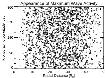
Fig. 9. Position of the maxima of the wave activity index in krono-graphic longitude over radial distance based on the rotation period of 10 h 39 min 22 s defined by the IAU (Seidelmann et al., 2002).

λS,Krono(t )=λS,IAU(t )+1ϕ(t ) (17)

=λS,IAU(t )+

Z t

t0

ωKrono(τ )dτ−ωIAU(t−t0)

.

(18) From this the time derivative ofλS,IAU(t )as well as the true

rotation period can be determined, because dλS,Krono/dt=0

for a stationary source: dλS,IAU(t )

dt = − ωKrono(t )−ωIAU

(19) ωKrono(t )=ωIAU−

dλS,IAU(t )

dt . (20)

The above considerations are used to study any possible lo-calization of the wave activity in the Kronian magnetosphere and its relation to the modulation of the background mag-netic field. For the time interval July 2004–January 2007 the maxima of the activity index are shown as a function of the standard Kronographic longitudeλand radial distanceR from the planet (Fig. 9). A total number of 1630 maxima of the total wave activity index have been selected by an auto-matic algorithm.

No structured distribution is observed, but the wave ac-tivity maxima are uniformly scattered in longitude and radial distance. Correcting the longitude as discussed above and us-ing the rotation period suggested by Giampieri et al. (2006) yields a slightly different distribution (not shown here), but still an almost uniform one. This either implies that the source of the wave activity is not stationary, or it hints to-wards a variable rotation rate. To check this later possibil-ity we derive a variable rotation rate based on the modula-tion of the z-component of the background magnetic field, which best exhibits the periodic variations of the magnetic

0 200 400 600 800 1000

Time since 2004-07-01T00:00:00 [d] 0

90 180 270 360

Longitude [deg]

Fig. 10. Longitude representation of the maxima of the z-component of the magnetic field modulation based on a rotation period of 10 h 47 min 6 s according to the results of Giampieri et al. (2006). The grey lines mark the regions to be shifted by an integer multiple of 360◦to produce the continous longitude representation of the displayed maxima. The time axis starts on day 2004-148.

0 200 400 600 800 1000

Time since 2004-07-01T00:00:00 [d] 0

360 720 1080 1440 1800

Longitude [deg]

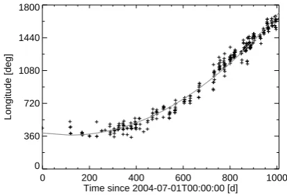
Fig. 11. Longitude representation of the maxima of the z-component of the magnetic field modulation based on a rotation period of 10 h 47 min 6 s according to the results of Giampieri et al. (2006) with data points shifted byn·360◦, n∈{0,1,2, . . .}in the selected regions divided by the grey lines in Fig. 10 to obtain a con-tinuous representation of the maxima without phase jumps at 360◦. The line represents the best fit model for a polynominal function to describe the drift-curve due to an erroneous rotation period. The time axis starts on day 2004-148.

0 200 400 600 800 1000 Time since 2004-07-01T00:00:00 [d]

-360 -270 -180 -90 0 90 180 270 360

Residual Longitude [deg]

Fig. 12. Longitude representation of the maxima of the z-component of the magnetic field modulation after removal of the fitted driftcurve to the datapoints, thus correcting the observed lon-gitudes with respect to a time-varying rotation period. The time axis starts on day 2004-148.

drifting in longitude or a still incorrect rotation rate is used. If this latter hypothesis is correct a time-varying rotation period needs to be assumed. To determine the apparent temporal variation of the rotation frequency we have fitted a quadratic function of the form

λBz,max(t )=λ0+α·t+β·(t−t0)

2 ₍₂₁₎

to the curve displayed in Fig. 11. The following parameters are found:

λ0=(34.09±15.3)◦ (22)

α=(1.37±1.70)×10−5◦/s (23)

β =(2.283±0.077)×10−13◦/s2 (24)

t0=(40622810±373500)s≈(470 ± 4.3)d (25)

where the timetis counted in s since 1 July 2004, 00:00 UT. With

ωKrono(t )=ωCassini−

dλBz,max(t )

dt (26)

=ωCassini− α+2β(t−t0)

(27) we obtain a rotation rate

9.278×10−5◦/s> ωKrono(t ) >9.238×10−5◦/s

(38 800 s< TKrono<38 970 s) for the beginning (1 July

2004) and the end (30 January 2007) of the considered time interval for the longitude drift.

With this variable rotation rate we can also correct the longitude-time distribution of the background magnetic mod-ulation (Fig. 12). Though considerable scattering is still ap-parent, the putative source location of the disturber caus-ing the background magnetic field modulation is well con-strained. The time-varying rotation rate and period function can also be extrapolated to past times to enable a comparison with earlier measurements of the rotation rate by e.g. Voy-ager 1. For the year 1980 a rotation period ofT=37 366 s

Appearance of Maximum Wave Activity

0 10 20 30 40 50

Radial Distance [RS]

0 90 180 270 360

Kronographic Longitude [deg]

Fig. 13. Position of the maxima of the wave activity index in krono-graphic longitude over radial distance based on a variable rotation period.

is determined in this way. This value clearly deviates from the earlier determined and IAU-accepted value. Thus, the suggested model for a time-varying rotation rate is only ap-plicable to the time interval covered by the Cassini mission so far.

Using the above derived apparent time-varying rotation rate the wave activity maxima and their relation to corrected Kronian longitude can be further discussed. Figure 13 dis-plays the resulting distribution. It is as featureless as the un-corrected distribution.

4 Summary and conclusion

the modulation excited the observed waves in an individual region of the Kronian magnetosphere.

Furthermore we seized the suggestion made by Giampieri et al. (2006) to correct the Kronian longitude system with respect to a new rotation rate and introduced a simple correction method based on the phase evolution of Saturn’s prime meridian for two different rotation periods. The appli-cation of this method did not organize the longitude distribu-tion of the ULF wave activity within distinguishable regions of preference, but it revealed a clear longitudinal drift of the maxima of the magnetic field modulation (Fig. 10) which suggests a time-variable period of the perturbation.

Therefore a time-variable kronographic longitude system was derived, based on the z-component of the magnetic field data, assuming a variable rotation period. The rotating sys-tem found well orders the background magnetic field modu-lation within an accentuated longitude range, hence indicat-ing a suitable kronographic longitude system for the repre-sentation of the ULF wave activity. However, the application of this longitude system to represent the ULF wave activity information does not yield any systematic longitude distribu-tion (Fig. 13). This quesdistribu-tions our hypothesis.

Nevertheless, the simple model of an eccentric excitation and subsequent decay of a large amplitude perturbation needs more detailed considerations. A detailed model is required to take propagation effects within the magnetosphere, local conditions for the excitation of ULF waves in selected re-gions and considerations concerning the life-time of ULF waves in those special regions into account. Such consid-erations are beyond the scope of the present study.

Finally, we like to note that our time-variable Kronian lon-gitude system is comparable to that one recently introduced by Kurth et al. (2007).

Acknowledgements. This work was financially supported by the German Bundesministerium f¨ur Wirtschaft und Technologie and the Deutsches Zentrum f¨ur Luft- und Raumfahrt under con-tract 50 OH 9901/4.

Topical Editor I. A. Daglis thanks two anonymous referees for their help in evaluating this paper.

References

Acton, C. H.: SPICE Products Available to the Planetary Science Community, in: Lunar and Planetary Institute Conference stracts, vol. 30 of Lunar and Planetary Institute Conference Ab-stracts, p. 1233, 1999.

Cecconi, B. and Zarka, P.: Model of a variable radio period for Saturn, J. Geophys. Res. (Space Physics), 110, 12203, doi:10. 1029/2005JA011085, 2005.

Cramm, R., Glassmeier, K.-H., Stellmacher, M., and Othmer, C.: Evidence for resonant mode coupling in Saturn’s magnetosphere, J. Geophys. Res., 103, 11951–11960, doi:10.1029/98JA00629, 1998.

Desch, M. D. and Kaiser, M. L.: Voyager measurement of the ro-tation period of Saturn’s magnetic field, Geophys. Res. Lett., 8, 253–256, 1981.

Dougherty, M. K., Kellock, S., Southwood, D. J., Balogh, A., Smith, E. J., Tsurutani, B. T., Gerlach, B., Glassmeier, K.-H., Gleim, F., Russell, C. T., Erdos, G., Neubauer, F. M., and Cow-ley, S. W. H.: The Cassini Magnetic Field Investigation, Space Sci. Rev., 114, 331–383, doi:10.1007/s11214-004-1432-2, 2004. Espinosa, S. A. and Dougherty, M. K.: Periodic perturbations in Saturn’s magnetic field, Geophys. Res. Lett., 27, 2785–2788, doi: 10.1029/2000GL000048, 2000.

Espinosa, S. A., Southwood, D. J., and Dougherty, M. K.: Reanal-ysis of Saturn’s magnetospheric field data view of spin-periodic perturbations, J. Geophys. Res. (Space Physics), 108, 1085, doi: 10.1029/2001JA005083, 2003a.

Espinosa, S. A., Southwood, D. J., and Dougherty, M. K.: How can Saturn impose its rotation period in a noncorotating mag-netosphere?, J. Geophys. Res. (Space Physics), 108, 1086, doi: 10.1029/2001JA005084, 2003b.

Espley, J. R., Cloutier, P. A., Brain, D. A., Crider, D. H., and Acu˜na, M. H.: Observations of low-frequency magnetic oscil-lations in the Martian magnetosheath, magnetic pileup region, and tail, J. Geophys. Res. (Space Physics), 109, 7213, doi: 10.1029/2003JA010193, 2004.

Fujita, S., Glassmeier, K. H., and Kamide, K.: MHD waves gener-ated by the Kelvin-Helmholtz instability in a nonuniform mag-netosphere, J. Geophys. Res., 101, 27317–27326, doi:10.1029/ 96JA02676, 1996.

Galopeau, P., Zarka, P., and Ortega-Molina, A.: Evidence of Sat-urn’s magnetic field anomaly from Saturnian kilometric radiation high-frequency limit, J. Geophys. Res., 96, 14129–14140, 1991. Giampieri, G., Dougherty, M. K., Smith, E. J., and Russell, C. T.: A regular period for Saturn’s magnetic field that may track its internal rotation, Nature, 441, 62–64, doi:10.1038/nature04750, 2006.

Glassmeier, K.-H.: Magnetometer array observations of a giant pul-sation event, J. Geophys. Zeitschrift Geophysik, 48, 127–138, 1980.

Glassmeier, K.-H.: Ultralow-frequency pulsations: Earth and Jupiter compared, Adv. Space Res., 16, 209, doi:10.1016/ 0273-1177(95)00232-4, 1995.

Glassmeier, K.-H. and Neubauer, F. M.: Low-frequency electro-magnetic plasma waves at comet P/Grigg-Skjellerup: Overview and spectral characteristics, J. Geophys. Res., 98, 20921, doi: 10.1029/93JA02583, 1993.

Glassmeier, K.-H., Neubauer, F. M., Ness, N. F., and Acuna, M. H.: Standing hydromagnetic waves in the Io plasma torus – Voyager 1 observations, J. Geophys. Res., 94, 15063–15076, doi:10.1029/ JA094iA11p15063, 1989.

Glassmeier, K.-H., Motschmann, U., Mazelle, C., Neubauer, F. M., Sauer, K., Fuselier, S. A., and Acuna, M. H.: Mirror modes and fast magnetoacoustic waves near the magnetic pileup boundary of comet P/Halley, J. Geophys. Res., 98, 20955, doi:10.1029/ 93JA02582, 1993.

Glassmeier, K.-H., Klimushkin, D., Othmer, C., and Mager, P.: ULF waves at Mercury: Earth, the giants, and their little brother compared, Adv. Space Res., 33, 1875–1883, doi:10. 1016/S0273-1177(04)00010-9, 2004.

of the external magnetic field at Saturn, J. Geophys. Res. (Space Physics), 112, 5225, doi:10.1029/2006JA012163, 2007. Gurnett, D. A., Persoon, A. M., Kurth, W. S., Groene, J. B.,

Averkamp, T. F., Dougherty, M. K., and Southwood, D. J.: The Variable Rotation Period of the Inner Region of Saturn’s Plasma Disk, Science, 316, 442, doi:10.1126/science.1138562, 2007. Khurana, K. K. and Kivelson, M. G.: Ultralow frequency MHD

waves in Jupiter’s middle magnetosphere, J. Geophys. Res., 94, 5255–5263, 1989.

Kurth, W. S., Lecacheux, A., Averkamp, T. F., Groene, J. B., and Gurnett, D. A.: A Saturnian longitude system based on a variable kilometric radiation period, Geophys. Res. Lett., 34, 2201, doi: doi:10.1029/2006GL028336, 2007.

Luhmann, J. G., Tatrallyay, M., Russell, C. T., and Winterhalter, D.: Magnetic field fluctuations in the Venus magnetosheath, Geo-phys. Res. Lett., 10, 655–658, doi:10.1029/GL010i008p00655, 1983.

Mathie, R. A. and Mann, I. R.: Observations of Pc5 field line resonance azimuthal phase speeds: A diagnostic of their exci-tation mechanism, J. Geophys. Res., 105, 10713–10728, doi: 10.1029/1999JA000174, 2000.

Seidelmann, P. K., Abalakin, V. K., Bursa, M., Davies, M. E., de Bergh, C., Lieske, J. H., Oberst, J., Simon, J. L., Standish, E. M., Stooke, P., and Thomas, P. C.: Report of the IAU/IAG Working Group on Cartographic Coordinates and Rotational Elements of the Planets and Satellites: 2000, Celestial Mechanics and Dy-namical Astronomy, 82, 83–111, 2002.

Southwood, D. J.: Some features of field line resonances in the magnetosphere, Planet. Space Sci., 22, 483–491, doi:10.1016/ 0032-0633(74)90078-6, 1974.

Southwood, D. J.: A general approach to low-frequency instability in the ring current plasma, J. Geophys. Res., 81, 3340–3348, doi: 10.1029/JA081i019p03340, 1976.

Southwood, D. J. and Hughes, W. J.: Theory of hydromagnetic waves in the magnetosphere, Space Sci. Rev., 35, 301–366, 1983. Southwood, D. J. and Kivelson, M. G.: Saturnian magnetospheric dynamics: Elucidation of a camshaft model, J. Geophys. Res. (Space Physics), 112, 12222, doi:10.1029/2007JA012254, 2007. Tamao, T.: Transmission and coupling resonance of hydromagnetic disturbances in the non-uniform earth’s magnetosphere, Sci. Rep. Tohoku Univ. Ser. 5, 17(2), 43, doi:10.1016/0032-0633(78) 90054-5, 1965.