http://www.sciencepublishinggroup.com/j/ajam doi: 10.11648/j.ajam.20170502.12
ISSN: 2330-0043 (Print); ISSN: 2330-006X (Online)
Numerical Integration Schemes for Unequal Data Spacing
Md. Mamun-Ur-Rashid Khan
1, *, M. R. Hossain
2, Selina Parvin
11Department of Mathematics, University of Dhaka, Dhaka, Bangladesh 2Department of Applied Mathematics, University of Dhaka, Dhaka, Bangladesh
Email address:
[email protected] (Md. Mamun-Ur-Rashid K.), [email protected] (M. R. Hossain), [email protected] (S. Parvin)
*Corresponding author
To cite this article:
Md. Mamun-Ur-Rashid Khan, M. R. Hossain, Selina Parvin. Numerical Integration Schemes for Unequal Data Spacing.American Journal of Applied Mathematics. Vol. 5, No. 2, 2017, pp. 48-56. doi: 10.11648/j.ajam.20170502.12
Received: April 4, 2017; Accepted: April 20, 2017; Published: June 3, 2017
Abstract:
In this Paper, we have derived the numerical integration formula for unequal data spacing. For doing so we use Newton’s Divided difference formula to evaluate general quadrature formula and then generate Trapezoidal and Simpson’s rules for the unequal data spacing with error terms. Finally we use numerical examples to compare the numerical results with analytical results and the well-known Monte- Carlo integration results and find excellent agreement.Keywords:
Numerical Integration, Divided Difference, Quadrature, Monte-Carlo Integration1. Introduction
Numerical integration is the process of computing the value of a definite integral from a set of numerical values of the integrand. It is necessary that the integrand has no singularities in the domain under consideration. The basic problem in numerical integration [3-5] is to compute an approximate value of a definite integral to a given accuracy. If is a smooth function integrand over a small number of dimensions and the domain of integration is bounded, there are many methods for approximating the integral to the desired precision numerically. Most of the methods are using equally spaced data to obtain numerical integration. Method like Monte – Carlo [8] integration used random numbers over the interval to approximate the integral where the spaces between two points are not equal. Here we also use some random points over the interval to evaluate the integral numerically. We use Newton’s Divided difference formula to derive the formula for unequal data spacing with the error term and use numerical examples to compare our solution with the exact solution and the well-known Monte – Carlo integration result.
2. General Quadrature Formula for
Equal Space
The general problem of numerical integration may be
stated as follows: Given a set of data points
, , , , … … . , , of a function = ,
where is not known explicitly, it is required to compute the value of definite integral [10]
=
As in the case of numerical differentiation, one replaces by an interpolating polynomial and obtains an approximate value of the definite integral. Now different integration formulae can be obtained depending on the interpolation formula used. In this section we use Newton’s forward difference formula.
Let the interval [ , ] be divided into n equal subintervals such that = < < <. . . < = . Clearly,
= + ℎ, ℎ = .
Hence the integral becomes
= =
! "
If # = " then = + #ℎ.
= $ + #% +# # − 12 %
+# # − 1 # − 23! %+ + … … , ℎ #
= ℎ $ + 2 % + -3 − 4 / %+
+ -24 −0 6 + 6 / %+ + + … … . ,
This is the general quadrature formula for equal space. From this general formula we can obtain different integration formulae by putting = 1,2,3, … …
3. General Quadrature Formula for Unequal Spacing
Consider the definite integral 2 , where the interval [ , ] be divided into unequal subintervals [4, 9]. From Newton’s Divided difference formula [4] we know that,
= + − [ , ] + − − [ , , ] + … … … (1)
Using (1) into the integral we get,
2
= { + − [ , ] + − − [ , , ] + … … }
2
= { + −2 [ , ]} 2+1
2 [ , , ] − − + … … …
2
= − + [ , ] −2 +12 [ , , ] {[ − − ] 2− − }
2
+ … … …
= − + [ , ] 2 5+ [ , , ]{ − − −
+ − +++ − +} + … … (2)
This is the equation of general quadrature formula for unequal spacing.
From the general formula, we can obtain different integration formulae by putting = 1, 2, 3, etc.
3.1. Trapezoidal Rule
Putting = 1 in (2) we get the formula of Trapezoidal rule [2, 3] for the interval [ , ]
6
= − + −2 [ , ]
= − + 6 5 76 7
6 ; [ , ] =
76 7 6
= −2 +
Similarly for the interval [ , ], … … … … , [ , ] we obtain
=
5
6
−
2 + , … … … . . , =
2
286
−
2 +
Adding all terms we get
2 = [ − + − +
+− + … … … + − + − ]…….. (3)
3.2. Error of the Trapezoidal Rule
Let = be continuous, well behaved and possess continuous derivatives in [ , ]. Expanding = in Taylor’s series [1] around = we obtain
= + ! 9+ 5
! 99+ … … (4)
Now, using (4) we get
=
6
$ + −1! 9+ −
2! 99+ … … … ,
6
= $ + −2 9+ − +
6 99+ … … … ,
6
= − + 6 5 9+ 6 :
; 99+ … … … (5)
But we have,
6 = 6 + (6)
Put = in (4)
≈ = + −1! 9+ −
2! 99+ … … …
So, using the value of in (6) we obtain,
6
= −2 + = −2 $ + + −1! 9+ −
2! 99+ … … … ,
= − + 6 5 9+ 6 :
0 99+ … … … (7)
Now, for the error term subtracting (7) from (5) we get
6
− −2 + = −6 + 99− − +
4 99+ … … …
= =16 −14> − + 99+ … … … = − 1
12 − + 99+ … … …
This is the error for the interval[ , ].
In the same way we get error for remaining intervals and the total error,
? = −12 [1 − + 99+ − + 99+ … … + − + 99 ]
= @ A− A + A99 = BCℎA+D AE
[ℎA= AF A− A ]
This is the error of Trapezoidal rule for unequal spacing.
3.3. Simpson’s 1/3-Rule
Putting = 2 in (2) we get the formula of Simpson’s 1/3 rule [2, 3] for the interval [ , ]
5 = − + 5 5[ , ] + [ , , ]{ − − −
Similarly, for the interval [ , ] we have
2
285
= − + −2 [ , ] +12 [ , , ]
{ − − −13 − ++1
3 − +}
Adding all terms we get
2
= @ A A− A + A−2A [ A , A ] +12 [ A , A , A]{ A− A A− A −13 A− A +
AE
+13 A − A + }
This is the general formula of Simpson’s 1/3 rule for unequal spacing.
3.4. Error of the Simpson’s 1/3 Rule
Let = be continuous, well behaved and possess continuous derivatives in[ , ]. Expanding = in Taylor’s series around = we obtain
= + ! 9+ 5
! 99+ +! : 999+ … … (9)
So, =
5 G +
! 9− ! 5 99+ … … … H
5 (Using (9))
i.e.
=
5 − + 5 5 9+ 5 :
; 99+ 5 0 I 999… … … (10)
But, we know from (8)
5 = − + 5 5[ , ] + [ , , ] − − −
+ − +++ − + (11)
We know that
[ , ] = −− , [ , , ] =[ , ] − [ , ]−
Put = in (9)
≈ = + 1!− 9 + −
2! 99+ −
+
2! 999+ … … …
Put = in (9)
≈ = + 1!− 9 + −
2! 99+ −
+
2! 999+ … … …
Using these values in (11) we get,
5 =
+; − {18 9+ −6 99+ 999 + − 2 − − 36 } (12)
Now, for the error term subtracting (12) from (10) we get,
?KKLK =721 − + − 2 + 999
In the same way for remaining interval we have the total error,
? = −72 [1 − + − 2 + 999+
0− + − 2 ++ 0 999+ … …
+ − + − 2 + 999 ]
= −72 @1 A− A + A − 2 A + A A999
AE
= B ℎA0
This is the error of Simpson’s 1/3 rule for unequal spacing.
3.5. Simpson’s 3/8-Rule
Putting = 3 in (2) we get the formula of Simpson’s 3/8 rule [2, 3] for the interval [ , +]
: =
+− + :
5
[ , ] + [ , , ] N +− +− −+ +− +++ − +O + [ , , , +] +−
+− +− −+ +− +− +++ − − ++ +− 0− − 0 (13)
Similarly, for the interval [ +, ] we have
2
28:
= + − + + −2 + [ +, ]
+12 [ +, , ] = − + − −13 − ++13 +− +>
+12 [ +, , , ] − + − − −13 − − +
+31 +− +− ++121 − 0−121 +− 0
Adding all terms we get
2
= @ A + A− A + + A−2A + [ A +, A ] AE+
+12 [ A +, A , A ] = A− A + A− A −13 A− A ++13 A +− A +>
+12 [ A +, A , A , A] = A− A + A− A A− A −13 A− A A− A +
+13 A +− A A +− A ++121 A− A 0−121 A +− A 0>
This is the general formula of Simpson’s 3/8 rule for unequal spacing.
3.6. Error of the Simpson’s 3/8 Rule
Let = be continuous, well behaved and possess continuous derivatives in [ , ]. Expanding = in Taylor’s series around = we obtain
= + ! 9+ 5
! 99+ +! : 999+ 0! I AP+ … … … (14)
So,
=
:
$ + −1! 9+ −
2! 99+ −
+
3! 999+ −
0
4! AP+ … … … ,
= +− + : 5 9+ :; : 99+ : 0 I 999+ : 0 Q AP+ … … … (Using (11))
But, we know from (13)
:
= +− + +−2 [ , ] +12 [ , , ] = +− +− −13 +− + + 13 − +>
+12 [ , , , +] +− +− + − −13 +− +− +
++ − − ++ +− 0− − 0 (15)
We know that
[ , ] = −− , [ , , ] =[ , ] − [ , ]− , [ , , , +] =[ , , ] − [ , , +]
+−
Put = in (14)
≈ = + −1! 9+ −
2! 99+ … … …
Put = in (14)
≈ = + −1! 9+ −
2! 99+ … … …
Put = + in (14)
+ ≈ += + +−1! 9+ +−2! 99+ … … …
Using these values we get,
: = −
RS; − + − − + 288 9− 96 99 + 28 999 − 9 AP ++ 3 AP − 16 999 + 15 AP −
8 AP + 24 999 − 22 AP + 6 AP + 6 AP ++ 96 99
+− 40 999 ++ 9 AP ++ 2 AP +− 32 999 ++
22 AP
+− 4 AP +− 2 AP ++ 36 999 + − 21 AP + + AP + − 7 AP + + 9 AP ++ + 576 (16) Finally subtracting (16) from (15) we get the error term
?KKLK =28801 +− +[−20 999 − 4 + 6 + 2 +− 8 ++ 3 +
+ AP 21 +− 30 +− 3 5 + 25 − 9
+ + 10 ++ 35 ++− 21 ++− 5 6 − 4 ++ + + 40
+ 110 − 10 +− 110 + + 33 + ]
This is the error for the interval[ , +].
In the same way for remaining intervals we have the total error is of B ℎA0 in Simpson’s 3/8 rule.
4. Numerical Results and Discussion
4.1. Example 1
Consider the integration W :
We consider 100 random points over the intervals
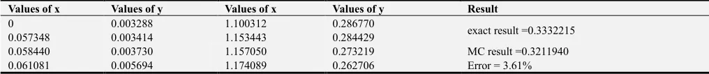
Table 1. Results and errors of the problem W : .
Values of x Values of y Values of x Values of y Result
0 0.003288 1.100312 0.286770
exact result =0.3332215
0.057348 0.003414 1.153443 0.284429
0.058440 0.003730 1.157050 0.273219 MC result =0.3211940
Error = 3.61%
Values of x Values of y Values of x Values of y Result
0.075477 0.029105 ……….. ……….
Trap result=0.3333936 Error = 0.05%
……….. ………. ………. ……….
……….. ………. ……….. ...
0.455328 0.192670 1.878003 0.0046863 simp13 result =0.3332478
Error = 0.007%
0.460976 0.194248 1.926177 0.0029224
0.463188 0.202385 1.959496 0.0020738
simp38 result =0.3343752 Error = 0.34%
0.474567 0.206180 1.975964 0.0017416
……….. ……… 2 0.0013418
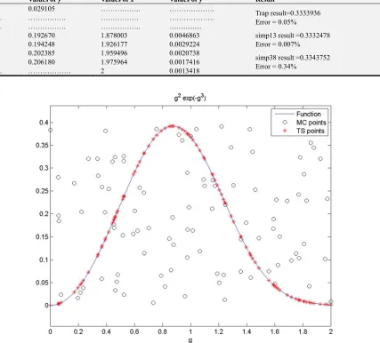
Figure 1. Graph of W : with random points.
4.2. Example 2
Consider the integration +R
We consider 100 random points over the intervals
Table 2. Results and errors of the problem +R .
Values of x Values of y Values of x Values of y Result
3 0.833333 3.97262038 0.2981448 exact result =0.6993584
3.00666912 0.825427 3.97436700 0.2977249 MC result =0.7794000
3.03720528 0.790700 4.02266877 0.2864654 Error = 11.44%
3.07440306 0.751424 4.04444260 0.2816025 Trap result=0.6970541
3.07802738 0.747763 ... ……… Error = 0.33%
……….. ……… ... ……… simp13 result =0.6972282
………... ………….. 4.94318550 0.154900 Error = 0.30%
simp38 result =0.7100770
3.33141259 0.54761197 4.94764765 0.154502 Error= 1.53%
3.33325416 0.54647726 4.96784356 0.15274 6
3.38405604 0.51656622 4.98607434 0.151131
3.39603472 0.50988508 5 0.150000
3.40014922 0.50762125
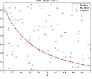
Figure 2. Graph of with random points.
4.3. Example 3
Consider the Heat equation4 XX5Y5 XYXZ, 0 30, [ \ 0. boundary conditions are [6, 7]
] 0, [ ] 30, [ 0, ] , 0 30 &
20 .
The Solution of the above equation is] , [ ∑`E _ sin d
+ cos
dZ + .
Here, _ + + + ∗ sin +d . We want to calculate _ using our above methods. We consider 200 random points over the interval 0, 30 and get the following results
Table 3. Results and errors of the problem + + + ∗ hi +d .
j Exact (
k
j) Trapezoidal TrapezoidalError (%) Simpson’s 1/3
Simpson’s 1/3 Error
(%) Simpson’s 3/8
Simpson’s 3/8 Error (%)
1 0.95493 0.954 0.09 0.830 13.08 0.773 19.05
2 0.477465 0.477 0.09 0.332 30.46 0.380 20.41
3 0.31831 0.3121 1.95 0.202 36.53 0.185 41.88
4 0.238732 0.2323 2.62 0.151 36.74 0.143 40.10
5 0.190986 0.1914 0.21 0.183 4.18 0.161 15.70
Again, we consider 500 random points over the interval 0, 30 and get the following results
Table 4. Results and errors of the problem + + + ∗ hi +d .
j Exact kj Trapezoidal Trapezoidal Error (%) Simpson’s 1/3 Simpson’s 1/3 Error (%) Simpson’s 3/8 Simpson’s 3/8 Error (%)
1 0.95493 0.9549 0.003 0.9486 0.66 0.9894 3.60
2 0.477465 0.4774 0.01 0.4728 0.97 0.4569 4.30
3 0.31831 0.3182 0.03 0.3133 1.57 0.3228 1.41
4 0.238732 0.2386 0.05 0.2358 1.22 0.2308 3.33
5 0.190986 0.1908 0.09 0.1869 2.17 0.1906 0.21
In our first two examples we see that choosing 100 points we find better approximation using our methods comparing to the well-known Monte- Carlo results using the same
observe that Simpson’s 1/3 rule gives better approximation than the other methods we have discussed.
5. Conclusion
The main objectives of this paper are to develop and understand solving numerical integration for the unequal data space by different methods with their errors. Firstly we derive the methods with their errors and then we use these methods to solve the numerical examples using computer program (MATLAB software) and we get sufficient accuracy comparing to the exact solution and Monte Carlo integration of the problems.
References
[1] Atkinson, K. E., 1978, An Introduction to Numerical Analysis, John Wiley & Sons, New York.
[2] Conte, S. D., 1965, Elementary Numerical Analysis, McGraw Hill, New York.
[3] Douglas Fairs, J., & L. Richard Burden, 2001, Numerical Analysis, Thomson Learning.
[4] Sastry, S. S., 2005, Introductory Methods of Numerical Analysis, Prentice-Hall of India.
[5] Ridgway Scott, L., 2011, Numerical Analysis, Princeton University press.
[6] Curtis F. Gerald, Patrick O. Wheatley, 2004, Applied Numerical Analysis, Pearson Education, Inc.
[7] William E. Boyce, Richard C. Diprima, 2001, Elementary Differential Equations and Boundary Value Problems, John Willey & Sons. Inc.
[8] Ward Cheney, David Kincaid, 2008, Numerical Mathematics and Computing, Thomson Brooks/Cole.
[9] F. B. Hildebrand, 1974, Introduction to Numerical Analysis, McGraw-Hill Book Company Inc.