http://www.sciencepublishinggroup.com/j/ajam doi: 10.11648/j.ajam.20180602.14
ISSN: 2330-0043 (Print); ISSN: 2330-006X (Online)
Comprehensive Evaluation of Logistics Enterprise
Performance Based on DEA and Inverted DEA Model
Zhang Qian, Zhang Bing-jiang
School of Applied Science, Beijing Information Science and Technology University, Beijing, China
Email address:
To cite this article:
Zhang Qian, Zhang Bing-jiang. Comprehensive Evaluation of Logistics Enterprise Performance Based on DEA and Inverted DEA Model. American Journal of Applied Mathematics. Vol. 6, No. 2, 2018, pp. 48-54. doi: 10.11648/j.ajam.20180602.14
Received: January 31, 2018; Accepted: February 13, 2018; Published: April 27, 2018
Abstract:
DEA is a systematic method for analyzing the relative effectiveness or benefit of decision- making units based on multi-index inputs and multi-index outputs, while Inverted DEA is a method for evaluating decision-making units based on ineffectiveness. In order to make a more reasonable evaluation of the decision-making unit, we consider using the characteristics of both DEA and Inverted DEA models to make a comprehensive evaluation of decision-making units. After discussing DEA model, Inverted DEA model and the comprehensive evaluation methods such as TOPSIS, a weighted geometric evaluation method was proposed. By using the proposed weighted geometric evaluation method and the other four evaluation methods, we evaluated the performance of 16 logistics enterprises in our country and the evaluation results were compared and sorted. The results show that the weighted geometric evaluation method can provide a new idea for the comprehensive evaluation based on DEA and Inverted DEA models.Keywords:
DEA, Inverted DEA, TOPSIS, Weighted Geometric Mean, Logistics Evaluation1. Introduction
Data Envelopment Analysis (DEA), first introduced by Charnes et al. in 1978, is used to evaluate the relative effectiveness of decision making units (DMUs) with multiple inputs and multiple outputs [1]. It uses mathematic programming models to create efficient frontier of production with well-evaluated DMUs, those DMUs that are not on the frontier will be compared with their peers on the frontier to estimate their efficiency scores.
The DEA evaluation method has the following characteristics: It is not affected by dimensions of input and output; the data of different indexes can be evaluated by a comprehensive index; the weight of the model is not affected by the subjective factors and the evaluation of the DMU is relatively fair; improvements can be proposed to inefficient DMUs; It has the absolute advantage of dealing with multiple inputs, especially multiple outputs. These obvious features make the DEA method develop rapidly in both theoretical research and practical application. Nowadays, DEA has been widely applied to management, systems engineering and decision analysis. For example, Shi et al. Proposed the application of DEA in decision support system [2], Mardani
et al. used DEA in energy efficiency [3].
However, in terms of DEA method, there are still some theoretical and practical problems. For example, during practical application, we found that it is probable to get more than one effective DMUs when we use DEA to evaluate the efficiency of DMUs. This has led to a lack of clear distinctions between evaluations and explicitly conclusive information is difficult to obtained, so that there is no practical help to decision-maker. To solve this problem, Allen et al. studied the weight constraints and value judgments in DEA in 1977 [4]. Andersen and Petersen (1993) improved the DEA model and proposed a more efficient way to evaluate the effectiveness of DMUs [5]. However, Banker and Chang pointed out in 2006 that the performance of super-efficient programs proposed by Andersen and Petersen did not perform well [6].
Yamada Yasuhito in 1994 [7], It is diametrically opposed to the concept of efficiency that DEA evaluates the effectiveness of DMUs, Inverted DEA is a model used to evaluate the anti-efficiency of DMUs. Because the traditional DEA model does not evaluate the DMU sufficiently, we consider introducing a combination of DEA and Inverted DEA to make a comprehensive evaluation of the DMU.
The Technique for Order Preference by Similarity to Ideal Solution (TOPSIS) was first proposed by HWang and Yoon in 1981 [8]. TOPSIS method is based on sort by the proximity of a limited number of objects to the ideal solution, and is a method of evaluating the relative merits of existing objects [9]. In fact, it is also a method of evaluating DMUs considering both the optimal solution and the worst solution. Based on the idea of TOPSIS, combined with the concepts of efficient value and anti-efficient value of DEA and Inverted DEA, a new DMU comprehensive evaluation method is proposed in this paper, which together with other evaluation methods, carrying out a comprehensive evaluation of the performance of 16 logistics enterprises in China.
2. DEA and Inverted DEA Models
2.1. DEA Model
The DEA model was first introduced by Charnes, Cooper, and Rhodes in 1978 called the C2R Model. There are n DMUs, each DMU has m inputs and s outputs.
Let
1 2
( , , , ) , 1, 2, ,
= ⋯ T = ⋯
j j j mj
X x x x j n
1 2
( , , , ) , 1, 2, ,
= ⋯ T = ⋯
j j j sj
Y y y y j n
be the jth input and output vectors of m and s dimension respectively, where,
0, 0, ( 1, 2, , ; 1, 2, , )
> > = ⋯ = ⋯
ij ij
x y i m r s
represent the ith type of input and the
r
th type of output of the j th DMU, which can be obtained from the observed sample data.The efficiency of the j0th DMU can be evaluated. The equivalent linear programming model of C2R is
0 0
0 max
s.t. 0, 1, 2, ,
1 0, 0 = − ≥ = = ≥ ≥ ⋯ T j j T T j j T j H Y
X Y j n
X µ ω µ ω ω µ (1)
where T =
(
1, 2,⋯,)
, T =(
1, 2,⋯,)
m s
ω
ω ω
ω
µ
µ µ
µ
are weightvectors of input and output respectively. By the duality principle of linear programming, the equivalent duality model of C2R is obtained.
0 0 min
s.t. , 1, 2, , , 1, 2, , 0, 0, ≤ = ≥ = ≥ ≠ ∈ ⋯ ⋯ T j j T j j n
X X j n
Y Y j n
E θ λ θ λ λ λ θ (2)
If we wish to measure the slacks of inputs and outputs, we can simply introduce some variables s+, s -as follows.
1 1
1
1
min ( )
s.t. , 1, 2, ,
, 1, 2, ,
0, 1, 2, ,
0, 0, 1, 2, , , 1, 2, ,
s m
r i
r i
n
j ij i ik j
n
j rj r rk j
j
r i
s s
x s x i m
y s y r s
j n
s s r s i m
+ − = = − = + = + − − + + = = − = = ≥ = ≥ ≥ = =
∑
∑
∑
∑
⋯ ⋯ ⋯ ⋯ ⋯ θ ε λ θ λ λ (3)where +=( 1+, 2+,⋯, +)
s
s s s s and −=( 1−, 2−,⋯, −)
m
s s s s are the slack
variables corresponding to the output and the input respectively, and ε is the infinitesimal non-Archimedean variable.
Let the optimal solution of linear programming be
λ
0,s−0,0 +
s ,
θ
0, and then we have(1) If
θ
0=1and s+≠0ors−≠0, DMUj0 is weak DEAefficient. That is, the j0 th DMU can obtain the same output by
reducing the input index or may increase the output when its inputs the same;
(2) If
θ
0=1ands+=s−=0, DMU is DEA efficient. That is, on the basis ofminput indexes of the j0th DMU, soutput indexes reach the optimum;(3) If
θ
0<1, DMUj0 is non-DEA efficient. That is the j0 thDMU can reduce the input index to obtain the same output
0
j
y .
2.2. Inverted DEA Model
Compared to the standard DEA models which evaluate DUMs from the perspective of optimism, Inverted DEA model is to evaluate the performance of DMUs from the perspective of pessimism.
To make an anti-efficiency evaluation of j0th DMU 0
(1≤ ≤j n) , we can use the Inverted DEA linear
programming model.
0 0
0 max
s.t. 0, 1, 2, ,
1 0, 0 ′ = ′ ′ − ′ ≤ = ′ = ′≥ ′≥ ⋯ T j j T T j j T j H X
X Y j n
where H′j0 represents the anti-efficiency value of j0 th
DMU,
ω
′T =(ω ω
1′ ′, 2,⋯,ω
m′) andµ
′T =(µ µ
1′ ′, 2,⋯,µ
′s) areweight vectors of input and output respectively.
By the duality principle of linear programming, the equivalent duality model of model (4) is obtained.
0 0 min
s.t. , 1, 2, ,
, 1, 2, , 0, 0
′
′ ≤ ′ =
′ ≥ =
′≥ ′≠
⋯
⋯
T
j j T
j j
Y Y j n
X X j n
θ
λ θ
λ
λ λ
(5)
where θ′represents the anti-efficiency value of j0 th DMU.
Introducing slack variables s′+ , s′− and infinitesimal non-Archimedes, model (4) is equivalent to the following.
1 1
0 1
0 1
min ( )
s.t. , 1, 2, ,
, 1, 2, , 0, 1, 2, ,
0, 0, 1, 2, , , 1, 2, , + −
= = + =
− =
+ −
′ − +
′ +′ = ′ = ′ −′ = = ′ ≥ =
′ ≥ ′ ≥ = =
∑
∑
∑
∑
⋯
⋯
⋯
⋯ ⋯
s m
r i
r i
n
j rj r r
j
n
j ij i i
j
j
r i
s s
y s y r s
x s x i s
j n
s s r s i m θ ε
λ θ
λ λ
(6)
where ′+=( 1′ ′+, 2+,⋯, ′+)
s
s s s s and ′−=( 1′ ′−, 2−,⋯, ′−)
m
s s s s are
the slack variables corresponding to the output and input, ε is infinitesimal non-Archimedes variable.
The optimal solution of model (6) is called Inverted DEA non-efficiency value, which represents inefficient measures of DMU. Inverted DEA non-efficiency means that θ′ =1 and
0, 0, 1, 2, , , 1, 2, ,
+ −
′ = ′ = = ⋯ = ⋯
r i
s s r s i m , while Inverted
DEA efficiency means θ′ <1 and s′ >r+ 0 or si′ >− 0 1, 2, , , 1, 2, ,
= ⋯ = ⋯
r s i m.
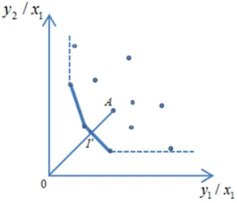
The standard DEA model is to evaluate the performance of DMUs from the performance of optimism, and on the contrary, Inverted DEA is to evaluate the performance of DMUs from the perspective of pessimism. Figure 1 and Figure 2 are the DEA efficiency diagram and the Inverted DEA anti-efficiency diagram respectively.
Figure 1. The DEA efficiency diagram.
Figure 2. The Inverted DEA anti-efficiency diagram.
3. Comprehensive Evaluation Methods
Based on DEA and Inverted DEA
Model
3.1. Mixed Synthesis Method
It’s clear that by utilizing the anti-efficiency value, we can obtain more information about performance and make the evaluation more reasonable. Therefore we consider aggregating the efficiency scoreθandθ′of DEA and Inverted DEA.
First we define the two indexes as the following.
* ( , )′ '* ( , )′
θ = θ θ ,θ = θ θ
For
θ
*, when we evaluate the performance of DMU1 andDMU2, we would compare the θ first, if θ > θ1 2 , the
DMU1 is considered performing better than DMU2, if θ = θ1 2,
than we continue to use θ′ to compare DMU1 and DMU2, if
1′ 2′
θ < θ , then DMU1 performs better than DMU2, while the
rank of θ'* is the opposite. This method uses the efficiency value and the anti-efficiency value to rank DMUs directly and make a comprehensive evaluation from the perspectives of efficiency and anti- efficiency respectively.
Liu put forward a synthetic evaluation index in 2007 [10] as follow.
1 1
2
+ − ′
= h
θ
θ
Because the ranges of θ and θ′ are different, it may not be a good idea to take the arithmetic average of the two indexes directly. So to keep the same orientation as θ, theθ′ should be transformed to 1 1− θ′. In this case, if DMU is anti- efficiency, θ′=1, h= θ ≤′2 1 2; if DMU is both efficiency and anti-efficiency, θ′=1,θ=1, h 1 2= ;if DMU is efficiency,
=1
This method unifies the range of θ and θ′, then take the average of them, which is easy to calculate and the use of information is also more adequate. However, the arithmetic mean is susceptible to extreme values, and if the data is obviously skewed, the representation of the arithmetic mean will be poor.
3.2. TOPSIS Method
TOPSIS method is a common method for multi-objective decision analysis of finite solutions in system engineering. Its basic idea is to define the ideal solution and negative ideal solution in decision problem, and then find a solution in the feasible solution, which is the closest to the ideal solution and the farthest from the negative ideal solution.
The steps of TOPSIS can be summarized as follow: Step 1 Normalize the decision matrix X.
2
1
1, 2, , ; 1, 2, ,
=
= = =
∑
⋯ ⋯
, ij ij n
ij i
X
a i n j m
X
than a normalized matrix A is obtained.
11 12 1
21 22 2
1 2 =
⋯
⋯
⋮ ⋮ ⋯ ⋮
⋯
m
m
n n nm
a a a
a a a
A
a a a
Step 2 Determine the ideal solution and negative ideal solution. The optimal value vector and the worst value vector are obtained according to the decision matrix A, That is, the optimal solution and the worst solution in the limited solution are:
1, 2, , {max 1, 2, , }
+=( + +⋯ +)= = ⋯
i i im ij
i
A a a a a j m
1 , 2 , , {min 1, 2, , }
−=( − −⋯ −)= = ⋯
i i i m ij
i
A a a a a j m
Step 3 Calculate the distance Di+ between each scheme and the ideal point and the distance Di− to the negative ideal point.
2
1
+ +
=
=
∑
( − )m
i ij ij
j
D a a
2
1
− −
=
=
∑
( − )m
i ij ij
j
D a a
where Di+ and Di− represent the distance between the i th evaluation object and the optimal solution and the worst
solution respectively, aij is the value of the j th index of the evaluation object i.
Step 4 Calculate the proximity Ci of the evaluation object and the optimal solution.
+ −
= +
-i i
i i
D C
D D
where Ci is between 0 and 1, the closer it is to 1, the closer it is to the optimal level. Conversely, the closer it is to 0, the closer it is to the poorest level.
Step 5 Sort by the relative proximityCiof each scheme. The value of Ciis larger, the overall benefit is better.
Among the many evaluation methods, the TOPSIS method is the most fully utilized information of the original data, and the result can accurately reflect the difference between the evaluation schemes. TOPSIS has no strict limits on the data distribution, the sample content and the index, and the data calculation is also simple. It is not only for a small sample, but also for multiple evaluation targets, multiple indicators of large sample data. Using the TOPSIS method for
comprehensive evaluation, we can draw a good
comparability to evaluate the ranking results.
4. Case Study Based on 16 Logistics
Enterprises Performance
4.1. Sample Data Source and Index Selection
Based on DEA and Inverted DEA models, this paper evaluates the performance of 16 major logistics enterprises in China through different evaluation methods. The evaluation data are from the annual reports of listed companies from 2006 to 2015, the average of the raw data of which was shown in Table 1.
As DEA efficiency is a relative efficiency, as long as each DUM is comparable, the calculation results are credible and able to truly reflect the efficiency of the indicators. In view of this, this article selected 16 logistics enterprises as the research object, the investment indicators are the total assets of I1 (ten
thousand yuan) operating costs I2 (ten thousand yuan), output
indicators are the main business income O1 (ten thousand
yuan), net profit O2 (ten thousand yuan) and earnings per share
O3 (yuan). The 16 logistics companies are Jinzhou
Port(DMU1), Dalian Port(DMU2), Beibu Gulf port (DMU3),
Lianyungang(DMU4), Nanjing Port(DMU5), Rizhao
Port(DMU6), Shanghai Port Group(DMU7), Shanghai
Lingang(DMU8), Tianjin Port(DMU9), Xiamen Port(DMU10),
Yantian Port(DMU11), Xiamen Airport(DMU12), Yingkou
Port(DMU13), Chongqing Port(DMU14), Tie Long
Logistics(DMU15), and Guangzhou-Shenzhen
Table 1. The average of the original data of 16 logistics enterprises from 2006 to 2015.
logistics enterprises I1 I2 O1 O2 O3
DMU1 862648 72404 114885 16444 0.10
DMU2 2233316 281874 397056 66578 0.20
DMU3 353705 109107 145138 16714 -0.39
DMU4 395017 86433 11962 10631 0.27
DMU5 87111 8522 14983 2299 0.13
DMU6 1069588 225322 311463 47361 0.40
DMU7 7457931 1261501 2123327 575425 0.14
DMU8 140942 78180 98433 1191 0.03
DMU9 2275617 936085 1185741 116836 0.36
DMU10 357664 286467 318685 20425 0.32
DMU11 533876 17489 41417 54005 0.57
DMU12 357664 41350 88202 31331 0.42
DMU13 1114830 164710 248793 34401 0.64
DMU14 438748 77741 105066 7831 0.15
DMU15 427047 239496 298462 35464 0.30
DMU16 3010460 953266 1234013 122260 0.17
4.2. Analysis of the Performance of Logistics Enterprises Based on Different Evaluation Methods
According to the input-output data of the 16 logistics enterprises in Table 1 and the model (3) and the model (6), we
obtains the relative efficiency value and the inefficiency value of the corresponding decision unit. Then the decision unit is evaluated with the four methods given in the previous article, and we sort the results. The ranking results are shown in Table 2.
Table 2. Ranking of Logistics Company Performance.
DMU θ Rank1 θ ′ Rank2 h Rank3 C Rank4
1 0.73 14 1.00 15 0.37 3 0.50 14
2 0.69 15 0.69 10 0.12 8 0.51 10
3 0.92 8 0.49 4 -0.07 12 0.51 5
4 0.27 16 1.00 16 0.14 7 0.51 7
5 0.82 11 0.74 11 0.24 5 0.50 12
6 0.85 10 0.50 5 -0.08 13 0.51 4
7 0.95 7 0.30 2 -0.68 15 0.51 2
8 1.00 5 1.00 14 0.50 1 0.00 16
9 0.95 6 0.55 8 0.07 9 0.51 9
10 1.00 4 0.77 12 0.35 4 0.50 13
11 1.00 2 0.39 3 -0.28 14 0.51 3
12 1.00 1 0.28 1 -0.82 16 0.51 1
13 0.80 12 0.66 9 0.14 6 0.51 11
14 0.77 13 0.98 13 0.37 2 0.50 15
15 1.00 3 0.51 6 0.02 11 0.51 6
16 0.90 9 0.54 7 0.02 10 0.51 8
According to the rank results in Table 2, we conduct a comprehensive analysis of the performance of 16 logistics enterprises. First of all, based on the relative efficiency and anti-efficiency values calculated by DEA and Inverted DEA, we obtain that the relative efficiency values of logistics enterprises 8, 10, 11, 12 and 15 are all equal to 1, indicating that these enterprises are effective for DEA. Enterprise 1, 4, 8 anti-efficiency value is 1, indicating that these three enterprises is anti-efficiency for Inverted DEA. Then we find that Rank1 and Rank2 are not much different in rankings, and Enterprise 4, 5, 12, and 14 are the same in the both rankings. While for enterprise 12, Rank 1, Rank 2, and Rank 4 are both 1 and Rank 3 is 16. We speculate that firm 12 performs best, and Rank 3 may be negatively correlated with other approaches.
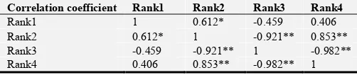
Next we conduct a correlation analysis of the four sorts:
Table 3. Correlation analysis of the four sorting methods.
Correlation coefficient Rank1 Rank2 Rank3 Rank4
Rank1 1 0.612* -0.459 0.406 Rank2 0.612* 1 -0.921** 0.853** Rank3 -0.459 -0.921** 1 -0.982** Rank4 0.406 0.853** -0.982** 1 **. The correlation is significant at the 0.01 level
*. The correlation is significant at the 0.05 level
5. Weighted Geometric Synthesis
Evaluation Method
5.1. Construction of Weighted Geometry Synthetic Evaluation Method
The commonly used combination comprehensive
evaluation methods are arithmetic average method, geometric mean method and mixed synthesis method. Among them, geometric mean method is more comprehensive in considering the distribution of weights of objects under evaluation, while multiplication is more sensitive to the changes of smaller values and is suitable for dealing with our problems.
Here we consider geometry-weighted combinations of θ and θ′.
g=
′α
θ
θ (7)
According to DEA and Inverted DEA models, we can know that θ and θ′ are indicators of the efficiency of DMUs. When θ is close to 1, or θ′ is close to 0, its efficiency is good. Then we weight the two values geometrically.
Also considering increasing the distinction between the evaluation results so that the difference is more obvious and rank is more visualized, we think the g should reach the maximum variance. According to this condition we can obtain the weight α. To facilitate the calculation, we take the logarithm of the formula (7).
= ln =ln − ln ′
i gi i i
ϕ
θ α θ
Then we get the expression ofα by finding the best value of variance of ϕ, after that we bring data in the expression to calculate the value of the weight. After calculation, we can get the weight α=-0.334 in the case, which we bring into the formula (7) and calculate the new rank, as shown in Table 4.
Table 4. Rank based on geometric weighting method.
DMU g Rank5(g) DMU g Rank5(g)
1 0.732 8 9 0.778 4
2 0.610 15 10 0.914 2 3 0.726 10 11 0.730 9 4 0.269 16 12 0.650 13 5 0.741 6 13 0.695 11 6 0.670 12 14 0.767 5 7 0.634 14 15 0.798 3 8 1.000 1 16 0.735 7
5.2. Comparison and Analysis of Five Comprehensive Evaluation Methods
We compare the performance rank generated by the weighted geometric evaluation method with the four rankings obtained in the previous section and find the correlation between the five ranking methods as shown in Table 5 and Table 6 below
Table 5. Rank of Logistics Company Performance Evaluation.
DMU Rank1 Rank2 Rank3 Rank4 Rank5
1 14 15 3 16 8
2 15 10 8 12 15
3 8 4 12 5 10
4 16 16 7 15 16
5 11 11 5 11 6
6 10 5 13 8 12
7 7 2 15 3 14
8 5 14 1 13 1
9 6 8 9 6 4
10 4 12 4 10 2
11 2 3 14 2 9
12 1 1 16 1 13
13 12 9 6 9 11
14 13 13 2 14 5
15 3 6 11 4 3
16 9 7 10 7 7
Table 6. Correlation Analysis of Five Sort Methods. correlation
coefficient Rank1 Rank2 Rank3 Rank4 Rank5
Rank1 1 0.612* -0.459 0.406 0.406 Rank2 .612* 1 -.921** .853** -0.279 Rank3 -0.459 -0.921** 1 -0.982 0.512* Rank4 .768** .953** -.871** 1 -0.576** Rank5 0.406 -0.279 0.512* -0.576* 1 **. The correlation is significant at the 0.01 level
*. The correlation is significant at the 0.05 level
From Table 5, we can see that in Rank1, Rank2 and Rank4, the performance evaluation of DMU12 is very good, while in
Rank3 and Rank5, it is ranked 16 and 13 respectively. The ranking of DMU2, DMU4, DMU15 in Rank 1 and Rank 5 is the
same. Based on the correlation analysis in Table 6, we can know that the rank of newly constructed weighted geometric mean evaluation methods and ranks of Rank3 and Rank4 are significantly correlated respectively based on the levels of 0.05 and 0.01, while the ranks of Rank1 and Rank2 Not significantly related. Therefore, we think that the newly constructed weighted geometric evaluation method is a comprehensive evaluation method, which can provide a new idea for the evaluation based on DEA and Inverted DEA models.
6. Conclusion
Acknowledgements
The research was supported by the National Natural Science Foundation of China (Grant No. 60972115).
References
[1] Charnes, A., W. W. Cooper, and E. Rhodes. "Measuring the efficiency of decision making units." European Journal of Operational Research 2.6(1978):429-444.
[2] Shi, Ping, et al. "A decision support system to select suppliers for a sustainable supply chain based on a systematic DEA approach."Information Technology & Management 16.1(2015):39-49.
[3] Mardani, Abbas, et al. "A comprehensive review of data envelopment analysis (DEA) approach in energy efficiency." Renewable & Sustainable Energy Reviews 70. In press(2016):In press.
[4] R. Allen, et al. "Weights restrictions and value judgements in Data Envelopment Analysis: Evolution, development and future directions."Annals of Operations Research 73.1(1997):13-34.
[5] Andersen, Per, and N. C. Petersen. "A Procedure for Ranking Efficient Units in Data Envelopment Analysis." Management Science39. 10(1993):1261-1264.
[6] Rajiv D. Banker, and Hsihui Chang. "The super-efficiency procedure for outlier identification, not for ranking efficient units." European Journal of Operational Research 175.2(2006):1311-1320.
[7] Yamada, Yoshiyasu, T. Matsui, and M. Sugiyama. "AN INEFFICIENCY MEASUREMENT METHOD FOR MANAGEMENT SYSTEMS." Journal of the Operations
Research Society of Japan 37.2(1994):158-168.
[8] Hwang, C. L., and Yoon, K. "Multiple Attribute Decision Making: Methods and Applications." Springer-Verlag, New York.
[9] Tzeng, Gwo Hshiung, and J. J. Huang. "Multiple Attribute Decision Making: Methods and Applications." European Journal of Operational Research 4.4(2011):287-288.
[10] Liu, Wb, et al. "DEA Analysis Based on both Efficient and Anti-Efficient Frontiers." (2007).
[11] Guo, Cun Zhi, et al. "Construction of the Indexes of DEA Used in Comprehensive Evaluation of Sustainable Development." China Population Resources & Environment (2016).
[12] Shen, Wan Fang, et al. "Increasing discrimination of DEA evaluation by utilizing distances to anti-efficient frontiers." Computers & Operations Research 75. C(2016):163-173. [13] Carayannis, Elias G., E. Grigoroudis, and Y. Goletsis. "A
multilevel and multistage efficiency evaluation of innovation systems: A multiobjective DEA approach." Expert Systems with Applications 62(2016):63-80.
[14] Jin, Han Park, Y. K. Ji, and Y. C. Kwun. "Intuitionistic Fuzzy Optimized Weighted Geometric Bonferroni Means and Their Applications in Group Decision Making." Fundamenta Informaticae 144.3-4(2016):363-381.
[15] Emrouznejad, Ali, and G. L. Yang. "A survey and analysis of the first 40 years of scholarly literature in DEA: 1978–2016." Socio-Economic Planning Sciences (2017).