Enabling More Accurate and Efficient Structured Prediction

(1)

University of Pennsylvania

ScholarlyCommons

Publicly Accessible Penn Dissertations

1-1-2013

Enabling More Accurate and Efficient Structured

Prediction

David Joseph Weiss

University of Pennsylvania, [email protected]

Follow this and additional works at:http://repository.upenn.edu/edissertations Part of theComputer Sciences Commons

This paper is posted at ScholarlyCommons.http://repository.upenn.edu/edissertations/942

For more information, please [email protected]. Recommended Citation

(2)

Enabling More Accurate and Efficient Structured Prediction

Abstract

Machine learning practitioners often face a fundamental trade-off between expressiveness and computation time: on average, more accurate, expressive models tend to be more computationally intensive both at training and test time. While this trade-off is always applicable, it is acutely present in the setting of structured

prediction, where the joint prediction of multiple output variables often creates two primary, inter-related bottlenecks: inference and feature computation time.

In this thesis, we address this trade-off at test-time by presenting frameworks that enable more accurate and efficient structured prediction by addressing each of the bottlenecks specifically. First, we develop a

framework based on a cascade of models, where the goal is to control test-time complexity even as features are added that increase inference time (even exponentially). We call this framework Structured Prediction Cascades (SPC); we develop SPC in the context of exact inference and then extend the framework to handle the approximate case. Next, we develop a framework for the setting where the feature computation is explicitly the bottleneck, in which we learn to selectively evaluate features within an instance of the mode. This second framework is referred to as Dynamic Structured Model Selection (DMS), and is once again developed for a simpler, restricted model before being extended to handle a much more complex setting. For both cases, we evaluate our methods on several benchmark datasets, and we find that it is possible to dramatically improve the efficiency and accuracy of structured prediction.

Degree Type

Dissertation

Degree Name

Doctor of Philosophy (PhD)

Graduate Group

Computer and Information Science

First Advisor

Ben Taskar

Keywords

computer vision, machine learning, natural language processing, structured prediction

Subject Categories

(3)

ENABLING MORE ACCURATE AND EFFICIENT STRUCTURED PREDICTION

David Weiss

A DISSERTATION

in

Computer and Information Science

Presented to the Faculties of the University of Pennsylvania

in

Partial Fulfillment of the Requirements for the

Degree of Doctor of Philosophy

2013

Supervisor of Dissertation Ben Taskar

Associate Professor, Computer and Information Science Graduate Group Chairperson

Val Tannen, Professor, Computer and Information Science Dissertation Committee:

Kostas Daniilidis, Professor, Computer and Information Science Daniel Lee, Professor, Computer and Information Science

(4)

ENABLING MORE ACCURATE AND EFFICIENT STRUCTURED PREDICTION

COPYRIGHT

2013

(5)

(6)

Acknowledgements

I would like to first thank and acknowledge my advisor, Ben Taskar. This thesis would simply not exist without his unwavering expert guidance, encouragement, and support. His boundless energy and enthusiasm for our work pushed me to achieve what I thought was impossible. I could not have asked for a better advisor.

I am grateful to Kostas Daniliidis, the chair of my committee, for his consistent advice and confidence in me. I would also like to thank the rest of my committee–Dan Lee, CJ Taylor, and Pedro Felzenszwalb–for helping me forge my years of effort into a single coherent document. I am also indebted to my original co-advisor Michael Kearns, who shaped the start of my time in graduate school.

During my time at Penn, I was fortunate to be surrounded by an amazing community of colleagues and friends. I count myself lucky to have had the opportunity to work so closely with Benjamin Sapp. Without Andrew King, I would have missed out on an amazing paper title and acronym. Many thanks to Alex, Alex, Cody, Chris, Christine, Emily, Joao, Jenny, Katie, Katerina, Kuzman, Matthieu, Ryan, Steve, and Umar. I would not have made it through this process without you.

(7)

ABSTRACT

ENABLING MORE ACCURATE AND EFFICIENT STRUCTURED PREDICTION David Weiss

Ben Taskar

Machine learning practitioners often face a fundamental trade-off between expressiveness and computation time: on average, more accurate, expressive models tend to be more com-putationally intensive both at training and test time. While this trade-off is always applica-ble, it is acutely present in the setting ofstructured prediction, where the joint prediction of multiple output variables often creates two primary, inter-related bottlenecks: inference and feature computation time.

(8)

List of Tables

4.1 Summary of key notation. . . 33

4.2 Summary of WSJ results . . . 45

4.3 Summary of handwriting recognition results . . . 47

(12)

List of Illustrations

3.1 Several common factor graphs . . . 22

3.2 Agglomerating variable states . . . 24

3.3 Removing loops from a trigram model . . . 26

4.1 High level overview of SPC framework . . . 31

4.2 Sample cascade output . . . 32

4.3 Computing max-marginals . . . 34

4.4 Thresholing bigrams using max-marginals . . . 35

4.5 Sparsity of inference . . . 43

5.1 Example tree decomposition . . . 50

5.2 Schematic overview of Ensemble-SPC . . . 55

5.3 Synthetic segmentation results . . . 56

5.4 Qualitative Ensemble-SPC test results . . . 58

5.5 Prediction error on videopose dataset . . . 60

6.1 Trade-off on handwriting recognition task . . . 66

6.2 MODEC+S exceeds state-of-the-art . . . 68

6.3 Dynamic model selection on the CLIC dataset . . . 71

6.4 Expansion distribution of DMS . . . 77

6.5 Qualitative results on CLIC dataset . . . 78

(13)

(14)

Chapter 1 Introduction

This thesis is motivated by the inherent trade-off in applied machine learning of expressive-nessvs. computation. To make this concrete, we consider supervised discrete prediction problems where the goals is to predict a discrete output variableY given some input X.

Specifically, we assume we have a linear hypothesis of the form:

h(x) = argmax y∈Y

w>f(x,y) (1.1)

whereY is the domain ofY (the output space), wis a parameter weight vector andf is a

feature generating function. This linear prediction framework encompasses most standard supervised learning settings and algorithms, where the goal is to learn a parameter vector

win order to minimize some expected error for a prediction task in a given domain.

In this thesis, we are instead primarily concerned with the question: what are the com-putational requirements of evaluating h(x)? As an example, consider an instance of the standard multi-class classification problem from computer vision is image classification, wherexis an input image,_Y =_{1, . . . , K_}(whereK is the number of classes of images),

(15)

bottle-neck, then the expressiveness vs. computation trade-off is intuitively very simple: adding more features to the model increases the expressiveness of the model at additional compu-tational cost.

Given a set of models of varying expressiveness and computational cost, the standard staticmodel selectionproblem is to choose a model that which is closest to a given target in the space of possible trade-offs. For example, we might desire the most accurate face detector that runs in less than a fraction of a second on a typical server, or we might desire the most efficient face detector that still achieves 99.9% recall on a standard benchmark. To make the example still more concrete, suppose we have a hierarchy of feature generat-ing functionsf1 ⊆ f2. . .fD, each requiring more time to compute than the previous. One simple model selection technique would be to learn parameter vectorsw1, . . . ,wD sepa-rately for each model using standard machine learning techniques, evaluate each one on a development data set, and choose the one that best satisfies our problem constraints using estimates of runtime and accuracy on the development set.

In contrast, in this thesis we study test-time model selection methods that, given a model hierarchy, can achieve a much more accurate hybrid model with the same or better expected runtime as the static model selection scheme just described. For example, the highly influential classifier cascade of Viola and Jones (2002) provided a significant leap in state-of-the-art performance for face detection. At a high level, the classifier cascade approach to model selection is use a hybrid model that utilizes the cheapest model fj in

f1, . . . ,fD that has marginwj>fj(x,y)above some threshold; in this way, “easy” examples

will be evaluated quickly while “hard” examples will be assigned more computation time; on average, the accuracy can reach that of the most expensive model, while the computation time remains much lower. The contributions of this thesis can best be understood within the space of multi-stage, hybrid model selection techniques.

(16)

features are computed. Put simply, structured prediction is the joint prediction of multi-ple discretely-valued output variables, and this problem arises in many application areas of machine learning. For example, one problem studied in this thesis is handwriting recogni-tion, or the joint prediction of the English letters associated with a sequence of handwritten characters. Note that this problem still falls in the general framework forh(x)from (1.1); for a sequence of length`and an alphabet of sizeK, we simply have that_Y is the product

of ` discrete spaces _{1, . . . , K_}. The key empirical finding is that structured prediction–

making predictions for each character simultaneously–provides far more accurate results on this task than the alternative of making separate predictions for each character indepen-dently. The reason that the data isnotgenerated independently for each character: because the writer is writing English words, the assignment of each letter in the word carries infor-mation on nearby letters.

Structured prediction is a natural framework both for learning high-order statistics of the data, and for incorporating hard constraints on the output space. By explicitly represent-ing such interactions as features, structured prediction allows one to learn the higher-order statistics of the training data, and thereby ensure that predictions properly take into account interactions between output variables at test time. Furthermore, in certain settings, there exist hard constraints on the interactions between output variables: for instance, in natu-ral language processing, producing a dependency parse of a sentence requires predicting a parent-child relationship for each word such that the resulting directed graph is a tree.

As might be expected, the additional expressiveness of structured prediction over inde-pendent predictions comes at an increased computational cost: becauseY is exponentially

large (|Y| = K`, as defined above), naively computing the argmax becomes practically

(17)

if we add triplets of neighboring characters, the complexity is O(`K3₎_{. Thus, for}

struc-tured prediction, the expressiveness-computation trade-off can be summarized as follows: introducing additional features increases expressiveness at the cost of increased feature computation time, but may additionally increase inference time, possibly to the point of making the problem infeasible.

1.1 Thesis Overview

The primary contribution of this thesis is to provide two different and complementary meth-ods for obtaining better expressiveness-computation trade-offs in the setting of structured prediction. The key to each of our approaches is tolearnto control the complexity of in-ference or feature computation at test time, on a per-example basis. As we will see, the first methods we discuss are meant to address the inference bottleneck; the next methods are meant to address the feature computation time bottleneck. Specifically, we outline the organization of this thesis as follows:

• Chapter 2 - Related work. In this chapter, we place the thesis in context by

re-viewing the relevant literature that either precedes or competes with our approaches; much of the ideas in this work stem from related work in multi-class classification, while we compete with alternative methods in the structured prediction community.

• Chapter 3 - Structured Prediction. We next provide a brief overview of the

key technical details of structured prediction, to provide a common foundation with which we can present and analyze the frameworks described in this thesis. Note that a complete tutorial is outside the scope of this thesis; see e.g. Nowozin and Lampert (2011) for a more complete tutorial. The purpose of this chapter is to provide enough background to understand the bottlenecks of inference and feature computation time that we address in this thesis.

• Chapter 4 - Structured Prediction Cascades (SPC). In the next chapter, we

(18)

Cascades (SPC). The goal of SPC is to progressively filter orprunethe output space such that sparse, exact inference remains feasible even when very complex features are added to the model. This chapter is based on the preliminary work (Weiss and Taskar, 2010).

• Chapter 5 - Ensemble-SPC. The major limitation of SPC is that it requires exact

inference to be feasible in every model in the cascade; thus, in the next chapter, we extend SPC to the setting where exact inference is intractable by usingensemblesof models. This chapter is based on preliminary work (Weiss et al., 2010).

• Chapter 6 - Dynamic structured model selection (DMS).We next turn to the

prob-lem of feature computation time. We propose a framework for selectively allocating resources across a batch of test examples by running a cascade of arbitrarily con-structed structured models. This is based on preliminary work (Weiss and Taskar, 2013).

• Chapter 7 - DMS-π. In this chapter, we revisit the feature extraction problem for

structured models and provide a more fine-grained formulation using principles from reinforcement learning. This allows us to selectively compute features within specific examples and learn a non-myopic feature extraction policy, which leads to large gains in efficiency over the original DMS approach. This is based on preliminary work under review at the NIPS2013 conference.

• Chapter 8 - Future work. Finally, we propose unifying the SPC and DMS-π

(19)

Chapter 2 Related Work

The basic expressiveness-computation trade-off has been studied in the machine learning literature in various settings and for a variety of reasons. In this section, we review the relevant literature and place this thesis in a broader context. As discussed previously, there is a significant amount of related work studying the expressiveness-computation tradeoff in multi-class classification. While many of the principles or high level ideas of the same–e.g., applying a cascade of models or using reinforcement learning to model feature extraction– applying these ideas to the structured case is not trivial, and many new insights are to be gained in the process. Thus, we first review the multi-class literature and then delve into related or competing approaches for structured prediction.

However, there are several themes that consistently arise in both the multi-class and structured setting. Generally speaking, we can categorize the related literature along several axes:

• Training time vs. test time. Much prior work has focused on model selection during

training–efficiently finding the most accurate fixed model with bounded complexity. In contrast, the contributions of this thesis allow for adaptive complexity chosen dynamically at test-time.

• Single- vs. multi-stage.One point of emphasis in prior work is limiting the

(20)

training or dynamically at test-time, for example by selectively computing a subset of the possible features to limit the cost. An alternative is to propose a multi-stage approach that makes a series of increasingly expensive decisions. In this case the depth of processing of a certain example determines the cost of evaluation. The work of this thesis spans both of these cases: in DMS-π, we selectively compute features in

a single structured model, while in SPC and DMS, we use a cascade of increasingly expensive models.

• Myopic vs. non-myopic.Both the work in this thesis and related approaches allocate

resources at test-time in an piecemeal fashion, repeatedly deciding whether or not more computation is necessary for a given example. One important property of such approaches is whether or not computation is allocated myopically, i.e. without a belief of how early steps in the computation will affect later outcomes. A typical approach to learning non-myopic strategies is to borrow techniques from the field of reinforcement learning, and that is the approach taken in this thesis for DMS-π in

Chapter 7.

• Implicit vs. explicit meta-level reasoning.One distinction of the work in this thesis

that has received far less prior attention is the idea of explicitmeta-levelreasoning: i.e. learning a distinct model with seperate meta-level features that can examine the current state of the predictive system and reason about how to proceed. For example, while our SPC framework is based around eliminating low-scoring outputs based on adaptive thresholds, the DMS/DMS-πframework explicitly learns a separate model

that evaluates the output of the structured predictor and computes values that guide further computation. Most prior work, on the other hand, falls into the implicit cate-gory.

(21)

2.1 Controlling computation of multi-class classification

The general ideas inspiring the particular methods proposed in this thesis are not new; in many cases, our intuition comes from prior work studying the computational trade-offs in the setting of multi-class classification. In many ways, one of the goals of this thesis is to translate ideas and advances from the multi-class case into the structured prediction setting. In what follows, we provide an overview of the themes from the flat classification literature that are related to or (in some cases) directly inspired the work of this thesis.

2.1.1 Computational trade-offs during model selection

Model selection has long been studied within the framework of empirical risk minimization (Bartlett et al., 2002; Vapnik and Chervonenkis, 1974), in which the primary criteria is the trade-off between approximation error (the bias of the model) and estimation error (overfitting, or the variance of the parameter estimates). For this case, model selection again consists of finding the most accurate model that falls within a complexity constraint. However, unlike the model selection considered in this thesis, the complexity measure is not defined with regards to computation. Rather, it is defined with respect to the expressive power of the model. The general intuition in this case is that as more data is obtained, the parameter estimates for more more expressive models become useful.

(22)

is available and computation time at training is limited, stochastic optimization methods should be used. Since our setting assumes both properties, we employ such such stochastic learning techniques in this thesis.

Both of these works assume a single fixed class of models, while in more recent theoret-ical work, Agarwal et al. (2011) propose methods for model selection under training time computational constraints when given a hierarchy of increasingly complex models. This problem is more similar to that addressed in this thesis, but, as above, Agarwal et al. (2011) study the problem of allocating computation time during training, with no constraints on fixed test-time computational costs.

2.1.2 Predicting with fixed test-time budgets

More directly related to the work in this thesis is prior work on explicitly controlling the fixed test-time cost of the model through regularization during training. These works at-tempt to answer the question: how do we efficiently learn an accurate model that has hard constraints on a fixed test-time cost? A popular approach is to express test-time com-plexity as convex regularization term that penalizes expensive models during training, for example learningsparse(Langford et al., 2009) orlow rank(Harchaoui et al., 2012) param-eter vectors. Sparse models use only subset of the features, and therefore certain features may not need to be computed; low rank models use an intermediate representation that is shared among different classes, speeding up the argmax problem for multi-class classifica-tion whenK is very large. However, while these works also seek to control test-time costs,

these approaches yield a single model of fixed computational cost for every test example. In contrast, the methods presented in this thesis learn models for expected run-time that compute different features for each different test-example.

(23)

evaluation cost, and a delay cost corresponding to the time taken to perform medical tests. More recently, Grubb and Bagnell (2012) propose a boosting algorithm designed to maxi-mize accuracy for any fixed test-time cost, while Xu et al. (2012) propose a boosting-type algorithm for learning ensembles of decision trees that explicitly trade-off computing new features vs. re-using already computed features in later stages of boosting.

Finally, another related area for controlling test-time complexity at training is in the domain of kernelized methods: kernelized models’ computational cost at test-time is de-termined primarily by the number ofsupport vectorsretained during training to implicitly parameterize the feature vector of the model. Learning kernelized models on a budget has been well studied in the on-line setting (Crammer et al., 2003; Dekel et al., 2008), where an active set of support vectors is maintained and updated as new examples are observed. However, we do not study kernelized models in this thesis, and therefore the notion of budget as number of support vectors is qualitatively different from the budget we define in terms of the cost of computing features.

2.1.3 Resource allocation for batch testing

(24)

2.1.4 Classifier cascades

A significant source of related work to the approaches proposed here is the study of clas-sifier cascades, in which a pre-determined series of classification models are sequentially applied to a test example. For binary classification problems with a highly skewed class distribution with very few true positives, these works typically obtain efficiency via an “early-exit” strategy: at test-time, simpler models may reject an example as negative with-out needing to evaluate the more complex models farther along the cascade. This approach has long been highly successful for object detection, using boosting methods to train the cascade of classifiers (Viola and Jones, 2002). Significant effort has been put into frame-works for jointly learning the classifiers of the cascade (Lefakis and Fleuret, 2010) or con-structing cascades automatically (Saberian and Vasconcelos, 2010). Feature computation cost was not incorporated specifically into the learning procedure until more recently. For example, Raykar et al. (2010) and Chen et al. (2012) propose training procedures for jointly training a cascade that explicitly represent a trade-off between accuracy and a measure of runtime complexity. These works inspired our SPC framework, which translates the idea of early-exit cascades into the structured setting.

2.1.5 More general multi-stage decision systems

There have been a number of more general formulations of a multi-stage classifier that expand on the idea of classifier cascades. For multi-class problems, the “early-exit” strategy for classifying negative examples does not apply directly, since there is no negative class. Instead, a more natural formulation is introduce an additional “reject” class to form a(K+ 1)-way classification problem; if a classifier predicts “reject,” the example is passed to the

next classifier (Trapeznikov and Saligrama, 2013). In this way, predicting anything besides “reject” can be seen as an early exit strategy.

(25)

classifiers and two additional components: one to estimate the confidence of the classifier and another to non-myopically determine a rejection threshold based on the confidence. If the classifier is not confident enough, then the “reject” action is taken for a given stage. The whole system is learned in an iterative stage-wise fashion. A similar approach is taken by Busa-Fekete et al. (2012), who assume that the series of classifiers is fixed a priori–learned via AdaBoost–and instead introduce an additional “skip” action that allows the system to short-circuit the decision process. Unlike Trapeznikov et al. (2013), Busa-Fekete et al. (2012) use standard reinforcement learning techniques to learn a policy to determine the actions taken at prediction time. While the models used in these frameworks differs greatly from the structured setting we study, we use similar principles from reinforcement learning to non-myopically learn a policy for feature extraction in our DMS-πframework.

Another multi-stage framework addressing a somewhat different problem than those just mentioned is closely related to SPC: This is thelabel treeframework for large multi-class tasks, first proposed by Bengio et al. (2010). A label tree is a decision tree where each decision node eliminates a fraction of the label space, such that at the leave nodes only comparison between a small number of classes is needed. At a high level, this idea is similar to that of SPC proposed in this thesis, except that instead of scoring, filtering, and maintaining a list of multiple overlapping partitions of the output space, the tree maintains and repeatedly filters only a single partition. However, Deng et al. (2011) show how the label tree can be explicitly optimized for accuracy and efficiency in a manner similar to the objectives posed for SPC. More recently, Liu et al. (2013) show how to learn probabilistic classifiers at each decision node to dramatically improve the performance of the tree; how-ever, this is significantly different from the non-probabilistic approach taken throughout this thesis.

2.1.6 Feature extraction policies

The idea of learning a feature extraction policy, as in our DMS-π framework, is not

(26)

of feature values, and the policy chooses individual features to evaluate. This generative setting differs greatly from the discriminative setting studied in this thesis; in the generative approach, one models a distributionP(f(X), Y)and uses Bayes rule to make predictions. One approach to feature extraction given a generative model is to maximize thevalue of in-formation, which is a measure of the information aboutP(Y _|f(X))gained by observing new features, subject to cost constraints. Though generally infeasible, approximations exist given graphical models of the data or for special cases (Bilgic and Getoor, 2007; Krause and Guestrin, 2005, 2009). The policies can also be learned using reinforcement learning techniques; e.g. Ji and Carin (2007) formulate the feature extraction problem as a Par-tially Observable MDP (POMDP) and use Gaussian Mixture Models (GMM) to model the features, while Bayer-Zubek (2004) use discrete distributions in a standard MDP frame-work. It’s noteworthy that in both cases, the best empirical policies are defined myopically, greedily optimizing a heuristic, despite formulating the problem using the standard rein-forcement learning frameworks.

There has been less work on discriminative approaches to feature extraction policies. Recently, several works have proposed modeling the value of a classifier in terms of the features used. For instance, Gao and Koller (2011) explicitly model the information gain of introducing additional features for a particular example, based on a pre-trained pool of classifiers that use different subsets of features; in this case, a GMM is used to model a joint distribution over possible classifier outputs and class labels, rather than modeling the features directly. Additionally, He et al. (2012)–who use an imitation learning approach for dynamic feature selection–avoid modeling a value function altogther and instead learn a classifier using meta-features of previous outputs in order to classify which feature subset to compute next. Note that although both of these approaches are similar in spirit to the reinforcement learning framework used for DMS-π, neither of these approaches apply to

(27)

2.2 Related approaches for structured prediction

In this next section, we review prior work that also attempts to solve the expressiveness-computation trade-off in the structured setting. These methods are more directly com-parable to our work than the literature discussed in the previous section, so we focus on highlighting the distinction between previous, related work and the work presented in this thesis.

2.2.1 Coarse-to-fine reasoning

The SPC framework proposed in this work can be considered as an instance of coarse-to-fine reasoning: as implemented in practice, early stages of the cascade eliminate outputs using a much coarser partitioning of the output space than the later stages. This basic idea has been used before in the structured setting, and we review some key examples here.

The simplest approach to coarse-to-fine reasoning is to use a two-step inference proce-dure: before running inference in a complex model, a simpler model computes marginals over the state space, and any states with low probability are eliminated. In natural lan-guage parsing, many works (e.g. Carreras et al. (2008); Charniak (2000)) utilize this idea: the marginals of a simple context free grammar or dependency model are used to prune the parse chart for a more complex grammar. The key difference with our work is that we explicitly learn a sequence of models tuned specifically to filter the space accurately and ef-fectively; furthermore, because we use discriminative max-marginals instead of probabilis-tic marginals, we can provide theoreprobabilis-tical bounds on the generalization error of our filtering steps. Somewhat closer to our work is that of Petrov (2009), where an entire hiearchy of coarse-to-fine grammars is learned; however, we do not learn the structure of the hierarchy of models but assume it is given by the designer, and again we use a different objective for learning the coarse-to-fine hierarchy and a different filtering scheme at test-time.

(28)

is trained to minimize expected computational cost. More recently, Pedersoli et al. (2011) use coarse-to-fine processing in the structured setting by utilizing the scores of parts in low-resolution object models to prune the search space over part locations in high-low-resolution models. Once again, however, our work proposes a different filtering scheme and a differ-ent learning objective–and most importantly, our filtering criterion integrates information from an entire structured model rather than using local scores to prune hypotheses.

Raphael (2001) provide a provably correct coarse-to-fine method for solving arbitrary dynamic programs. This approach relies on partitioning the full state space into “super-states,” and then efficiently computing upper and lower bounds on all possible transitions between the constituents within superstates; superstates can be eliminated from the search procedure once their bounds indicate the solution does not lie within. In a certain sense, the SPC approach proposed in this thesis substitutes efficiently computing bounds with efficiently computing max marginals, which is more useful in practice, but at the cost of potential sub-optimality if the learned filters are incorrect on a given example.

2.2.2 Early stopping cascade

(29)

2.2.3 Prioritized inference

While modeling the feature extraction process as an MDP has been studied in the multi-class setting, using reinforcement learning to speed-up evaluation of structured models has been less well studied. One significant prior work is Jiang et al. (2012), who apply imitation learning to speed up inference in a syntatic parsing model; however, the state of their MDP is defined solely in terms of the inference procedure and does not explore feature sets in any way. In contrast, the DMS-πframework we propose focuses on feature extraction as a

bottleneck, not inference as a bottleneck.

2.2.4 Meta-learners/predicting model accuracy

Another core component of the DMS/DMS-πapproach is the idea of using meta-features

to evaluate the progress of a structured model; this basic idea of predicting the accuracy of a model has been studied before, albeit in different contexts. E.g. Bedagkar-Gala and Shah (2010) attempt to predict various video analysis algorithm’s performance (similar in spirit to the selector we propose), but based on measures of image quality rather than properties of model output. Jammalamadaka et al. (2012) propose an evaluator for human pose estimators, but only for single-frame images, and propose only learning “correct or not” coarse-level distinctions, whereas we attempt to predict a measure of the error of each model directly. In the speech community, Lanchantin and Rodet (2010) propose a parallel method of “dynamic model selection” in which several models are continually re-evaluated in an online fashion using a generative model, which is a very different setting than that we analyze here.

2.2.5 Applications of preliminary works

(30)

ap-plied the SPC framework to human pose estimation in static images, using a coarse-to-fine multi-resolution framework similar to that used in section 5.5.2 of this thesis. Subsequent to Weiss et al. (2010), Sapp et al. (2011) applied the summation of max marginals from Ensemble-SPC in a different model of human pose in order to further advance state-of-the-art in pose tracking. However, in this work, we show how a sequence model built on the output of Sapp and Taskar (2013) yields faster, more accurate predictions, and we propose DMS to further speedup the evaluation of this model.

In natural language processing, Rush and Petrov (2012) apply the ideas developed in our preliminary work to the problem of dependency parsing in natural language processing. They learn a cascade of simplified parsing models using the objective presented in section 4.3 to achieve state-of-the-art performance in dependency parsing across several languages at about two orders of magnitude less time.

2.3 Summary

(31)

Chapter 3 Structured Prediction: An Overview

In this chapter, we provide a short tutorial and overview of the structured prediction meth-ods that form a basis for the work in this thesis. We also introduce notation and language that will be used throughout.

3.1 Supervised learning

Given an input space X, output space Y, and a training set{(x1_{, y}1₎_{, . . . ,}₍_xn_{, y}n₎_} _of _n samples from a joint distributionD(X, Y), the standard supervised learning task is to learn a hypothesis h : _{X 7→ Y} that minimizes the expected loss _ED[L(h(X), Y)] for some non-negative loss functionL :_{Y × Y →}_R+_{. This minimization is performed with respect}

to some hypothesis space H. For example, in the linear binary classification setting, we

typically haveY =_{−1,+1_}being the binary label,_L(Y, Y0) =1[Y ₆=Y0]being the 0-1 loss indicating whether or not a prediction is correct, and learn linear hypotheses of the formh(x) = sign(w>f(x)), where w_∈ _Rm _{parameterizes the model as a linear function} of a computed feature vectorf.

In practice, minimizing the expected error in this setting can be difficult for three rea-sons:

(32)

• We can only estimate the loss via the n samples of the training set, and minimize

with respect to this estimate.

• We may run out time trying to estimate the parameters forhor even computeh(x).

The standard solution to the first problem is to replace Lwith a convex upper bound; the choice of bound leads to different flavors of optimization problems. However, the second problem leads to a trade-off: as we increase the expressiveness of the model (as measured by the number of parametersm), we decrease the reliability of our estimate of the loss of

the minimizer h? _{for any fixed number of training samples} _n_{. In other words, we trade} off approximation error with estimation error; a simpler model may make mistakes due to approximatingD(X, Y)poorly, but a more complex model may make mistakes due to poorly estimatingw. This classical trade-off between approximation and estimation error

(bias/variance) is fundamental in machine learning and has been well studied. Standard sta-tistical model selection techniques (Akaike, 1974; Barron et al., 1999; Bartlett et al., 2002; Devroye et al., 1996; Vapnik and Chervonenkis, 1974) control this trade-off to minimize expected error by exploring a hierarchy of models of increasing complexity.

In this thesis, we are primarily concerned with the third final problem, which also yields a trade-off: as discussed in Chapter 1, increasing the expressiveness of the model also typically leads to increased computation time. In the next section, we make this problem concrete for the structured setting, and make explicit the two primary potential bottlenecks (inference and feature extraction). Note that for the structured setting, as in the general supervised case, the first two problems still apply.

3.2 Structured prediction

In the setting of structured prediction, Y is a `-vector of discrete multi-class variables.

(33)

space as Y(x), but for simplicity of notation, we assume a fixed ` here. Thus, making a

prediction for a given inputxrequires predicting ` K-valued outputs jointly. We consider

linear hypotheses of the following form (1.1) (reproduced here):

h(x) = argmax y∈Y

w>f(x,y),

where the predictionh(x)is the highest scoring outputyaccording to the inner product of

the parameter vectorwand a feature functionf :_{X × Y 7→} _Rm _mapping₍_x_,_y₎_{pairs to a} vector of features. The problem of computing the argmax is called theinferenceproblem (it is equivalent to the problem of MAP inference for certain types of probabilistic models.) Note that as written, (1.1) is an unconstrained discrete optimization problem over an exponentially large search space; furthermore, there is no way to exactly compute (1.1) for anyf without searching the entire space. Therefore, we inject structure into the problem

through two complementary approaches:

• Factorizing the feature generating function f(x,y) over subsets of _Y. For

ex-ample, given a graph G = (_V,_E), we can define unary features fi(x, yi) for each

i _{∈ V} and pairwise features fij(x, yi, yj)for each (i, j) ∈ E. One possible feature generating function is then just the sum of all factored features:

f(x,y) =X i∈V

fi(x, yi) + X

(i,j)∈E

fij(x, yi, yj) (3.1)

Expressing feature functions as the sum of factors is an efficient and useful way of encoding the structure of the relationships between different output variables in the model. Most importantly, it provides a template to which we can apply a generic dynamic programming inference algorithm, which yields exact solutions in some cases and approximate solutions in the others. We will describe inference in more detail using factorized representations in Section 3.2.2. Furthermore, since we con-sider linear hypotheses, we discuss factorizing the scoring function w>f(x,y)and factorizing the feature function interchangably.

• Introducing constraints on the output spaceY. For example, in the problem of

(34)

edge from the yi’th word to the i’th word. For y to be a valid parse, these edges must form a directed tree. Thus, we constrainY to only containysuch that y is a

valid parse tree. For certain feature functions, this problem can be solved efficiently even though the generic message passing algorithm does not apply (McDonald et al., 2005). In general, introducing constraints in this way can prevent the use of generic inference algorithms, making the inference problem more difficult to solve in prac-tice. In this thesis, we will only consider problems with no constraints or constraints that can be easily incorporated into the generic inference algorithm.

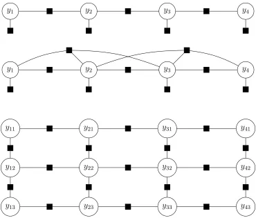
3.2.1 Representing structure with factor graphs

A convenient form of representing the factorization of the scoring function is a factor graph. A factor graph is a bipartite undirected graph G, where there are ` vertices for

the output variablesy1, . . . , y` andF vertices, each representing one factor in the scoring function. Each factor is connected via an edge to each variable in its scope (equivalently, each variable is connected via an edge to each factor it participates in.) Typically, factor graphs are represented visually using round vertices for variables and squares for factors. Factor graphs are useful both as a visual aid to help understand the assumed structure of a model and as a scaffold for efficient inference.

Several examples of common factor graph structures are presented in Figure 3.1.

3.2.2 Complexity of inference

(35)

y1 y2 y3 y4

y11 y21 y31 y41

y12 y22 y32 y42

y13 y23 y33 y43

Figure 3.1: Examples of several common factor graphs. Top: Bigram (1-order) linear-chain model.Middle: Tri-gram (2-order) linear-chain model.Bottom:Grid model.

K values: the messages are defined as follows,

ωc→Yi(k) = max

yc:yi=k

w>fc(x,yc) + X

j∈Yc\i

ωYj→c(yj), (3.2)

ωYi→c(k) = X

c0∈Fi\c

ωc0→Yi(k), (3.3)

where ωc→Yi(k) is the message from factor c to variable i for state k, and ωYi→c is the message from variableito factorcfor statek. If the factor graph is a tree, then the messages

have the following natural intuition. Each variable is separated by its factors from the rest of the variables in the graph; the messageωc→Yi(k)is the maximum score achievable by the rest of the graph (separated fromYibyc) ifYi takes on the valuek. Similarly, the message

(36)

variable Yi if the factor cis not used andYi takes on valuek. Note that certain messages depend upon other messages being precomputed. However, if the factor graph is a tree, then clearly any leaf of the tree can start the process by sending its message to its sole neighbor, and all messages will eventually be computed.

What is the complexity of this inference scheme? For a factor of size d, computing a

single element of the message table involves taking a maximization overd₋1variables, each of which can take on K values. Computing the entire message table is therefore

O(Kd₎_{operations; if there are}_F _{factors, then the entire inference procedure is}_O₍_Kd_F₎_.

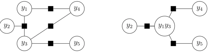
However, if the graph is not a tree (i.e. it contains a cycle), the recursive definition of messages implies that we cannot guarantee exact computation of messages in a finite amount of time. We can still obtain an approximate answer by running message passing scheme anyway; we simply choose an arbitrary start point and re-compute messages as the inputs change, stopping when messages converge or after a pre-determined period of time. This approximate inference scheme is a variant ofloopy belief propagation(LBP), one of many different approximate inference algorithms for cyclic factors. There is a large body of research on approximate inference algorithms that is outside the scope of this thesis; see e.g. Boykov et al. (2001); Koller and Friedman (2009); Murphy et al. (1999); Sontag (2010) for more information.

(37)

y1

y2

y3

y4

y5

y1y3 y2

y4

y5

Figure 3.2: Agglomerating variable states.

3.2.3 Max-margin parameter learning

We now turn to the question of how to learn w to provide useful predictions from the

inference procedure. We follow the structured max-margin framework (Taskar et al., 2005), which aims to solve the following:

min

w,ξ≥0λ||w|| 2₊ 1

n

X

i

ξi s.t. w>f(xi,yi)≥max

y∈Y w >

f(xi,y) + ∆(yi,y) +ξi, ∀i. (3.4) Above,∆is a loss function, such that∆(yi_,_y₎_{measures the difference between the target} outputyi and any given outputy. For most of this work, we use the Hamming loss,

∆(y,y0) = ` X

i=0

1[yi 6=yi0] (3.5)

However, other losses may be used in practice. Intuitively, (3.4) balances a standard`2

reg-ularization term with a penalty for violating a set ofmarginconstraints. In order to satisfy the margin constraints, the true outputyi must have higher score than every alternative y

by margin ∆(yi_,_y₎_{; thus, outputs that are closer to the ground truth (i.e. more correct)} need less margin than those that are farther away, as measured by the loss∆.

(38)

3.3 Trading off computation and expressiveness

As we have seen, the complexity of inference is a function of the structure of the factor graph and of the feature functionsfc(x,y), and inference is often a bottleneck during pa-rameter learning. Therefore, we have a fundamental trade-off between the expressiveness of the model and the computation required to use it effectively.

Linear-chain models. As an example, consider a first-order linear-chain model (Figure

3.1). This model has two types of factors: pairwise factors between consequtive variables

yiandyi+1and unary factors for each variableyi. For ease of notation, we avoid using the

subscriptfcand incorporate the scope of the factor directly, as follows:

f(x,y) = ` X

i=1

f(x, yi, yi+1) +f(x, yi) (3.6)

Since we have ` ₋ 1 pairwise factors and ` unary factors, the complexity of inference

using the message passing algorithm is O(K2_` ₊_K`_{) =} _O₍_K2_`₎_{. We will revisit such}

linear-chain models several times in this thesis; since the features can capture sequential dependencies between predictions, such models are well suited for tasks such as phoneme recognition, handwriting recognition, or visual tracking tasks.

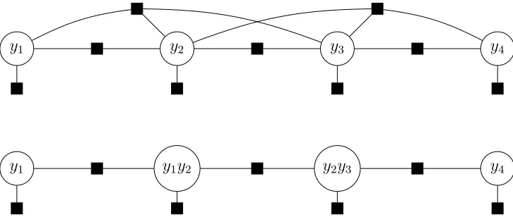
Two channels for more expressiveness. Given the basic first-order linear-chain, we can

introduce more expressiveness into the model through two main channels. The first is simply to incorporate more features into the unary or pairwise terms. For example, when tracking an object in video, optical flow (Horn and Schunck, 1981) – estimating the move-ment of each pixel in an image from one frame to the next – is an expensive but often very useful pairwise feature.

(39)

y1 y2 y3 y4

y1 y1y2 y2y3 y4

Figure 3.3: Removing loops from a trigram model. Top: The trigram linear-chain model contains loops due to incorporating triplets into a new 2-order factor.Bottom:By agglom-erating neighboring states, we obtain a bigram model with no loop, but where the conjoined variables haveK2possible assignments instead ofK.

the tree structure (Figure 3.3). However, we can still perform exact inference by applying the junction method we described in the previous section; we introduce auxiliary variables representing the conjunction of sequential variables as shown in Figure 3.3. Note that the size of the state space of the auxiliary variables increases by a factor of K for each

additional variable we incorporate, so exact inference in ad-gram linear-chain model takes

O(Kd_`₎_{time. Note that we also must introduce consistency requirements into the inference}

procedure: variablesy1y2 andy2y3 must agree on the value of y2 in order to map from an

assignment in the new model back to a sequence of state assignments in the original model. However, these agreement constraints can be easily added by introducing a new indicator feature into the pairwise factors that measures such agreement, taking on the value −∞

when agreement is not satisfied.

3.4 Summary

(40)

explicitly control the the trade-off between expressiveness and computation. As we have seen, there are two primary modes through which we can increase expressiveness: in-creasing factor scope, or adding features to factors. In the next chapters, we propose the SPC/Ensemble-SPC frameworks to address the former and allow for higher order factors or over finer discretizations of the state space, and the DMS/DMS-πframeworks to address

(41)

Chapter 4 Structured Prediction Cascades (SPC)

Overview. As we have discussed, model complexity is limited by computational

con-straints at prediction time in practice, either explicitly by the user or implicitly because of the limits of available computation power. We therefore need to balance expected error with inference time. A common solution is to use heuristic pruning techniques or approx-imate search methods in order to make higher order models feasible. While it is natural and commonplace to prune the state space of structured models, the problem of explicitly learning to control the error/computation tradeoff has not been addressed.

In this chapter, we formulate the problem of learning acascadeof models of increasing complexity that progressively filter a given structured output space, minimizing overall error and computational effort at prediction time according to a desired tradeoff. The key principle of our approach is that each model in the cascade is optimized to accurately filter and refine the structured output state space of the nextmodel, speeding up both learning and inference in the next layer of the cascade. Although complexity of inference increases (perhaps exponentially) from one layer to the next, the state-space sparsity of inference increases exponentially as well, and the entire cascade procedure remains highly efficient. We call our approachStructured Prediction Cascades(SPC).

Contributions. We first introduce SPC in the next section, and propose a novel method

(42)

Algorithm 1:Overview of SPC Inference.

input : Examplex, modelsw0_{, . . . ,}_wT_,_f0_,_fT_.

output: Approximate predictionh(x).

1 initialize_S0 =_Y;

2 fort = 0toT ₋1do

3 Run sparse inference over_Stusing modelwt_,_ft_;

4 Eliminate a subset of low-scoring outputs;

5 OutputSt+1_{for the next model;}

6 Predict using the final level:h(x) = argmax_y_∈ST ψ_wT(x,y)

this filtering method and propose two novel loss functions that bound the accuracy and efficiency of a single level of the cascade. We show how to optimize these losses and pro-vide theoretical analysis in the form of generalization bounds–to our knowledge, these are the first generalization bounds for the accuracy/efficiency trade-off of a structured model. We propose a stage-wise learning algorithm (Algorithm 2) for SPC and apply it to two se-quential prediction tasks: part-of-speech (POS) tagging and handwriting recognition. SPC provides a significant increase in efficiency on the POS tagging task and a dramatic increase in accuracy on the handwriting recognition task.

4.1 Enabling complexity via filtering

Y

(43)

cas-cade for specific problems: for sequential prediction problems, we will define fi _{to be a} linear-chain model of orderi, while for pose estimation problems we will define eachfi_to be a pose model of increasing resolution.

Regardless of the specific layout of the cascade, the goal of each model is to filter out a large subset of the possible values fory without eliminating the correct one. The idea is

that by eliminating possibilities fory, inference in the next model will require searching a

much smaller space. Thus, the filtering process is feed-forward; simpler, faster models are used to quickly eliminate unlikely outputs at first while richer, more complex models can quickly search among the remaining possibilities to produce a final output.

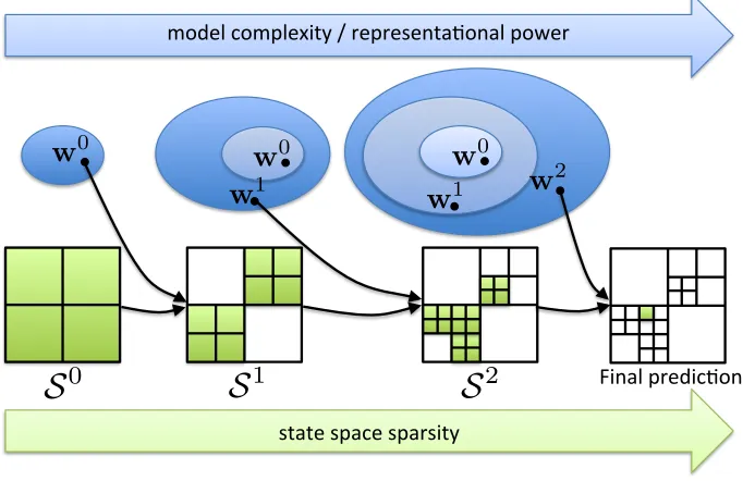
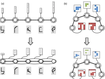
In summary, a high-level overview of the SPC inference framework is given in Algo-rithm 1. Here,St _{denotes a sparse (filtered) version of the output space}_Y_{. The process is} also illustrated in Figure 4.1. See Figure 4.2 for a concrete example of the output of a the first two stages of a cascade for handwriting recognition and human pose estimation. We will discuss how to represent and chooseSt_{in the next section. The key challenge is that}_St are exponential in the number of output variables, which rules out explicit representations. The representation we propose is implicit and concise. It is also tightly integrated with parameter estimation algorithm forwtthat optimizes the overall accuracy and efficiency of

the cascade.

4.2 Cascaded inference with max-marginals

In order to represent and filter low-scoring outputs, we usemax-marginals, for reasons that we detail below. For any value of yc, we define the max-marginal ψw?(x,yc) to be the maximum score of any full outputythat is consistent with the (partial) assignmentyc:

ψ_w?(x,yc), max

y0:y0_c=yc

ψw(x,y0). (4.1)

Max-marginals can be computed exactly and efficiently for any factor cin low-treewidth

graphs, although the computational cost is exponential in |c_| (the number of variables in

(44)

model&complexity&/&representa2onal&power&

state&space&sparsity&

Final&predic2on&

S

2

S

1

S

0

w

0

_w

0

_w

0

w

1

_w

1

w

2

Figure 4.1: A high-level overview of the SPC inference framework. As the cascade pro-gresses, the representational power of the models increases, yet tractability is maintained by sufficient filtering of the state space.

over any subset of variables c, not just the factors used in the feature function f; for

ex-ample, in Section 5.5.2, we compute max-marginals over single variables (i.e., yc = yj) when performing human pose estimation, but at increasingly higher resolutions. On the other hand, in Section 4.5 we compute max-marginals over increasingly large factors for sequence models (e.g. bigram, trigrams, and quadgrams).

Exact computation of max-marginals for a factorcrequires the same amount of time to

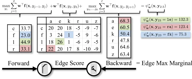
run as standard exact MAP inference. This process is visualized in Figure 4.3: once for-ward and backfor-ward sum messages have been computed for MAP inference, the max-marginal for a given value yc is simply the sum of the scoreψw(x,yc)plus the incoming messages to the variables in c. Note that in practice, both stages of computation become

faster as the output space becomes increasingly sparse as the input proceeds through the cascade. This algorithm can also compute the maximizing assignment for eachyc,

y?_w(x, yc),argmax y0:y0_c=yc

(45)

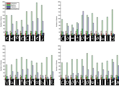
al ec el er ce le re !b ca la le ra bc bl br b h u c f l r a e k r u z c l r a e f g n o p !"#$ !%#$

(46)

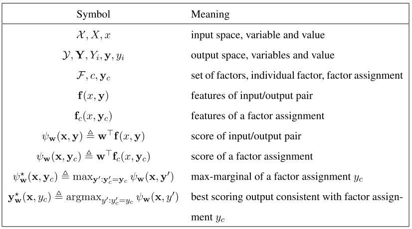
Symbol Meaning

X, X, x input space, variable and value

Y,Y, Yi,y, yi output space, variables and value

F, c,yc set of factors, individual factor, factor assignment

f(x,y) features of input/output pair

fc(x,yc) features of a factor assignment

ψw(x,y),w>f(x,y) score of input/output pair

ψw(x,yc),w>fc(x,yc) score of a factor assignment

ψ?

w(x,yc),maxy0:y0_c=ycψw(x,y

0₎ _{max-marginal of a factor assignment}_y

c

y?

w(x, yc),argmaxy0:yc0=ycψw(x, y

0₎ _{best scoring output consistent with factor}

assign-mentyc

Table 4.1: Summary of key notation.

We call y?

w(x,yc) the argmax-marginal orwitness for yc (it might not be unique, so we break ties in an arbitrary but deterministic way).

Once max-marginals have been computed, we filter the output space by discarding any factor assignmentsycfor whichψw?(x,yc)≤tfor a thresholdt(Figure 4.4). This filtering rule has two desirable properties for the cascade that follow immediately from the definition of max-marginals:

Lemma 1(Safe Filtering). Ifψw(x,y)> t, then∀c ψw?(x,yc)> t.

Lemma 2(Safe Lattices). Ifmaxy0ψw(x,y0)> t, then∃y∀c ψ?w(x,yc)> t.

By Lemma 1, ensuring that the score of the true label ψw(x,y) is greater than the threshold is sufficient (although not necessary) to guarantee that no marginal assignment

ycconsistent with the true global assignmentywill be filtered. This condition will allow us to define a max-marginal based loss function that we propose to optimize in Section 4.3 and will analyze in Section 4.4. Lemma 2 follows from Lemma 1, which states that so long as the threshold is less than the maximizing score, there always exists a global assignmenty

(47)

c 33.7 f 23.0 l 44.9 r 33.1

a 68.3 e 60.5 k 50.4 r 47.8 u 64.6 z 63.4 a e k r u z

c 20 20 18 -5 -9 -7 f 3 24 1 -5 9 -6 l 18 26 1 -6 -9 -5 r 22 20 17 8 -10 -9

= Edge Max Marginal Forward Edge Score Backward

+w>_f₍_x_{, y}

2, y3)+ max y4,...,y`

` X

j=3

w>_f₍_x_{, y}

j, yj+1)

max

y1

2 X

j=1

w>_f₍_x_{, y}

j 1, yj) = ?w(x,y2:3)

?

w(x,y23=le) = 132.3 ?

w(x,y23=ra) = 123.4 ?

w(x,y23=fk) = 75.3

Figure 4.3: Computing max-marginals over bigrams via message passing. The input is the same as in Figure 4.2. Once forward and backward messages have been computed, the max-marginal is simply the sum of incoming messages and the score of the factor over bigrams.

2 guarantees that |Si+1_{| ≥} ₁ _{in the SPC algorithm introduced above, and therefore the}

cascade will always produce a valid output. Note that neither property generally holds for standard sum-product marginals p(yc|x)of a log-linear CRF (where p(y|x) ∝ eψw(x,y)), which motivates our use of max-marginals.

The next component of the inference procedure is choosing a threshold t for a given

inputx(Figure 4.4). Note that the threshold cannot be defined as a single global value but

should instead depend strongly on the input x and ψw(x,·) since scores are on different scales for different x. We also have the constraint that computing a threshold function

(48)

!b !h br bl ul hl hf hc bf hr le la ra ca ck rk ce re fe lk fa fk el ec al kc le ce lo lg !u bc uf ur uc ac

kl co

lp M ax M ar gi na l F il te re d a t Error at F il te re d a t =0 . 5 ↵ =0

= 0.5

⌧w,0(x)

w(x,brace)

⌧w,0.5(x)

max

y w(x,y)

? (w

x

,

yc

)

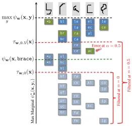
Figure 4.4: Thresholding bigrams using max-marginals. The input is the same as in Fig-ure 4.2. The sparse set of unfiltered bigrams is shown at each position according to the max-marginal score. The bigrams corresponding to the correct label sequence, brace, are highlighted in green. The green dashed line indicates the score of the correct label se-quence. Note that the max-marginals of the correct sequence are at least the score of the correct sequence. The black dashed line indicates the maximum score of any sequence, which is the maximum filtering threshold. The largest max-marginal values are all ex-actly equal to this score. The red dashed lines indicate two candidate filtering thresholds

(49)

the max-marginals:

τw,α(x) =αmax

y ψw(x,y) + (1−α) 1 P

c∈F|Yc| X

c∈F X

yc∈Yc

ψ?_w(x,yc). (4.3)

Choosing a threshold using (4.3) is therefore equivalent to picking aα _∈ [0,1). Note that

τw,α(x)is a convex function ofw(in fact, piece-wise linear), which combined with Lemma 1 will be important for learning the filtering models and analyzing their generalization. In our experiments, we found that the distribution of max-marginals was well centered around the mean, so that choosingα_≈0resulted in_≈50%of max-marginals being eliminated on average. Asαapproaches1, the number of max-marginals eliminated rapidly approaches 100%.1

In summary, the inner loop of the SPC algorithm can be detailed as follows. The sparse output spaceSi_{is a list of valid assignments}_y

cfor each factorcin the modelfi(e.g., Figure 4.2):

Si

=_{Yc | ∀c∈ F} (list of valid factor values for all factors) (4.4)

Next, sparse max-sum message passing is used to compute max-marginalsψ?

w(x,yc)(4.1) for each valueyc ∈ Yc of each factor cof interest. Finally, for a givenα, a threshold is computed and low-scoring values ofψ?

w(x,yc)are eliminated. Depending on the model in the next layer of the cascade, further transformation of the states may be necessary: For example, in the coarse-to-fine pose cascade (Section 6.3.2), valid 2-D locations for each limb are halved either vertically or horizontally to produce finer-resolution states for the next model (Figure 4.2b).

4.3 Learning structured prediction cascades

When learning a cascade, we have two competing objectives that we must trade off:

• Accuracy: Minimize the number of errors incurred by each level of the cascade to

ensure an accurate inference process in subsequent models.

(50)

• Efficiency:Maximize the number of filtered max-marginals at each level in the

cas-cade to ensure an efficient inference process in subsequent models.

Given a training set, we can measure the accuracy and efficiency of our cascade, but what is unknown is the performance of the cascade on test data. In section 4.4, we provide a guarantee that our estimates of accuracy and efficiency will be reasonably close to the true performance measures with high probability. This suggests that optimizing parameters to achieve a desired trade-off on training data is a good idea.

We begin by quantifying accuracy and efficiency in terms of max-marginals, as used by SPC. We define thefiltering lossLf to be a 0-1 loss indicating a mistakenly eliminated correct assignment. As discussed in the previous section, Lemma 1 states that an error can only occur if ψw(x,y) ≤ τw,α(x). We also define the efficiency lossLe to simply be the proportion of unfiltered factor assignments.

Definition 1 (Filtering loss). A filtering error occurs when a max-marginal of a factor

assignment of the correct outputyis pruned. We define filtering loss as

Lf(x,y;w, α) = 1[ψw(x,y)≤τw,α(x)]. (4.5)

Definition 2 (Efficiency loss). The efficiency loss is the proportion of unpruned factor

assignments:

Le(x,y;w, α) = 1 P

c∈F|Yc| X

c∈F,yc∈Yc

1[ψ?_w(x,yc)> τw,α(x)]. (4.6)

We now turn to the problem of learning parameters wand tuning of the threshold

pa-rameterαfrom training data. We have two competing objectives, accuracy (_Lf) and effi-ciency (Le), that we must trade off. Note that we can trivially minimize either of these at the expense of maximizing the other. If we set (w, α) to achieve a minimal threshold such

that no assignments are ever filtered, thenLf = 0andLe = 1. Alternatively, if we choose a threshold to filter every assignment, then Lf = 1 whileLe = 0. To learn a cascade of practical value, we can minimize one loss while constraining the other below a fixed level

(51)

Algorithm 2:Forward Batch Learning of Structured Prediction Cascades.

input : Data{(xi_,_yi₎_}n

1, featuresf0, . . . ,fT and parametersα0, . . . , αT

−1

output: Cascade parametersw0, . . . ,wT

1 initialize_S0(xi_{) =} _Y₍_xi₎_{for each example.;}

2 fort = 0toT ₋1do

3 Optimize (4.8) with sparse inference over the valid set_Stto findwt_;

4 GenerateSt+1(xi)from_St(xi)by filtering low-scoring factor assignmentsyc:

ψ_w?t(xi,yc)≤τwt_,αt(xi)

5 LearnwT to maximize (3.4) over final sparse state spaces_ST(xi);

of minimizing efficiency loss while constraining the filtering loss to be below a desired tolerance.

We express the cascade learning objective for a single level of the cascade as a joint optimization overwandα:

min

w,α EX,Y [Le(X, Y;w, α)] s.t. EX,Y [Lf(X, Y;w, α)]≤. (4.7) We solve this problem for a single level of the cascade as follows. First, we define a con-vex upper-bound (4.8) on the filter errorLf, making the problem of minimizingLf convex inw(givenα). We learnwto minimize filter error for several settings ofα (thus

control-ling filtering efficiency). Given several possible values for w, we optimize the objective

(4.7) over α directly, using estimates of_Lf and Le computed on a held-out development set, and choose the best w. Note that in Section 4.4, we present a theorem bounding the

deviation of our estimates of the efficiency and filtering loss from the expectation of these losses.

For the first step of learning a single level of the cascade, we learn the parameterswfor

a fixedαusing the following convex margin optimization problem:

SP C : min

w

λ

2||w||

2₊ 1 n

X

i

Enabling More Accurate and Efficient Structured Prediction

University of Pennsylvania

ScholarlyCommons

Enabling More Accurate and Efficient Structured

Prediction

David Joseph Weiss

Enabling More Accurate and Efficient Structured Prediction

Acknowledgements

Contents

List of Tables

List of Illustrations

Chapter 1

Introduction

1.1 Thesis Overview

Chapter 2

Related Work

2.1 Controlling computation of multi-class classification

2.1.1 Computational trade-offs during model selection

2.1.2 Predicting with fixed test-time budgets

2.1.3 Resource allocation for batch testing

2.1.4 Classifier cascades

2.1.5 More general multi-stage decision systems

2.1.6 Feature extraction policies

2.2 Related approaches for structured prediction

2.2.1 Coarse-to-fine reasoning

2.2.2 Early stopping cascade

2.2.3 Prioritized inference

2.2.4 Meta-learners/predicting model accuracy

2.2.5 Applications of preliminary works

2.3 Summary

Chapter 3

Structured Prediction: An Overview

3.1 Supervised learning

3.2 Structured prediction

3.2.1 Representing structure with factor graphs

3.2.2 Complexity of inference

3.2.3 Max-margin parameter learning

3.3 Trading off computation and expressiveness

3.4 Summary

Chapter 4

Structured Prediction Cascades (SPC)

4.1 Enabling complexity via filtering

Y

4.2 Cascaded inference with max-marginals

S

S

S

w

w

w

w

w

w

4.3 Learning structured prediction cascades

_w

_w

_w