https://doi.org/10.5194/nhess-18-1535-2018 © Author(s) 2018. This work is distributed under the Creative Commons Attribution 3.0 License.
Estimating grassland curing with remotely sensed data
Wasin Chaivaranont1, Jason P. Evans1, Yi Y. Liu1,2, and Jason J. Sharples3
1ARC Centre of Excellence for Climate Systems Science and Climate Change Research Centre, UNSW, Sydney, NSW 2052, Australia
2School of Geographical Sciences, Nanjing University of Information Science and Technology, Nanjing, 210044, China 3School of Physical, Environmental and Mathematical Sciences, UNSW, Canberra, ACT 2600, Australia
Correspondence:Wasin Chaivaranont ([email protected]) Received: 15 March 2017 – Discussion started: 11 April 2017
Revised: 14 May 2018 – Accepted: 19 May 2018 – Published: 4 June 2018
Abstract.Wildfire can become a catastrophic natural hazard, especially during dry summer seasons in Australia. Severity is influenced by various meteorological, geographical, and fuel characteristics. Modified Mark 4 McArthur’s Grassland Fire Danger Index (GFDI) is a commonly used approach to determine the fire danger level in grassland ecosystems. The degree of curing (DOC, i.e. proportion of dead material) of the grass is one key ingredient in determining the fire dan-ger. It is difficult to collect accurate DOC information in the field, and therefore ground-observed measurements are rather limited. In this study, we explore the possibility of whether adding satellite-observed data responding to veg-etation water content (vegveg-etation optical depth, VOD) will improve DOC prediction when compared with the existing satellite-observed data responding to DOC prediction mod-els based on vegetation greenness (normalised difference vegetation index, NDVI). First, statistically significant rela-tionships are established between selected ground-observed DOC and satellite-observed vegetation datasets (NDVI and VOD) with an r2 up to 0.67. DOC levels estimated us-ing satellite observations were then evaluated usus-ing field measurements with an r2 of 0.44 to 0.55. Results suggest that VOD-based DOC estimation can reasonably reproduce ground-based observations in space and time and is compa-rable to the existing NDVI-based DOC estimation models.
1 Introduction
Wildfire can be responsible for major environmental dam-age or changes to ecosystems (Cobb et al., 2016; Gazzard et al., 2016; Mistry et al., 2016). One of the important com-ponents in determining the severity of wildfire is fuel avail-ability. Wildland fuels can vary considerably, both spatially and temporally (Stambaugh et al., 2011). Various interpre-tations and characterisations of fuel have been made in past studies as a key contribution to assessing wildfire potential (Hudec and Peterson, 2012; Jurdao et al., 2012; Sharples et al., 2009b; Stambaugh et al., 2011; Yebra et al., 2013). Fuel can also be quantified by its age or the time since the last fire (Bradstock et al., 2010). Since this paper uses numbers of abbreviations that may not be familiar to the reader, please refer to the Appendices for the list of acronyms.
2015). In climatological studies, DOC is often assumed to be 100 % (Pitman et al., 2007). This leads to an overestimation of areas experiencing high levels of fire danger and hence provides only a weak indication of where to focus resources of fire agencies. An accurate, spatially and temporally ex-plicit estimate of DOC would provide more useful guidance to these agencies.
Measuring DOC in the field is a tedious and expensive task, especially when an accurate assessment of curing is re-quired. Anderson et al. (2011) suggested that current meth-ods for measuring DOC still present problems. The visual assessment method, which relies on field observers to esti-mate the general curing value based on their expertise and a visual guide, is subjective and can often be unrepresentative of DOC of the entire area. Destructive sampling approaches can provide accurate field-based observation, but is a labour intensive task. Thus, Anderson et al. (2011) offered a simple field-based method utilising a levy rod, based on the modified point quadrant method of pasture assessment; the approach involves counting the number of live and dead touches on a thin steel rod that was driven into the ground. It was sug-gested that this approach can be applied across Australia with higher accuracy than current visual assessment methods (An-derson et al., 2011).
Apart from ground measurement, DOC can be estimated using satellite remotely sensed data, but it is limited by the satellite sensors’ capability, e.g. spatial resolution and var-ious atmospheric interferences. Dilley et al. (2004) estab-lished a relationship between curing and normalised differ-ence vegetation index (NDVI, a proxy of vegetation canopy greenness) by estimating live fuel moisture content from NDVI and relating it to curing via an exponential function using a finite difference Levenberg–Marquardt method (Dil-ley et al., 2004; Rouse et al., 1973). Newnham et al. (2011) showed that estimation of curing using a relative green-ness (RG) approach that was based on NDVI distribution provided more accurate estimation of curing than a direct linear regression between curing and NDVI. Chladil and Nunez (1995) used curing derived from a soil dryness index model and NDVI to predict soil and fuel moisture content. Various optical-based vegetation indices computed from re-mote sensing reflectance products can also be developed into a satellite-based model integrated with ground observations to predict curing (Martin et al., 2015; Turner et al., 2011). These methods, though vastly different in their approaches, achieved good results for their set objectives, but they tend to focus on particular applications. It should also be noted that optical-based remote sensing products, including NDVI, are affected by cloud cover and aerosols. Some studies explicitly acknowledge challenges presented by cloud effects and when there are both forest and water bodies in the same NDVI pixel, which results in an erroneous grassland interpretation (Allan et al., 2003; Chladil and Nunez, 1995). However, if appropriately detailed aerosol data are available, atmospheric correction can mitigate the aerosol effect on NDVI.
Currently, there are satellite-based DOC products over Australia provided by the Bureau of Meteorology. The prod-ucts have 500 m spatial resolution and 8-day temporal reso-lution and are based on two past studies (Martin et al., 2015; Newnham et al., 2010). There are five separate satellite-based DOC models; four are from Newnham et al. (2010) and one is from Martin et al. (2015). All satellite-based DOC mod-els here are based on optical and near-infrared wavelength bands. We would like to investigate whether including a re-cent passive microwave-based satellite product can improve the DOC estimation over Australia.
A passive microwave-based remote sensing vegetation product, referred to as vegetation optical depth (VOD), has been developed recently (Meesters et al., 2005). VOD is primarily sensitive to vegetation water content, including both leafy and woody components (Guglielmetti et al., 2007; Jackson and Schmugge, 1991; Kerr and Njoku, 1990). Un-like the traditional optical-based vegetation indices, such as NDVI, VOD is minimally influenced by the atmospheric conditions due to its longer wavelength and stronger pen-etration capacity (Jones et al., 2009). However, it has a coarser spatial resolution (0.1◦) in comparison with optical-based products, which is a consequence of the low energy microwave emissions from the Earth’s surface. It has been demonstrated that VOD can capture the changes in vege-tation water content over different land cover types at the global scale, including grassland, cropland, savannas, trop-ical forests, and boreal forests (Liu et al., 2013a, b, 2015). A recent study on estimating fire severity based on VOD changes also demonstrated that VOD has high correlation with aboveground biomass in Australian tropical savannahs that includes a large area of northern grassland with anr2 of 0.96 (Chen et al., 2018). Also, NDVI and VOD provide complementary information and can comprehensively char-acterise vegetation dynamics when combined (Andela et al., 2013).
There are two objectives of this study. The first is to ex-plore the possibility of whether adding the VOD (respond-ing to vegetation water content) will improve DOC predic-tion when compared with existing NDVI-based (responding to vegetation greenness) DOC prediction model. The second is to implement the satellite-based DOC estimation (both our and existing models) into GFDI to investigate whether better fire severity predictions can be achieved in grassland envi-ronments.
2 Materials
2.1 Satellite-based products
product used here for computing NDVI is an 8-day prod-uct, which has less noise than the daily prodprod-uct, and its spa-tial resolution is 0.005◦(∼500 m). This product is obtained from the website of the Remote Sensing at National Compu-tational Infrastructure (NCI) MODIS Land Product for Aus-tralia (Paget and King, 2008). It is produced from original tiles provided by the US Geological Survey (USGS) for Aus-tralia with a starting date of 18 February 2000.
The 8-day NDVI data are derived from the MODIS re-flectance dataset using the following:
NDVI=ρ2−ρ1 ρ2+ρ1
, (1)
whereρ1andρ2are spectral reflectance measurements ob-tained from the visible (red) and near-infrared regions, re-spectively. During the conversion, to ensure the quality of data, only pixels with ideal quality in all bands and a view angle zenith of less than 60◦ were kept for the analysis, as suggested by Newnham et al. (2011). The spatial resolution is kept at 0.005◦.
The VOD dataset used here is retrieved from the Ad-vanced Microwave Scanning Radiometer – Earth Observing System (AMSR-E) and derived using the Land Parameter Retrieval Model (LPRM) approach from which soil mois-ture and VOD are retrieved simultaneously (Meesters et al., 2005; Owe et al., 2001). Several assumptions are made in the LPRM approach, including canopy surface temperature equal to soil surface temperature, a constant single scattering albedo, same vegetation parameters for both horizontal and vertical polarisations, and minimal effect of surface rough-ness (Meesters et al., 2005; Owe et al., 2001). Uncertain-ties in soil moisture and VOD retrievals are expected with these assumptions. The evaluation of LPRM soil moisture over Australia showed that the temporal patterns of satellite-based and in situ soil moisture agree very well (Draper et al., 2009; Gevaert et al., 2016). This agreement suggests a rea-sonable separation of temporal patterns of soil moisture and VOD, while uncertainties may exist in the absolute magni-tudes of these two variables.
VOD has a spatial resolution of 0.1◦(∼10 km) and nearly daily temporal resolution (Parinussa et al., 2014). The time period covered by AMSR-E is from 2 June 2002 to 3 Octo-ber 2011, but we used a 9-year range from 4 July 2002 to 26 June 2011 in our analysis by excluding the beginning and the end of the AMSR-E records. The same time period is also used for the MOD09A1 NDVI dataset.
VOD data, which have a near daily temporal resolution, are converted to an 8-day average product to reduce noise and ensure complete coverage over Australia (10 to 45◦S and 110 to 160◦E) per temporal interval. The grid cells with ra-dio frequency interference (RFI) are excluded from our anal-ysis. RFI is caused by man-made transmitters, such as radars and wireless communications. These transmitters can be op-erated in the same frequency range as passive microwave ob-servation, including VOD. Thus, natural signals captured by
passive microwave observations are sometimes contaminated with RFI (de Nijs et al., 2015).
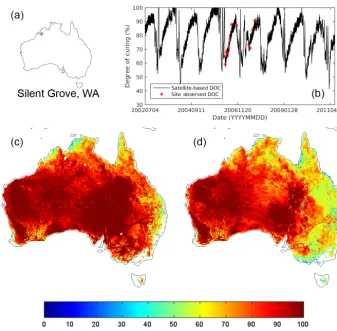
An example comparison time series of VOD and NDVI from July 2002 to June 2011 at one of the observed DOC sites, Silent Grove, WA (17.131◦S, 125.374◦E), can be seen in Fig. 1. It is shown that both VOD and NDVI have a sim-ilar seasonal cycle. Vegetation types that are present within the VOD (0.1◦) and NDVI (0.005◦) pixel influence the differ-ences in VOD and NDVI behaviour. The difference between VOD and NDVI spatial resolution can be clearly seen in the example 2◦by 2◦spatial maps around the Silent Grove area (Fig. 1). We use both VOD and NDVI together to combine their strengths.
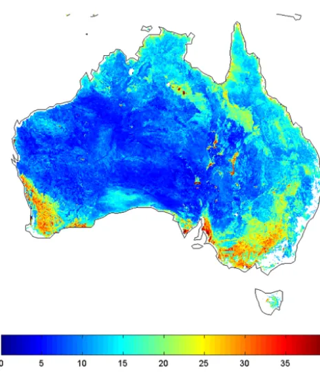
The global 0.05◦ land cover map based on the MODIS MCD12C1 product is used for classifying the dominant land cover type within each VOD pixel. The land cover classifi-cation system is as proposed by the University of Maryland (UMD scheme) (Hansen et al., 2000). Figure 2 shows the 0.05◦land cover type map of Australia, with observed cur-ing sites marked with crosses. The land cover map used here is from year 2010.
A burned area product from MODIS is acquired for fur-ther evaluation of the recalculated GFDI from satellite-based DOC results. The monthly archived MODIS burned area map re-projected for Australia is obtained from Remote Sensing at the NCI site (Paget and King, 2008). There are two sep-arate MODIS burned area products: the MCD45A1 and the MCD64A1. The MCD64A1 burned area product is preferred over MCD45A1, since it was proven to be more accurate (Andela and van der Werf, 2014; Padilla et al., 2015; Ruiz et al., 2014). Its spatial specification is exactly the same as the MODIS reflectance dataset, with temporal availability from August 2000 onwards. To ensure high quality of the burned pixels, only pixels with the valid data flag from the provided quality control file are included in the analysis. Over 99 % of pixels from mid-2002 to mid-2011 are classified as un-burned. To reduce the number of prescribed burns and other low power anomalies detected by the burned area product, a fire radiative power (FRP, unit: MW) from MODIS active fire product (MCD14ML) is used to mask out low severity fires. 2.2 Ground-based curing observations
Figure 1.Example vegetation optical depth (VOD) and normalised difference vegetation index (NDVI) time series(b)and spatial maps
(c)for VOD and(d)for NDVI, at Silent Grove, WA (17.131◦S, 125.374◦E). The star (∗) indicates the location of the time series on a map of Australia(a).
Figure 2.MCD12C1 land cover type map for Australia (Hansen et al., 2000). The locations of 23 valid observed degree of curing (DOC) sites are marked with crosses.
dates (Anderson et al., 2011). Three types of data collection approaches were used: visual estimation, levy rod method, and destructive sampling. Due to the number and availabil-ity of data as well as their accuracy, only observed DOC
To identify robust relationships between the site-observed and remotely sensed DOC, a number of site criteria must be met. Sites meeting these criteria were used for calibration of the VOD and NDVI satellite-based DOC models, while all of the valid records were used for evaluation. One major factor in deciding the site selection is the land cover prop-erties of the observed DOC site. The 0.05◦land cover type map (MCD12C1) is used for classifying the site location land cover (Hansen et al., 2000). Since 0.1◦VOD pixel is covered by 2 by 2 0.05◦ land cover pixels, the corresponding 2 by 2 pixels of land cover type for each observed curing site can be acquired. The land cover type and homogeneity of each observed DOC site can then be determined; the site is con-sidered to have a homogeneous land cover only if all four land cover pixels corresponding to the VOD pixel are the same. In case of a site with heterogeneous land cover type, the dominant land cover with the most pixels out of four will be considered as the representative land cover. All observed DOC sites can be categorised into the following land cover types: evergreen broadleaf forest, open shrubland, savannas, woody savannas, grasslands, croplands, and urban.
According to the land cover information for each 0.1◦ VOD pixel, sites identified as evergreen broadleaf forest pix-els were removed from the analysis. There are three out of 37 sites situated in the evergreen broadleaf forest: Darnum, VIC (mixed grass); Simcocks, WA (improved pasture); and Neerim South, VIC (mixed grass). Even though actual loca-tions of all observed curing sites were in grassy areas, the VOD signal is a mixture of grassland and forest when the sites are surrounded by dense forests within the same 0.1◦ pixel.
All sites were also examined to ensure a negative correla-tion between VOD and the in situ DOC data. That is, since VOD is a proxy for water content in aboveground biomass, an overall negative correlation between VOD and curing is expected. If this is not the case, then there is likely some other activity within the 0.1◦pixel that disrupts this basic relation-ship; this effect was found in three sites: Durran Durra, NSW (native grass); Monaro, ACT (improved pasture); and Parry Lagoons, WA (native grass). The sites without the negative correlation with VOD also had no correlation with NDVI, suggesting other land cover types were dominating the sig-nal. Thus, 6 out of 37 sites are excluded from the analysis.
In addition, there are eight sites (Umbigong, ACT – native grass; Kilcunda, VIC – improved pasture; Tooradin, VIC – improved pasture; Tooradin North, VIC – improved pasture; Caldermeade Park, VIC – improved pasture; Kaduna Park, VIC – improved pasture; Hobart Airport, TAS – native grass; and Jerona, QLD – native grass) in which VOD data are not available. Most of these are due to sites being located near the coast or a large body of water, where the VOD signal is strongly influenced by the water itself. With the remaining 23 out of 37 sites, several site selection criteria were applied for the calibration phase. The criterion used here to main-tain consistency in observation time series requires sites to
have at least eight consecutive records – records are consid-ered consecutive when they are separated by no more than 15 days. Only the consecutive series of records within the selected sites are included in the analysis for the calibration phase. This ensures that the derived model contains the tem-poral evolution of DOC within years. Only 5 out of 23 sites are retained for this group, containing a total of 122 (out of 238 total) observations. The selected sites are Majura, ACT (improved pasture); Tidbinbilla, ACT (mixed grass); Ballan, VIC (improved pasture); Murrayville 1, VIC (native grass); and Murrayville 2, VIC (improved pasture). Multiple linear regression models of VOD and NDVI were then calibrated with the observed curing from the final selected sites. 2.3 Meteorological datasets
To further assess the usability of the satellite-based curing acquired from the VOD and NDVI model, the GFDI is puted. Additional meteorological data needed for GFDI com-putation are dry bulb or maximum temperature, 15:00 rel-ative humidity, maximum wind speed, and fuel load (Pur-ton, 1982). Since fuel load is often set as a constant value of 0.45 kg m−2 (Sharples et al., 2009a), there are three re-maining input datasets needed. These gridded meteorologi-cal datasets are usually derived from the network of ground observation stations across Australia. The range for these datasets is from 4 July 2002 to 26 June 2011 to exactly match with the VOD 9-year range. Both temperature and relative humidity datasets are acquired from the Australian Water Availability Project (AWAP) (Jones et al., 2009). Note that relative humidity is derived from vapour pressure and temperature data. These AWAP datasets have a 0.05◦ spa-tial and daily temporal resolution with a coverage region of 10 to 44.5◦S and 112 to 156◦E. For maximum wind speed data, the reanalysis maximum daily wind speed is computed from the ERA-Interim wind components dataset, acquired from the European Centre for Medium-Range Weather Fore-casts (ECMWF) (Dee et al., 2011). The reanalysis wind com-ponents dataset is available globally at approximately 0.8◦ spatial resolution at a 6 h interval.
3 Methods
3.1 Developing VOD–NDVI-based dynamic DOC estimates
One of the two alternatives Newnham et al. (2011) proposed is the range-based RG, which can be computed by the fol-lowing Eq. (2):
RG= NDVI−NDVImin
NDVImax−NDVImin
, (2)
where the NDVIminand NDVImaxare the minimum and max-imum NDVI value over a specified time range. Note that we did not attempt to compare the other proposed alternative, the spread-based RG, but only range-based (per pixel) RG. In Newnham et al. (2011), while range-based RG performance is not as good as preferred spread-based RG (r2=0.62 and RMSE=14.2 %), it is still better than plain NDVI (NDVI had r2=0.50 and RMSE=16.4 %, while 2.5-year range-based RG has r2=0.57 and RMSE=15.1 %). Note that while we cannot exactly reproduce the 10-year time range that Newnham et al. (2011) used, since our study time frame is 9 years, we tried various 2.5-year time ranges that over-lapped with the Newnham et al. (2011) study period. How-ever, given the same observed DOC data and NDVI dataset, we were unable to reproduce a result where the RG corre-lation with DOC is stronger than NDVI. Further analysis showed that the RG results were very sensitive to the se-lected time range for the computation, such that results were inconsistent with relatively small differences in the selected range. Due to this, RG is not used in this study and NDVI is used directly in forming a multiple linear regression model to estimate satellite-based curing. Some experimentation re-vealed that the VOD anomalies, computed from the differ-ence between VOD and average VOD over a specified tem-poral range, yield the best correlation with DOC, but only if the VOD anomalies are computed from the range match-ing the in situ DOC observation range for each specific site. The range selection for computing VOD anomalies can be quite problematic, since it can heavily influence the correla-tion result, and no pattern could be found for determining an appropriate VOD range for any other locations outside the observed DOC sites. Thus, we focus our analysis on using the absolute VOD value. The linear regression equation for curing and VOD correlation can be expressed as
C=x1+x2(VOD), (3)
wherex1andx2are the intercept and slope of the relation-ship.
Utilising both VOD and NDVI datasets, the following multiple linear regression equation for estimating DOC can be expanded from Eq. (3) as
C=x1+x2(VOD)+x3(NDVI)+x4(VOD)(NDVI), (4) where x1 tox4 are the intercept and coefficients of VOD, NDVI, and the product of VOD and NDVI (interaction term), respectively. Using a stepwise regression, the calibrated final model with corresponding coefficients can be determined.
The stepwise fit algorithm used here selects the significant terms with the lowestpvalue, which is smaller than the en-trance tolerance, to be included in the model first. Next, the algorithm chooses the next most significant term that is still less than the entrance tolerance. This process is repeated un-til either there are no remaining significant terms or all terms are included in the final model (Draper and Smith, 1998). Af-ter the final model is calibrated, we evaluate the DOC model with all valid (23) observed DOC sites.
3.2 Comparing with existing DOC estimates
We acquire existing satellite-based DOC products available from the Australian Bureau of Meteorology and compare their performance with our model. There are five models available, four based on Newnham et al. (2010) and one based on Martin et al. (2015). We decided to test only one of Newnham’s models – the one with the best overall RMSE (Method B) –and Martin’s model (MapVic). Both Method B and MapVic DOC models are described in Eqs. (5) and (6), as shown below:
CMethod B=237.31−190.14(NDVI)−142.66 ρ
7 ρ6
, (5) CMapVic=113.80−88.41(NDVI)−67.71(GVMI), (6) whereρ6andρ7are spectral reflectance band six and seven from MODIS reflectance dataset and GVMI is the Global Vegetation Monitoring Index (Martin et al., 2015; Newnham et al., 2010). GVMI can be calculated by
GVMI=(ρ2+0.1)−(ρ6+0.02) (ρ2+0.1)+(ρ6+0.02)
, (7)
whereρ2 andρ6 are spectral reflectance band two and six from MODIS reflectance dataset (Ceccato et al., 2002).
To compare both Method B and MapVic model perfor-mance with our model, we evaluate them using the same ob-served DOC sites and evaluation methods. We also computed recalculated GFDI with both Method B and MapVic DOC and assessed their burned area prediction capability.
3.3 Comparing GFDI dynamics using different DOC estimates
Figure 3. Scatter plot of observed degree of curing (DOC) from five calibration sites against VOD, NDVI, and combined VOD and NDVI terms.
GFDI=Q1.027f (C)exp(−1.523+0.0276Tmax −0.2205pH3 pm+0.6422
p Vmax
, (8)
whereQis the fuel load (kg m−2),Tmaxis the dry bulb or daily maximum temperature (◦C), H3 pm is the daily rela-tive humidity at 15:00 (%),Vmaxis the daily maximum wind speed (km h−1), and f (C)is the curing factor. The curing factor can be calculated by
f (C)=exp−0.009432(100−C)1.536, (9) whereCis the grassland DOC (%).
The GFDI is computed on the basis of meteorological in-put data and either a constant DOC at 100 % or satellite-based dynamic curing values. These different GFDI datasets along with the burned area data (MCD64A1) can be used to examine the changes due to variable DOC spatially and temporally. By pairing up burned and unburned pixels with their associated GFDI pixel, we can assess the number of burned and unburned pixels for each GFDI severity level. Using histogram and receiver operating characteristic (ROC) analysis, the difference between original GFDI with constant DOC at 100 % and recalculated GFDI with satellite-based dynamic DOC can be assessed (DeLong et al., 1988; Zweig and Campbell, 1993).
4 Results
4.1 Comparing VOD–NDVI-based and existing DOC estimates
Across all selected observed DOC sites (excluding the for-est areas) from July 2002 to June 2011, ther2of VOD and
Figure 4.Scatter plot of residual observed degree of curing (DOC) from five calibration sites that are unexplained by NDVI against VOD and combined VOD and NDVI terms.
NDVI is 0.52 with an RMSE of 0.11. Using the linear model, as described by Eq. (3), the DOC and VOD correlation result has a significant relationship and anr2of 0.20 with RMSE of 20.80 %. The scatter plot showing the correlation between VOD, NDVI, and combined VOD and NDVI terms is as shown in Fig. 3, while Fig. 4 shows the residual DOC un-explained by NDVI (differences between observed DOC and NDVI-based DOC) against VOD and combined VOD and NDVI terms.
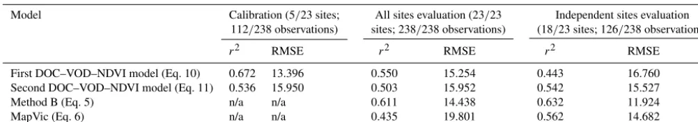
Table 1. Calibration and evaluation of satellite-based degree of curing (DOC) models derived from vegetation optical depth (VOD) and normalised difference vegetation index (NDVI). Evaluating existing estimated DOC models, Method B (Newnham et al., 2010) and MapVic (Martin et al., 2015), are also listed below.
Model Calibration (5/23 sites; All sites evaluation (23/23 Independent sites evaluation 112/238 observations) sites; 238/238 observations) (18/23 sites; 126/238 observations)
r2 RMSE r2 RMSE r2 RMSE
First DOC–VOD–NDVI model (Eq. 10) 0.672 13.396 0.550 15.254 0.443 16.760
Second DOC–VOD–NDVI model (Eq. 11) 0.536 15.950 0.503 15.952 0.542 15.527
Method B (Eq. 5) n/a n/a 0.611 14.438 0.632 11.924
MapVic (Eq. 6) n/a n/a 0.435 19.801 0.562 14.682
C1=145.57−260.82(NDVI)+137.19(VOD)(NDVI) (10) C2=48.70+147.60(VOD)−259.95(VOD)(NDVI) (11) The DOC models are then evaluated with all (23) valid ob-served DOC sites and independent (18) obob-served DOC sites (excludes 5 sites that were used in calibration). The evalu-ation results for the first model are also shown in Table 1, where the evaluated r2 is 0.55 and 0.44 with RMSE of 15.25 and 16.76 % for the evaluation of all sites and indepen-dent sites, respectively. The second model evaluations results haver2of 0.50 and 0.54, with RMSE of 15.95 and 15.53 % for the evaluation of all sites and independent sites, respec-tively. While the evaluations resulted in degradation in model performance over the calibration in most cases, the indepen-dent evaluation of the second model has a slightly better eval-uation performance.
These results can be compared to those obtained using ex-isting remotely sensed DOC estimates which are also shown in Table 1. The MapVic DOC has a lower r2 and higher RMSE, while the Method B DOC has a higherr2and lower RMSE when compared with both of our models in the eval-uation of all sites. This indicates that Method B has the best evaluation among the three models, while MapVic is the worst, and our models sit in the middle between the two. However, during an evaluation of the independent sites, both models with VOD have the worst performance (lowest r2 and RMSE). This result is not entirely surprising as all the observations used here were also used in the calibration of Method B (Newnham et al., 2010), a subset is used in the calibration of our method, and MapVic was developed using an independent visual estimates dataset. That is, there are no independent data available for testing Method B, while both our method and MapVic are being tested against indepen-dent data. While our first and second models do not have ob-vious advantages over one another, since the second model only performs better than the first in the evaluation of the independent sites, we decided to pick the first model as our representative model for further comparison with the exist-ing models from this point, since the terms in the first model were selected based on stepwise fit regression with none of our interference (we intentionally removed the NDVI term
in the second model before applying the stepwise fit regres-sion).
Using the relationship between VOD, NDVI, and observed DOC from the first model, as stated in Eq. (10), we calculated satellite-based DOC for Australia. Figure 5 presents maps of satellite-based DOC data averaged over the summer periods (December, January, February, DJF) for the years 2002–2003 and 2010–2011. From mid-2002 to mid-2011, the overall av-erage curing for the Australian summer period is the highest during 2003 and the lowest during 2011. Note that the pix-els that are classified as any forest types are masked out in white. Comparison time series between satellite-based and site-observed DOC at Silent Grove, WA (same location as shown in VOD and NDVI example comparison in Fig. 1), is also shown at the top of Fig. 4 as an example.
To determine the amount of spatial variation in DOC across Australia, we computed the standard deviation of all valid DOC estimates across the continent within a single time step. All areas that are indicated as forests by the land cover type map are excluded from the analysis. The spatial vari-ation time series can then be plotted for the available time period of mid-2002 to mid-2011, as shown in Fig. 6. Note that the continental mean spatial DOC standard deviation is 20.39 %. This indicates that there is significant spatial vari-ability in DOC that persists across all years, and contains a small seasonal component. For a normally distributed vari-able, 95 % of values would lie within 2 standard deviations, which is±40.78 % in this case. Further analysis of DOC spa-tial standard deviation is as shown in Table 2. This includes seasonal, monthly, and land cover type spatial standard devi-ation of DOC. From both seasonal and monthly spatial stan-dard deviation of DOC, it is shown that DOC has the highest spatial variation during winter, which is especially true for northern Australia (Anderson et al., 2011).
Figure 5. Example satellite-based and site-observed degree of curing (DOC) time series comparison at Silent Grove, WA (17.131◦S, 125.374◦E)(b), where the star (∗) indicate the location of the time series on a map of Australia(a). Satellite-based DOC across Australia during summer (December, January, February) for 2002–2003(c)and 2010–2011(d)are shown with forest areas masked out.
Figure 6. Spatial standard deviation of estimated degree of cur-ing (DOC) time series from 4 July 2002 to 26 June 2011.
Figs. 6 and 7 show the variability in DOC that will impact calculations of fire danger indices.
4.2 Comparing GFDI dynamics using different DOC estimates
Figure 7.Temporal standard deviation of estimated degree of cur-ing (DOC) map from 4 July 2002 to 26 June 2011.
during low to moderate GFDI conditions; in addition, some fires shown in Fig. 9 occur in forested areas where GFDI is not applicable. Nevertheless, they provide a picture of the in-terannual spatial variability in both GFDI and burned area.
The time series plots of recalculated GFDI at Weston Creek, ACT, and Toodyay, WA, for the 2003 and 2010 fire events are shown in Fig. 10. The black line represents the re-calculated GFDI from variable DOC, while the dashed, light green line is for original GFDI with constant DOC at 100 %. These locations are marked with red plus signs on the spatial maps (Fig. 8). Note that the original GFDI time series peaks every year, whereas the recalculated GFDI with variable cur-ing time series shows sudden peaks in the days near major fires. The Weston Creek fire was part of the 2003 Canberra bushfire complex, where multiple fires merged and rapidly propagated from 18 to 22 January 2003, burning 1600 km2 (McLeod, 2003). The weather conditions on 18 January 2003 were extreme with temperature as high as 40◦C and wind exceeding 60 km h−1. The Toodyay fire was much smaller in magnitude, burning just over 30 km2on 29 December 2009. The Weston Creek area is mostly comprised of forest with mixed land cover, whereas the Toodyay area is mostly a mix between croplands and savannas.
Using a burned area observation dataset from MODIS (MCD64A1), we test the effectiveness of GFDI with variable curing in increasing the probability that fires will occur in high GFDI severity levels compared to the probability that fires will occur in low–moderate GFDI
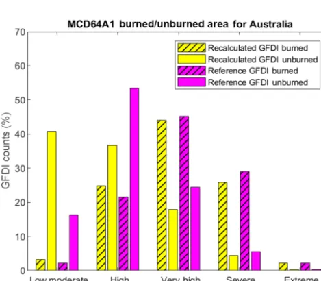
severity levels. Low-intensity fires, such as prescribed burns, are removed from the burned area observation by using the FRP provided in MODIS active fire product (MCD14ML) to mask out burned area that have low FRP. We assume any burned area with FRP lower than 100 MW to be unburned (associated with low–moderate GFDI risk). At each burned and unburned daily data point, the corresponding daily GFDI was calculated. The GFDI histogram in Fig. 11 shows the frequency of satellite-based recalculated GFDIs and constant-based (DOC=100 %) reference GFDIs over burned and unburned areas. Figure 11 shows that the recalculated GFDI places the largest percentage of unburned pixels in the low–moderate GFDI severity class, with∼75 % of all unburned pixels occurring in the low–moderate or high severity classes. Meanwhile the reference (DOC=100 %) GFDI places ∼80 % of unburned pixels in the high, very high, severe, and extreme classes.
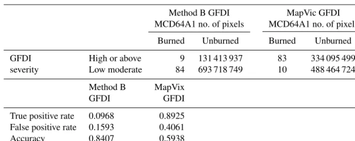
We can evaluate the performance in correctly assigning burned and unburned area for both recalculated and reference GFDI by using the concept of ROC, as described earlier. As-sume that the MCD64A1 burned area map represents the true condition and that the GFDI severity level represents the pre-dicted condition, where the prediction is positive when GFDI level is classified as high or above for a burned area and low– moderate for an unburned area. Table 3 shows the contin-gency table, including both type I (unburned area with high or above GFDI level; false positive) and type II (burned area with low–moderate GFDI level) errors. Though recalculated GFDI has a lower true positive rate of correctly assigning burned area than reference GFDI (0.86 vs. 0.95), it is much better at assigning unburned area correctly, i.e. lower false positive rate (0.38 vs. 0.53). Overall accuracy for recalcu-lated GFDI is higher than the reference GFDI (0.62 vs. 0.47). Both Method B and MapVic DOC are then used to com-pute recalculated GFDI and compare with burned area obser-vation dataset in the same manner as our DOC model. From the ROC analysis in Table 4 for Method B and MapVic recal-culated GFDI, we found that even though Method B has the best DOC evaluation results (highestr2, lowest RMSE) and highest overall recalculated GFDI burned and unburned de-tection accuracy at 0.84, it is the worst at detecting burned area correctly with a true positive rate of only 0.10. This concurs with the findings in Newnham et al. (2010) who found Method B to consistently underpredict DOC, and hence it produces fewer cases of high or above GFDI sever-ity. Our model is in the middle ground between Method B and MapVic in terms of overall accuracy.
5 Discussion
5.1 Evaluation of satellite-based DOC
Table 2. Spatial standard deviation of estimated degree of curing (DOC) by season, month, and land cover type from 4 July 2002 to 26 June 2011.
DOC spatial standard deviation
Season Spatial Month Spatial Land cover type Spatial
SD SD SD
(%) (%) (%)
Autumn (MAM) 20.636 January 19.050 Closed shrublands 11.484 Winter (JJA) 22.895 February 21.354 Open shrublands 13.982 Spring (SON) 18.861 March 21.167 Woody savannas 17.912 Summer (DJF) 19.161 April 20.228 Savannas 13.432 May 20.498 Grasslands 19.105 June 21.770 Croplands 20.995 July 23.231
August 23.634 September 21.971 October 18.305 November 16.325 December 17.276
Figure 9.MCD64A1 burned area map (Ruiz et al., 2014) during summer (December, January, February) 2002–2003(a)and 2009–2010(b)
with forest areas masked out.
Table 3.Referenced and recalculated Grassland Fire Danger Index (GFDI) severity and burned–unburned area contingency table for satellite-based degree of curing (DOC) derived from vegetation optical depth (VOD) and normalised difference vegetation index (NDVI). Reference GFDI is computed from constant DOC at 100 %, while recalculated GFDI is computed from satellite-based DOC.
Recalculated GFDI Reference GFDI (first model) MCD64A1 no. of pixels MCD64A1 no. of pixels
Burned Unburned Burned Unburned GFDI High or above 88 446 894 217 80 319 386 462 severity Low moderate 5 395 703 734 13 523 211 489
Reference Recalculated
GFDI GFDI
(first model) True positive rate 0.9462 0.8602 False positive rate 0.5304 0.3790 Accuracy 0.4696 0.6210
Figure 11. Grassland Fire Danger Index (GFDI) severity level histograms at burned and unburned areas over Australia during 4 July 2002 to 26 June 2011 where the dark and light blue shaded bars are recalculated GFDI with satellite estimated variable degree of curing (DOC), while the green and yellow shaded with diagonal hatch bars are reference GFDI with constant DOC at 100 %.
Newnham et al. (2011) various forms of NDVI were used, in-cluding a straight NDVI linear regression and relative NDVI, as shown in Eq. (2). Their results suggested that a linear re-gression model based on NDVI alone reproduced site obser-vations with an r2of 0.50. The results presented here indi-cate that inclusion of VOD in the regression model yields a comparable performance withr2of 0.44 to 0.55 (with eval-uation of the independent sites being the worst and evalua-tion of all sites being the best performance). However, when we compare the evaluation results with the currently
avail-able satellite-based DOC from the Bureau of Meteorology, the best performer is Method B in bothr2 and RMSE for both evaluation methods (Newnham et al., 2010). We note that this is not a fair comparison as all the data used to eval-uate the models were used to calibrate Method B, regardless of our evaluation methods. MapVic (Martin et al., 2015), in contrast, was developed using a totally independent visual assessment dataset and hence is being evaluated against an independent dataset, regardless of our evaluation methods. Our first model performs better in an evaluation of all sites (include subset of the data for calibration) than the indepen-dent sites, as expected. However, our second model performs better in the evaluation of independent sites than of all sites. Regardless, the overall performance is still not obviously bet-ter than neither Method B or MapVic models. While adding VOD to the DOC estimation model may introduce a compa-rable alternative to the existing optical-based models, there is still no clear advantage of including VOD over the current methods.
An earlier study for estimating DOC directly with NDVI yielded even smaller RMSE of up to 6.3 %, but that partic-ular study is focused on data from only three different sites, within a limited study area of 1 km2 (Dilley et al., 2004). Older studies that have used NDVI data derived from the Na-tional Oceanic and Atmospheric Administration’s (NOAA) Advanced Very High Resolution Radiometer (AVHRR) have the same problem of interference from clouds and atmo-spheric effects, but do not have the advantage that VOD is not affected by clouds or aerosol interference.
5.2 GFDI with various DOC estimates
Table 4.Recalculated Grassland Fire Danger Index (GFDI) severity and burned–unburned area contingency table for degree of curing (DOC) computed with Method B (Newnham et al., 2010) and MapVic (Martin et al., 2015) model. Reference GFDI is computed from constant DOC at 100 %, while recalculated GFDI is computed from satellite-based DOC.
Method B GFDI MapVic GFDI MCD64A1 no. of pixels MCD64A1 no. of pixels
Burned Unburned Burned Unburned GFDI High or above 9 131 413 937 83 334 095 499 severity Low moderate 84 693 718 749 10 488 464 724
Method B MapVix GFDI GFDI True positive rate 0.0968 0.8925 False positive rate 0.1593 0.4061 Accuracy 0.8407 0.5938
0.48 for GFDI with 100 % constant DOC), we found that it is the worst at detecting burned area correctly (true pos-itive rate from best to worst is 0.88 for GFDI with 100 % constant DOC, 0.74 for MapVic, 0.69 for our DOC model, and 0.09 for Method B). Our VOD- and NDVI-based DOC model (first model) has a good balance in having the second best evaluation result and overall recalculated GFDI accuracy with a decent correct burned area detection rate. We note that GFDI is only an indicator for the level of fire risk and does not guarantee that a fire will occur, even at an extreme danger level. However, the improvement in accuracy indicates that inclusion of time- and space-varying DOC estimates makes it much more likely that areas identified at a GFDI severity level of high or above will burn than a low–moderate severity level area.
5.3 Limitations
It is worth noting here that in an operational setting atmo-spheric interference by clouds or smoke will cause gaps in the optical (NDVI) data, though the VOD data remain unaf-fected. We also note that while the VOD data used here were derived from the AMSR-E sensor, which is no longer oper-ational, VOD data derived from currently operating passive microwave sensors, such as the Advance Microwave Scan-ning Radiometer 2 (AMSR2), could be used in an operational setting. It should also be noted that VOD’s moderately coarse resolution of 0.1◦may not be fine enough for use in many ap-plications.
Reducing the chance of incorrectly assigning unburned and burned areas correctly from the ROC analysis made here is purely based on using the burned area map as a true base-line. However, the burned area map may include fires that are deliberately lit in low–moderate conditions, such as pre-scribed burns and fires that the GFDI is not designed for, such as a fire that burns in forested regions. Prescribed burns and low-intensity fires are, however, minimised by applying low FRP threshold, using information from the MODIS
ac-tive fire product. The ROC analysis result here is only used to reinforce the idea that using the reference GFDI with con-stant curing (100 %) leads to overestimating GFDI in some situations and might result in misleading fire danger warn-ings.
The satellite-based DOC produced here is also at a mod-erate spatial resolution, which is a limitation of many satel-lite products. However, DOC in reality can vary over spa-tial scales much finer than the satellite footprint (less than 500 m). As such, our model should only be used as a guide for dynamic, near daily assessment of grassland cur-ing at coarse to moderate spatial scales. This is also true for other satellite-based DOC models, including Method B and MapVic models.
6 Conclusions
Data availability. The following datasets and their associated sources or contact points are as listed below:
– MODIS MOD09A1, MCD16C1, MCD14ML, and MCD64A1 for NDVI computation, land cover type map, active fire prod-uct, and burned area map for Australia are freely available from NASA via Remote Sensing at NCI (mosaicing and regridding by CSIRO): http://remote-sensing.nci.org.au/u39/public/html/ modis/lpdaac-mosaics-cmar/ (Paget and King, 2008).
– AMSR-E VOD dataset for Australia is available upon request by contacting Yi Liu: [email protected].
– Method B and MapVic DOC products information can be found at http://data.auscover.org.au/xwiki/bin/view/Product+ pages/Grassland+Curing+MODIS+BoM (Grant, 2015) and the datasets are downloaded from the following catalogue: http://opendap.bom.gov.au:8080/thredds/catalog/curing_ modis500m8-day/aust/netcdf/catalog.html.
– Observed DOC dataset via visual assessment, levy rod, and destructive methods is available upon request from the follow-ing Bushfire and Natural Hazards Cooperative Research Cen-tre legacy project: http://www.bushfirecrc.com/projects/a14/ grassland-curing (Anderson et al., 2011).
– Maximum daily observed gridded temperature and vapour pressure dataset for Australia are freely available from AWAP: http://www.bom.gov.au/jsp/awap/ (Raupach et al., 2012).
Appendix A: List of variables C degree of curing (%)
C1 estimated degree of curing using our first model, shown in Eq. (10) (%) C2 estimated degree of curing using our second model, shown in Eq. (11) (%) CMethod B estimated degree of curing using Method B model (%) (Newnham et al., 2011) CMapVic estimated degree of curing using MapVic model (%) (Martin et al., 2015) GVMI Global Vegetation Monitoring Index (unitless)
f (C) curing factor (unitless)
H3 pm daily relative humidity at 15:00 (%)
NDVImax maximum NDVI value over a specific time range used for calculating relative greenness (unitless) NDVImin minimum NDVI value over a specific time range used for calculating relative greenness (unitless) Q fuel load (kg m−2)
RG relative greenness (unitless)
Tmax dry bulb or daily maximum temperature (◦C) Vmax daily maximum wind speed (km h−1) x1 coefficient in the linear regression equation x2 coefficient in the linear regression equation x3 coefficient in the linear regression equation x4 coefficient in the linear regression equation
Appendix B: List of acronyms
AMSR-E (Advanced Microwave Scanning one of the sensors aboard Aqua satellite; a passive microwave radiometer; Radiometer – Earth Observing System) stop rotating on 4 October 2011
AMSR2 (Advance Microwave Scanning one of the sensors aboard JAXA’s GCOM-W1 satellite; a passive microwave Radiometer 2) radiometer; currently operating
AVHRR (Advanced Very High Resolution a radiation detection that is used for determining cloud cover and surface
Radiometer) temperature
AWAP (Australian Water Availability Project) a state and trend of the terrestrial water balance monitoring project in Australia
CSIRO (Commonwealth Scientific and independent Australian Federal Government’s scientific research agency Industrial Research Organisation)
DOC (degree of curing) a percentage measurement of dead material in grassland fuel complex ECMWF (European Centre for Medium- independent, intergovernmental organisation producing global numerical Range Weather Forecasts) weather forecasts
ERA-Interim a global reanalysis climate dataset from 1979 to present
LPRM (Land Parameter Retrieval Model) a radiative transfer model for solving surface soil moisture and vegetation optical depth from microwave observation
Modified Mark 4 McArthur’s Grassland fire danger index for grassland ecosystem developed and used in Australia Fire Danger Index (GFDI)
MCD12C1 2010 MODIS land cover type product (University of Maryland scheme)
MCD14ML MODIS fire radiative power product
MCD45A1 daily MODIS burned area product
MCD64A1 daily MODIS burned area product
MOD09A1 8-day MODIS reflectance product on board Terra satellite
MODIS (Moderate Resolution Imaging key instrument abroad Terra and Aqua satellites acquiring data in
Spectroradiometer) 36 spectral bands
NDVI (normalised difference vegetation optical-based satellite product used as proxy for vegetation greenness index)
NCI (National Computational Australia’s highly integrated and high performance research computing
Infrastructure) environment
NOAA (National Oceanic and Atmospheric US government agency working on daily weather forecasts and climate
Administration) monitoring
P value the significance of the results in a statistics hypothesis test where strong evidence against the null hypothesis is indicates by lowpvalue r2(Rsquared) a statistical measurement of the correlation between two variables
RFI (radio frequency interference) interference in microwave-based satellite product (VOD in this case) due to wireless transmission, causing erroneous values in the affected grid pixels RMSE (root mean square error) differences between the values estimated by a model and the observed
values
USGS (US Geological Survey) the US government’s scientific agency studying the landscape, natural resources, and natural hazards of the US
Author contributions. WC, JE, and YL were involved in initial re-search planning and experiments design. For the rest of the study, including the analysis of the results, paper writing, and manuscript proofreading, all authors (WC, JE, YL, and JS) were involved.
Competing interests. The authors declare that they have no conflict
of interest.
Acknowledgements. We would like to acknowledge the following
parties:
– NASA for making MODIS data freely available;
– NCI and CSIRO for making a freely available preprocessed MODIS data for Australia;
– Bureau of Meteorology for making freely available satellite-based DOC dataset and continue to generate and distribute the data products set up by the AWAP project;
– Bushfire and Natural Hazards Cooperative Research Centre and its partner agencies for allowing us to use their observed DOC dataset from their legacy project;
– AWAP for making daily Australia climate gridded dataset freely available;
– ECMWF for making ERA-Interim reanalysis gridded dataset freely available.
Edited by: J. G. Pinto
Reviewed by: Célia Gouveia and one anonymous referee
References
Allan, G., Johnson, A., Cridland, S., and Fitzgerald, N.: Application of NDVI for predicting fuel curing at landscape scales in northern Australia: can remotely sensed data help schedule fire manage-ment operations?, Int. J. Wildland Fire, 12, 299–308, 2003. Andela, N. and van der Werf, G. R.: Recent trends in
African fires driven by cropland expansion and El Nino to La Nina transition, Nat. Clim. Change, 4, 791–795, https://doi.org/10.1038/nclimate2313, 2014.
Andela, N., Liu, Y. Y., van Dijk, A. I. J. M., de Jeu, R. A. M., and McVicar, T. R.: Global changes in dryland vegeta-tion dynamics (1988–2008) assessed by satellite remote sensing: comparing a new passive microwave vegetation density record with reflective greenness data, Biogeosciences, 10, 6657–6676, https://doi.org/10.5194/bg-10-6657-2013, 2013.
Anderson, S. A. J., Anderson, W. R., Hollis, J. J., and Botha, E. J.: A simple method for field-based grassland curing assessment, Int. J. Wildland Fire, 20, 804–814, https://doi.org/10.1071/WF10069, 2011.
Berrisford, P., Dee, D. P., Poli, P., Brugge, R., Fielding, M., Fuentes, M., Kållberg, P. W., Kobayashi, S., Up-pala, S., and Simmons, A.: The ERA-Interim archive Ver-sion 2.0, ECMWF, https://www.ecmwf.int/en/forecasts/datasets/ archive-datasets/reanalysis-datasets/era-interim, 2011.
Bradstock, R. A., Hammill, K. A., Collins, L., and Price, O.: Effects of weather, fuel and terrain on fire severity in topographically
diverse landscapes of south-eastern Australia, Landsc. Ecol., 25, 607–619, https://doi.org/10.1007/s10980-009-9443-8, 2010. Ceccato, P., Gobron, N., Flasse, S., Pinty, B., and Tarantola, S.:
Designing a spectral index to estimate vegetation water content from remote sensing data: Part 1: Theoretical approach, Remote Sens. Environ., 82, 188–197, https://doi.org/10.1016/S0034-4257(02)00037-8, 2002.
Chen, X., Liu, Y. Y., Evans, J. P., Parinussa, R. M., van Dijk, A. I. J. M., and Yebra, M.: Estimating fire severity and car-bon emissions over Australian tropical savannahs based on pas-sive microwave satellite observations, Int. J. Remote Sens., https://doi.org/10.1080/01431161.2018.1460507, in press, 2018. Chladil, M. and Nunez, M.: Assessing grassland moisture and biomass in Tasmania – the application of remote-sensing and empirical-models for a cloudy environment, Int. J. Wildland Fire, 5, 165–171, 1995.
Cobb, R. C., Meentemeyer, R. K., and Rizzo, D. M.: Wild-fire and forest disease interaction lead to greater loss of soil nutrients and carbon, Oecologia, 182, 265–276, https://doi.org/10.1007/s00442-016-3649-7, 2016.
Cruz, M. G., Gould, J. S., Kidnie, S., Bessell, R., Nichols, D., and Slijepcevic, A.: Effects of curing on grassfires: II. effect of grass senescence on the rate of fire spread, Int. J. Wildland Fire, 24, 838–848, https://doi.org/10.1071/WF14146, 2015.
Dee, D. P., Uppala, S. M., Simmons, A. J., Berrisford, P., Poli, P., Kobayashi, S., Andrae, U., Balmaseda, M. A., Balsamo, G., Bauer, P., Bechtold, P., Beljaars, A. C. M., van de Berg, L., Bid-lot, J., Bormann, N., Delsol, C., Dragani, R., Fuentes, M., Geer, A. J., Haimberger, L., Healy, S. B., Hersbach, H., Hólm, E. V., Isaksen, L., Kållberg, P., Köhler, M., Matricardi, M., McNally, A. P., Monge-Sanz, B. M., Morcrette, J.-J., Park, B.-K., Peubey, C., de Rosnay, P., Tavolato, C., Thépaut, J.-N., and Vitart, F.: The ERA-Interim reanalysis: configuration and performance of the data assimilation system, Q. J. Roy. Meteorol. Soc., 137, 553– 597, https://doi.org/10.1002/qj.828, 2011.
DeLong, E. R., DeLong, D. M., and Clarke-Pearson, D. L.: Com-paring the areas under two or more correlated receiver operating characteristic curves: a nonparametric approach, Biometrics, 44, 837–845, 1988.
de Nijs, A. H. A., Parinussa, R. M., de Jeu, R. A. M., Schellekens, J., and Holmes, T. R. H.: A methodology to determine radio-frequency interference in AMSR2 observations, IEEE T. Geosci. Remote, 53, 5148–5159, https://doi.org/10.1109/TGRS.2015.2417653, 2015.
Dilley, A. C., Millie, S., O’Brien, D. M., and Edwards, M.: The relation between Normalized Difference Vegetation Index and vegetation moisture content at three grassland locations in Victoria, Australia, Int. J. Remote Sens., 25, 3913–3930, https://doi.org/10.1080/01431160410001698889, 2004. Draper, C. S., Walker, J. P., Steinle, P. J., de Jeu, R. A. M.,
and Holmes, T. R. H.: An evaluation of AMSR-E derived soil moisture over Australia, Remote Sens. Environ., 113, 703–710, https://doi.org/10.1016/j.rse.2008.11.011, 2009.
Draper, N. R. and Smith, H.: Applied regression analysis, 3rd Edn., Wiley-Interscience, Hoboken, NJ., 1998.
Gevaert, A. I., Parinussa, R. M., Renzullo, L. J., van Dijk, A. I. J. M., and de Jeu, R. A. M.: Spatio-temporal evaluation of resolution enhancement for passive microwave soil moisture and vegetation optical depth, Int. J. Appl. Earth Obs. Geoinform., 45, 235–244, https://doi.org/10.1016/j.jag.2015.08.006, 2016.
Gill, A. M., King, K. J., and Moore, A. D.: Australian grassland fire danger using inputs from the GRAZPLAN grassland simulation model, Int. J. Wildland Fire, 19, 338–345, 2010.
Grant, I.: Grassland Curing – MODIS, Bushfire CRC algo-rithms, Australia and states coverage, Bureau of Meteorol-ogy, http://data.auscover.org.au/xwiki/bin/view/Product+pages/ Grassland+Curing+MODIS+BoM, 2015.
Guglielmetti, M., Schwank, M., Mätzler, C., Oberdörster, C., Vanderborght, J., and Flühler, H.: Measured mi-crowave radiative transfer properties of a deciduous forest canopy, Remote Sens. Environ., 109, 523–532, https://doi.org/10.1016/j.rse.2007.02.003, 2007.
Hansen, M. C., Defires, R. S., Townshend, J. R. G., and Sohlberg, R.: Global land cover classification at 1km resolution using a de-cision tree classifier, Int. J. Remote Sens., 21, 1331–1365, 2000. Hudec, J. L. and Peterson, D. L.: Fuel variability follow-ing wildfire in forests with mixed severity fire regimes, Cascade Range, USA, Forest Ecol. Manage., 277, 11–24, https://doi.org/10.1016/j.foreco.2012.04.008, 2012.
Jackson, T. J. and Schmugge, T. J.: Vegetation effects on the mi-crowave emission of soils, Remote Sens. Environ., 36, 203–212, 1991.
Jones, D. A., Wang, W., and Fawcett, R.: High-quality spatial cli-mate data-sets for Australia, Aust. Meteorol. Oceanogr. J., 58, 233–248, 2009.
Jurdao, S., Chuvieco, E., and Arevalillo, J. M.: Mod-elling fire ignition probability from satellite estimates of live fuel moisture content, Fire Ecol., 7, 77–97, https://doi.org/10.4996/fireecology.0801077, 2012.
Kerr, Y. H. and Njoku, E. G.: A semiempirical model for in-terpreting microwave emission from semiarid land surfaces as seen from space, IEEE T. Geosci. Remote, 28, 384–393, https://doi.org/10.1109/36.54364, 1990.
Kidnie, S., Cruz, M. G., Gould, J., Nichols, D., Anderson, W., and Bessell, R.: Effects of curing on grassfires: I. fuel dynamics in a senescing grassland, Int. J. Wildland Fire, 24, 828–837, 2015. Liu, Y. Y., Evans, J. P., McCabe, M. F., de Jeu, R. A. M., van Dijk,
A. I. J. M., Dolman, A. J., and Saizen, I.: Changing climate and overgrazing are decimating Mongolian steppes, PLoS ONE, 8, e57599, https://doi.org/10.1371/journal.pone.0057599, 2013a. Liu, Y. Y., van Dijk, A. I. J. M., McCabe, M. F., Evans, J. P., and
de Jeu, R. A. M.: Global vegetation biomass change (1988–2008) and attribution to environmental and human drivers, Global Ecol. Biogeogr., 22, 692–705, https://doi.org/10.1111/geb.12024, 2013b.
Liu, Y. Y., van Dijk, A. I. J. M., de Jeu, R. A. M., Canadell, J. G., McCabe, M. F., Evans, J. P., and Wang, G.: Recent reversal in loss of global terrestrial biomass, Nat. Clim. Change, 5, 470– 474, https://doi.org/10.1038/nclimate2581, 2015.
Martin, D., Chen, T., Nichols, D., Bessell, R., Kidnie, S., and Alexander, J.: Integrating ground and satellite-based observa-tions to determine the degree of grassland curing, Int. J. Wildland Fire, 24, 329–339, 2015.
McLeod, R.: Inquiry into the operational response to the Jan-uary 2003 bushfires in the ACT, ACT Government, Can-berra, Australia, available at: http://pandora.nla.gov.au/pan/ 35870/20030923-0000/www.cmd.act.gov.au/mcleod_inquiry/ Documents/Final/McLeodInquiry.pdf (last access: 1 June 2018), 2003.
Meesters, A. G. C. A., de Jeu, R. A. M., and Owe, M.: Analytical derivation of the vegetation optical depth from the microwave polarization difference index, IEEE Geosci. Remote Sens. Lett., 2, 121–123, https://doi.org/10.1109/LGRS.2005.843983, 2005. Mistry, J., Bilbao, B. A., and Berardi, A.: Community owned
so-lutions for fire management in tropical ecosystems: case studies from Indigenous communities of South America, Philos. T. Roy. Soc. B, 371, 20150174, https://doi.org/10.1098/rstb.2015.0174, 2016.
Newnham, G. J., Grant, I., Martin, D., and Anderson, S. A. J.: Improved methods for assessment and prediction of grassland curing, Bushfire Cooperative Research Centre, Melbourne, VIC, 2010.
Newnham, G. J., Verbesselt, J., Grant, I. F., and Anderson, S. A. J.: Relative Greenness Index for assessing curing of grassland fuel, Remote Sens. Environ., 115, 1456–1463, https://doi.org/10.1016/j.rse.2011.02.005, 2011.
Noble, I. R., Gill, A. M., and Bary, G. A. V.: McArthur’s fire-danger meters expressed as equations, Aust. J. Ecol., 5, 201–203, https://doi.org/10.1111/j.1442-9993.1980.tb01243.x, 1980. Owe, M., De Jeu, R., and Walker, J.: A methodology for surface
soil moisture and vegetation optical depth retrieval using the mi-crowave polarization difference index, IEEE T. Geosci. Remote, 39, 1643–1654, https://doi.org/10.1109/36.942542, 2001. Padilla, M., Stehman, S. V., Ramo, R., Corti, D., Hantson, S.,
Oliva, P., Alonso-Canas, I., Bradley, A. V., Tansey, K., Mota, B., Pereira, J. M., and Chuvieco, E.: Comparing the accuracies of re-mote sensing global burned area products using stratified random sampling and estimation, Remote Sens. Environ., 160, 114–121, https://doi.org/10.1016/j.rse.2015.01.005, 2015.
Paget, M. J. and King, E. A.: MODIS Land data sets for the Australian region, Internal Report, CSIRO Marine and Atmo-spheric Research Black Mountain, Canberra, Australia, avail-able at: http://remote-sensing.nci.org.au/u39/public/html/modis/ lpdaac-mosaics-cmar/ (last access: 1 June 2018), 2008. Parinussa, R. M., Yilmaz, M. T., Anderson, M. C., Hain,
C. R., and de Jeu, R. A. M.: An intercomparison of re-motely sensed soil moisture products at various spatial scales over the Iberian Peninsula, Hydrol. Process., 28, 4865–4876, https://doi.org/10.1002/hyp.9975, 2014.
Peterson, S. H., Roberts, D. A., and Dennison, P. E.: Map-ping live fuel moisture with MODIS data: a multiple re-gression approach, Remote Sens. Environ., 112, 4272–4284, https://doi.org/10.1016/j.rse.2008.07.012, 2008.
Pitman, A. J., Narisma, G. T., and McAneney, J.: The impact of cli-mate change on the risk of forest and grassland fires in Australia, Climatic Change, 84, 383–401, https://doi.org/10.1007/s10584-007-9243-6, 2007.
Purton, C. M.: Equations for the McArthur mark 4 grassland fire danger meters, Meteorol. Note, 147, 1–12, 1982.
Rouse, J. W., Haas, R. H., Schell, J. A., and Deering, D. W.: Mon-itoring vegetation systems in the Great Plains with ERTS, Third ERTS Symp., 10–14 December 1973, Washington, D.C., USA, 309–317, 1973.
Ruiz, J. A. M., Lázaro, J. R. G., del Cano, I. Á., and Leal, P. H.: Burned area mapping in the North American boreal forest us-ing Terra-MODIS LTDR (2001–2011): A comparison with the MCD45A1, MCD64A1 and BA GEOLAND-2 products, Remote Sens., 6, 815–840, https://doi.org/10.3390/rs6010815, 2014. Sharples, J. J., McRae, R. H. D., Weber, R. O., and
Gill, A. M.: A simple index for assessing fire dan-ger rating, Environ. Model. Softw., 24, 764–774, https://doi.org/10.1016/j.envsoft.2008.11.004, 2009a.
Sharples, J. J., McRae, R. H. D., Weber, R. O., and Gill, A. M.: A simple index for assessing fuel mois-ture content, Environ. Model. Softw., 24, 637–646, https://doi.org/10.1016/j.envsoft.2008.10.012, 2009b.
Stambaugh, M. C., Dey, D. C., Guyette, R. P., He, H. S., and Marschall, J. M.: Spatial patterning of fuels and fire hazard across a central U.S. deciduous forest region, Landsc. Ecol., 26, 923– 935, https://doi.org/10.1007/s10980-011-9618-y, 2011. Turner, D., Lewis, M., and Ostendorf, B.: Spatial indicators of fire
risk in the arid and semi-arid zone of Australia, Ecol. Indic., 11, 149–167, https://doi.org/10.1016/j.ecolind.2009.09.001, 2011. Vermote, E. F. and Vermeulen, A.: Atmospheric correction
algo-rithm: spectral reflectance (MOD09), University of Maryland, Maryland, USA, 1999.
Yebra, M., Dennison, P. E., Chuvieco, E., Riano, D., Zylstra, P., Hunt Jr., E. R., Danson, F. M., Qi, Y., and Jurdao, S.: A global review of remote sensing of live fuel moisture content fofire dan-ger assessment: Moving towards operational products, Remote Sens. Environ., 136, 455–468, 2013.