www.the-cryosphere.net/9/663/2015/ doi:10.5194/tc-9-663-2015
© Author(s) 2015. CC Attribution 3.0 License.
On producing sea ice deformation data sets from
SAR-derived sea ice motion
S. Bouillon1,2and P. Rampal1,2
1Nansen Environmental and Remote Sensing Center, Bergen, Norway 2Bjerknes Centre for Climate Research, Bergen, Norway
Correspondence to: S. Bouillon ([email protected])
Received: 10 September 2014 – Published in The Cryosphere Discuss.: 10 October 2014 Revised: 11 March 2015 – Accepted: 12 March 2015 – Published: 9 April 2015
Abstract. We propose a method to reduce the error generated when computing sea ice deformation fields from synthetic aperture radar (SAR)-derived sea ice motion. The method is based on two steps. The first step consists of using a trian-gulation of the positions taken from the sea ice trajectories to define a mesh on which a first estimate of sea ice defor-mation is computed. The second step consists of applying a specific smoother to the deformation field to reduce the ar-tificial noise that arises along discontinuities in the sea ice motion field. This method is here applied to RADARSAT Geophysical Processor System (RGPS) sea ice trajectories having a temporal and spatial resolution of about 3 days and 10 km, respectively. From the comparison between unfiltered and filtered fields, we estimate that the artificial noise causes an overestimation of about 60 % of opening and closing. The artificial noise also has a strong impact on the statistical dis-tribution of the deformation and on the scaling exponents es-timated with multifractal analysis. We also show that a simi-lar noise is present in the deformation fields provided in the widely used four-point deformation RGPS data set. These findings may have serious implications for previous studies as the constant overestimation of the opening and closing could lead to a large overestimation of freezing in leads, salt rejection and sea ice ridging.
1 Introduction
Sea ice motion can be retrieved from satellite synthetic aper-ture radar (SAR) images using cross-correlation techniques and feature tracking algorithms (Kwok et al., 1990; Fily et al., 1990; Hollands and Dierking, 2011). Sea ice
deforma-tion is then estimated by computing the spatial derivatives of the sea ice motion. The most popular data set providing both sea ice motion and deformation is the RADARSAT Geophys-ical Processor System (RGPS) data set (Kwok, 1998). It cov-ers the western Arctic for the period 1996–2008 at tempo-ral and spatial resolution of about 3 days and 10 km, respec-tively.
As deformation determines sea ice opening (i.e., positive divergence) and closing (i.e., negative divergence), it may be used to estimate important global quantities, such as the ice production in leads, with some assumptions on sea ice growth and redistribution (Kwok et al., 1995). Using the RGPS data set, Kwok (2006) estimated that deformation-related ice production is about 25–40 % of the winter ice pro-duction in both the perennial and seasonal ice zones. Kwok et al. (2008) also showed that the deformation-related ice production derived from the RGPS data set is up to 2 times higher than the one estimated by numerical models, imply-ing a potential underestimate of the associated sea ice–ocean feedbacks.
(2009, 2011) showed that classical sea ice models do not cap-ture these statistical properties.
The estimation of these global quantities (e.g., total open-ing/closing) and statistical properties (e.g., spatial scaling ex-ponents) may be impacted by errors in sea ice deformation data. Uncertainty on deformation is usually seen as a con-sequence of motion tracking errors that depend on the algo-rithm and parameters used. Lindsay and Stern (2003) esti-mated the standard deviation of the error in area change to be about 1.4 km2for a 10 by 10 km cell when the tracking error (i.e., tie point) is about 100 m. This error estimate is equiv-alent to the level of significance of 0.005 per day for 3-day intervals estimated by Kwok and Cunningham (2002), and used to determine the error on ice production as being less than 1 % of the total.
However, two other sources of error can be identified. Both are linked to the definition of the boundary of the cell (usu-ally quadrangle) over which deformation is computed. Lind-say and Stern (2003) showed that unrealistic deformation is often obtained when this boundary is too irregular. Also, spu-rious openings and closings (that we will refer to as artificial noise hereafter) are caused by unfavorable orientation of the cell boundary relative to the discontinuities in the sea ice mo-tion field, also called dynamic discontinuities, slip lines or linear kinematic features (LKFs). Lindsay and Stern (2003) evaluated the standard deviation of the error in area change due to the boundary definition to be about 3.2 km2 for a 10 by 10 km square cell, which is more than twice the error from tracking mentioned above. Kwok (2006) stated that this arti-ficial noise would lead to an overestimation of the ice volume production, although no precise number was given. Lindsay et al. (2003) proposed to reduce this error by combining cells together, but this solution reduces the benefits of having high-resolution data and reduces the spatial range over which one could perform scaling analysis. The error in estimating defor-mation has also been studied by Thorndike (1978) for large spatial scales (from 100 to 500 km), but such an analysis is only valid for homogeneous and isotropic fields and does not apply to small-scale deformation as explained in Lind-say et al. (2003).
This paper proposes a method to avoid unrealistic values and to significantly reduce the noise obtained when com-puting sea ice deformation from SAR-derived motion and presents an example of its application to sea ice trajecto-ries coming from the RGPS data set. The complete method is described in Sect. 2. In Sect. 3, we discuss the quality of the obtained deformation fields and analyze the impacts of removing the artificial noise on the estimated global open-ing/closing and on the spatial scaling of the deformation. Section 4 concludes the paper with a discussion on poten-tial improvements of the method and on implications of our findings for the existing literature.
Figure 1. Example of the divergence (a, c, e) and shear (b, d, f)
obtained for the single-crack test case at a normalized resolution of 0.1. The relative displacement parallel and normal to the crack (black line) are set to 0.01 and 0, respectively. (a) and (b) corre-spond to the unfiltered deformation fields, (c) and (d) to the de-formation fields filtered with a classical smoothing kernel and (e) and (f) to the deformation fields filtered with our smoother. Tri-angles in white show the kernel defined for the triangle in green. With both smoothers the kernel corresponds to cells that can be reached by crossing a maximum ofnedges (heren=7). The classi-cal smoother takes all the cells into account, whereas our smoother only takes into account the cells whose deformation is above a given threshold.
2 Method
The method we developed is based on two steps. The first step consists of defining a mesh by doing a triangulation of a set of tracked points. For each individual triangular cell, the deformation is calculated using the motion of its three nodes estimated from the tracking procedure. The second step con-sists of applying a specific smoother to the obtained defor-mation fields to reduce the artificial noise.
2.1 Application to simple test cases
In order to present the method, we first define a simple setup on a square domain having a normalized area equal to 1. In this domain, tracked points are distributed uniformly with a mean distancedbetween them (see for example Fig. 1 with d=0.1).dis hereafter called the normalized resolution.
In the first test case, a single crack is defined (black line in Fig. 1). This crack passes by the center of the domain and makes an angleθwith the horizontalxaxis. We want to sim-ulate a discontinuous displacement field that is induced by the presence of that crack. To do so, we keep the points lo-cated below the crack (lower part of the domain in Fig. 1) fixed, and we require the points above the crack (upper part of the domain in Fig. 1) to move with the same displace-ment. The two components of the imposed displacement,up andun, correspond to the displacement parallel and normal to the crack, respectively.
displace-ment are obtained by calculating the following contour inte-grals as in Kwok et al. (2008) around the boundary of each triangle:
ux=
1 A
I
udy, (1)
uy= −
1 A
I
udx, (2)
vx=
1 A
I
vdy, (3)
vy= −
1 A
I
vdx, (4)
whereAis the cell area. For example,uxis approximated by
ux=
1 A
m X
i=1 1
2(ui+1+ui)(yi+1−yi), (5) wherem=3 and subscriptm+1=1. The shearshearand divergencedivdeformations are computed as
shear=
q
ux−vy2+ uy+vx2, (6)
div=ux+vy. (7)
In the case of a slip line,unis set to 0. No opening or closing should occur and shear should have the same value along the crack. Figure 1a and b show the divergence and shear com-puted for such a case, withup=0.01 andun=0. The diver-gence field exhibits spurious positive (opening) and negative (closing) values along the slip line. The shear field also ex-hibits some noise, but that is hardly visible in the figure.
This artificial noise generates an overestimation of the to-tal opening (and closing). In our test cases, the opening (and closing) error is defined as the absolute difference between the total opening (and closing) computed from the geometry of the problem and the total opening (and closing) computed from the integration of the positive (and negative) divergence given by the method. Repeating the slip line experiment 100 times, with θ varying from −arctan(0.2) to +arctan(0.2) and with different meshes, we find that the root mean square (rms) error per unit crack is about 20 % of the sliding dis-tanceupfor both the opening and closing. In other words, with a 100 km long crack and a sliding distance of 1 km, the artificial opening (and closing) would be about 20 km2. It is particularly interesting to note that this error does not depend on the normalized resolutiond(we tested withdequal to 0.1, 0.01 and 0.001).
When repeating the same test case with quadrangles in-stead of triangles, we found a rms error of about 18 % of the sliding distanceup. For comparison, Lindsay and Stern (2003) found an error per unit crack of about 15 % of the sliding distance, for a similar test case on a mesh made of square cells. This analysis shows that using triangles gen-erates an increase of only about 10 % of the opening (and closing) error compared to using quadrangles. This increase
of the error is minor compared to the advantages of using tri-angles. Triangulation methods are more flexible. It roughly doubles the number of deformation estimates and increases the resolution at which deformation is defined. For the rest of this paper, we thus only present results on triangular meshes, but the method could also be applied to other type of meshes. In order to remove the artificial noise in the deformation fields, one could apply an isotropic smoother over all the cells of the mesh. We here denoteCthe list of all the cells, and for each cellc∈Cwe define the kernelKc⊂Cas the subset of
cells that can be reached by crossing a maximum ofnedges. An example of kernel withn=7 is shown in Fig. 1c and d. The size of the kernel is noted|Kc|. For the example shown
in Fig. 1c and d,|Kc|is equal to 87. The components of the
filtered deformation are then defined as an area-weighted av-erage over the cells of the kernel. For example, the filtered value foruxon the cellcis defined as
eu c x=
P k∈KcA
kuk x P
k∈KcA
k . (8)
This method reduces part of the artificial noise but is not ap-propriate since it ruins the localization of the shear and adds unreal deformation to non-deforming cells. It also modifies the spatial scale at which the deformation is defined, result-ing in a modification of the value of the shear along the crack. With the single-crack case, the area-weighted average of the shear for the cells cut by the crack is found to be inversely proportional ton.
We propose a better method based on the fact that the de-formation is by nature constant along a linear kinematic fea-ture. Averaging motion derivatives along these features could then filter out the noise without spoiling the information on the real deformation. Contrary to the isotropic smoother pre-sented here above, the mean value of the shear obtained with the second method in the single-crack case does not vary as a function ofn. In other words, the scale at which the defor-mation is defined remains constant with the second method, which can be seen as an anisotropic smoother. In the case of a regular mesh and a single crack aligned with thexaxis, we verified that the area-weighted average of the shear along the crack is strictly constant whatever the value ofn. For the rest of this study, we consider that our method does not modify the spatial scale at which the deformation is defined. In some cases this assumption may not be verified, for example, when two cracks intersect or when the treated cells do not belong to a linear kinematic feature. Two metrics will be used to an-alyze the error caused by intersecting cracks and to evaluate the proportion of treated cells that can actually be considered as cracks.
To detect the cells that are involved in the mapping of each linear kinematic feature, we define a threshold for total defor-mation (
q
fil-0 5 10 15 20 25 0
0.05 0.1 0.15 0.2 0.25 0.3 0.35 0.4 0.45
Normalized ridging/opening error
n
u n=0 u n=u /8 p u n=u /4 p
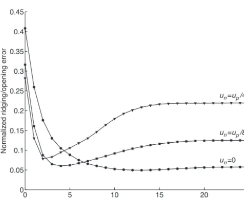
Figure 2. Root mean square closing/opening error normalized by
upand computed from 100 realizations of the single-crack (disks)
and double-crack test cases (squares and triangles) at the resolution 0.1. For all curves,up=0.01.
tering is applied on the cells where deformation is below the threshold. We denoteS the list of all the selected cells. For each cells∈S, we define the kernelKs⊂Sas the subset of cells that can be reached by crossing only selected contigu-ous cells and a maximum ofnedges.|Ks|is the size of the kernel. In the case of the single crack the size of the kernel is alway equal to 2n+1, except for the kernels whose center is close to the boundary of the domain. The kernel size may then be as low asn+1. Our method preserves the localiza-tion of the deformalocaliza-tion by avoiding mixing the deformalocaliza-tion between LKFs (i.e., cells where the deformation is intense) and the surrounding rigid plates (i.e., cells where deforma-tion is almost 0). Moreover, the way the smoothing kernels are built using contiguous cells ensures that deformation be-tween LKFs that are not connected will not be averaged to-gether.
The proposed method relies on two parameters: the defor-mation threshold that determines which cells are selected and parameter nthat determines how far we extend the kernel. In our test cases, the threshold value is chosen to be small enough to select all the deforming cells. For application to real data, the choice of this parameter is critical and is de-tailed in Sect. 2.2. The impact of parameter n on the total error, defined as the sum of the opening and closing errors, is shown in Fig. 2 (line with disk symbols). This error, when normalized by the sliding distanceup, decreases from about 40 % to a residual error that depends on the normalized reso-lution. For a resolution of 0.1, the residual error (i.e., the error remaining forn > d−1) is about 5 % as shown in Fig. 2. Sim-ple analytical developments (not shown here) and numerical experiments withd ranging [0.1–0.001] show that the resid-ual error for the single-slip case is proportional to the
nor-0
-0.04 0.04
0
-0.04 0.04
Figure 3. Example of the unfiltered (left panel) and filtered (right
panel) divergence obtained for the double-crack test case at a nor-malized resolution of 0.1. The domain is divided into three blocks. Points below the principal crack are fixed. Points above the princi-pal crack experience the same displacementun, perpendicular to the
principal crack (hereun= −0.0025) but have distinct tangent
com-ponents:up for the block on the left (hereup=0.01) andu0pfor
the block on the right of the secondary crack (hereu0p=0.0125). Triangles in white show the kernel defined for the triangle in green. In this example, the parameternis equal to 3.
malized resolution, whereas the initial error does not depend on the normalized resolution.
The two other curves in Fig. 2 (with square and triangle symbols) correspond to the normalized errors found for ex-periments considering a secondary crack as shown in Fig. 3. The domain is now divided into three blocks. Points below the principal crack are still fixed. Points above the principal crack experience the same displacementun, perpendicular to the principal crack, but have distinct tangent componentsup for the block on the left oru0pfor the block on the right of the secondary crack.
To get one crack opening while the other is closing,u0p is defined as up−un. The example in Fig. 3 is given for up=0.01 andun= −0.0025, so the principal crack should be closing whereas the secondary crack should be opening. Before filtering, the computed divergence field is highly pol-luted by the noise. Once the deformation is filtered (here withn=3), the divergence field better matches the expected opening and closing. At the intersection of the two cracks, however, the solution may be incorrect, as the method does not distinguish cracks when they intersect and thus aver-ages deformation over cells belonging to different cracks. It should be also noted that at the intersections of two cracks the size of the kernel|Ks|may be as high as 3n+1 (for three-branch intersections as in Fig. 3) or 4n+1 (for four-branch intersections).
This mixing of intersecting cracks explains why the nor-malized error (triangle and square symbols in Fig. 2), after having rapidly decreased for smallnas in the single-crack case, starts to increase for larger n. This simple test case shows that the shape of this function depends on the ratio
un
up and that the optimal value forn would be 4 for un up =
1 8 and 2 for un
up = 1
−12 −10 −8 −6 −4
x 105
−4 −3 −2 −1 0 1 2 3
x 105
x [km]
y [km]
Divergence rate
[/day]
−0.04 −0.03 −0.02 −0.01 0 0.01 0.02 0.03 0.04
Figure 4. Unfiltered divergence rate computed from the RGPS sea
ice trajectory data set and corresponding to the pair of images taken attk−1=3 February 2007 at 17:44:00 UTC andtk=7 Febru-ary 2007 at 17:26:35 UTC.
presented here. In real cases, to define an optimal value forn is more difficult as it would depend on the number of inter-secting cracks and on the local ratio between divergence and shear. For this study, we chose to use a constant parameter n, and its reference value is fixed atn=3. To validate the choice of the method’s parameters (i.e.,nand the deforma-tion threshold), we present in Sect. 3 another metric based on a multifractal scaling analysis of the deformation fields. 2.2 Application to RGPS sea ice trajectories
The RGPS Lagrangian displacement product provides trajec-tories of sea ice “points” initially located on a 10 km regu-lar grid (http://rkwok.jpl.nasa.gov/radarsat/lagrangian.html). The positions of these points are updated when two succes-sive images are available and treated by the tracking algo-rithm. The time interval between two updates is typically 3 days. Spatial coordinates are given in the SSM/I polar stere-ographic projection, with the origin of the Cartesian grid lo-cated at the North Pole and the negativeyaxis aligned to the 45◦W meridian.
The RGPS Lagrangian deformation product provides the deformation of each cell (which is quadrangle) of the origi-nal grid. The deformation of a cell is updated each time the position of all its nodes are updated. This method has a seri-ous problem because cells may become so distorted that spa-tial derivatives are ill-defined. As the RGPS deformation data set does not provide for each cell the position of its node, it is not possible to filter the data to avoid this problem. This prob-lem is specific to the RGPS deformation product and would not appear if each pair of images was treated separately with its own grid as in the GlobICE Image Pair product (http:
//www.globice.info) and in the ENVISAT Geophysical Pro-cessor System (EGPS) (http://rkwok.jpl.nasa.gov/envisat/).
To tackle these problems, we reprocessed the RGPS La-grangian displacement product to build a new deformation data set called the RGPS Image Pair Product. We first iden-tify the tracked points corresponding to each pair of images (i.e., the set of points whose position has been updated at the exact same date and with the same time interval). We gener-ate a Delaunay triangulation of these points. Then we com-pute the deformation over what we consider as being well-shaped cells, i.e., only for triangles having an area between 5 and 400 km2, their angles higher than 5◦or all their edges shorter than 25 km. We also only keep meshes if they have at least 200 nodes, and we discard single and pairs of trian-gles that are not connected to other cells. Figure 4 shows an example of a mesh and a sea ice divergence field after the processing of the data corresponding to one pair of images. Artificial noise, characterized by a succession of highly neg-ative and positive values, is clearly visible and, as expected, is mainly located along lines.
Using triangles instead of quadrangles roughly doubles the number of deformation estimates and increases the resolution of the deformation product up to 7 km. Another advantage is that triangulations can be made on any set of points (if they are not all aligned), which is not the case with quadrangu-lation (Bremner et al., 2001). If the tracked points are given on a regular grid, quadrangulation could be easily performed and could be preferred. However for most of the available data sets (for example GlobICE and EGPS), the data are not given on a grid but as a list of points. The method pre-sented here based on triangles is then very flexible and can be applied to many different sources of data. In the next sec-tion, the unfiltered and filtered deformation fields obtained on triangular meshes are compared to the RGPS deformation fields. The smoothing procedure is not applied to the RGPS deformation fields because it requires knowing the neighbors of each cell and this information is not present in the RGPS Lagrangian deformation data set.
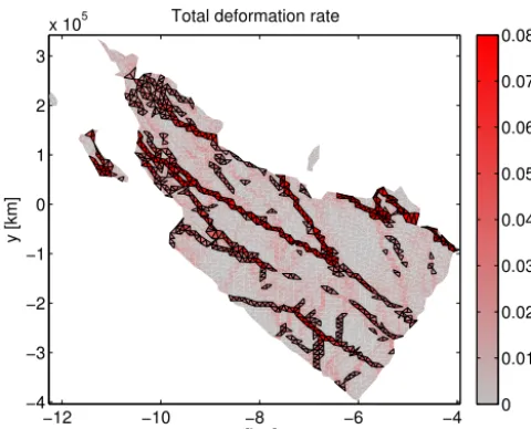
To apply the smoother, we first need to detect the cells that are suspected to map the location of linear kinematic fea-tures. Thomas et al. (2008) proposed using a threshold for the shear based on the level of noise resulting from the motion tracking error. Instead, here we use a fixed threshold based on the total deformation (as in the simple test case presented above) to give more weight to the cracks suffering from artifi-cial divergence. Cells showing total deformation greater than the threshold are thus selected and others simply not taken into account for the filtering procedure. Figure 5 shows the unfiltered total deformation rate and the selected cells (those with their edges in black) for a threshold equal to 0.02 per day.
−12 −10 −8 −6 −4 x 10⁵ −4
−3 −2 −1 0 1 2 3
x 105
x [km]
y [km]
Total deformation rate
[/day]
0 0.01 0.02 0.03 0.04 0.05 0.06 0.07 0.08
Figure 5. Unfiltered total deformation rate for the same example
as in Fig. 4. Triangles in black are above the threshold for the total deformation (here, 0.02 per day) and are then selected to be treated by the smoother.
smoother is not efficient anymore. Indeed if a kernel only contains one cell, the smoother does not modify the value of the deformation over that cell.
To quantify the effect of this threshold on the quality of the selection, we define an index based on the size of the smoothing kernels|Ks|(i.e., the number of cells that can be reached by crossing only selected cells and a maximum ofn edges). As explained in Sect. 2.1, the size of the kernel|Ks| could be as low asn+1 for single cracks when the center of the kernel is at the boundary of the mesh and as high as 4n+1 for two intersecting cracks. We then define the quality index as the percentage of treated cells having a kernel size between n+1 and 4n+1. For the example of Fig. 5, the quality index is equal to 89 %.
We explored the sensitivity of this quality index to the threshold value for the entire winter season 2006–2007 and with the parameternequal to 3, which is the reference value defined in Sect. 2.1. For deformation thresholds equal to 0, 0.01, 0.02, 0.03, 0.04 and 0.05 per day, median quality in-dices are equal to 33, 78, 78, 76, 74 and 72 %, respectively. Based on this quality index, the threshold values 0.01 and 0.02 per days are the best. The value of 0.02 per day is cho-sen as the reference value for the deformation threshold. To quantify the range of the quality index obtained with this ref-erence value, we look at the percentage of pairs of images for the entire winter 2006–2007 for which the quality index is lower than 50 %; our finding is that only 14 % of the pairs of images have a quality index lower than 50 %. To further vali-date the choice of the model parameters, a metric on a multi-fractal scaling analysis of the deformation fields is proposed in Sect. 3.
−12 −10 −8 −6 −4
x 105
−4 −3 −2 −1 0 1 2 3
x 105
x [km]
y [km]
Divergence rate
[/day]
−0.04 −0.03 −0.02 −0.01 0 0.01 0.02 0.03 0.04
Figure 6. Filtered divergence rate after the application of the
smoother to the selected cells (see Fig. 5). In this example, the pa-rameternis set to 3. The triangles that have been treated by the smoother are those in black in Fig. 5. For the other triangles, the value of the deformation remains the same as in Fig. 4.
Figure 6 shows the sea ice divergence field after the ap-plication of the smoother with the parametern equal to 3. Compared to the unfiltered divergence field shown in Fig. 4, the filtered field exhibits much less artificial noise and its in-terpretation is now much easier.
3 Results and discussion
In this section, we compare the original RGPS deformation data to the unfiltered and filtered versions of our RGPS Image Pair data set. A consistency check based on spatial scaling analysis is proposed and the differences between the three data sets in terms of spatial scaling and total opening/closing are discussed.
To compare the original RGPS deformation data with the unfiltered and filtered deformation data produced by our method, we generate composite pictures of the deformation rates for specific periods. The periods have to be long enough to ensure a good spatial coverage but not too long so as to avoid mixing incoherent information. For this study, we se-lect the data for which the time of the first and second images – notedtk−1andtk, respectively – are within a period of 8
−2500 −2000 −1500 −1000 −500 0 −500
0 500 1000 1500 2000
km from the pole
km from the pole Divergence rate in /day (kwok)
−0.04 −0.03 −0.02 −0.01 0 0.01 0.02 0.03 0.04
Figure 7. Composite picture of the divergence rate given by the
RGPS deformation data set for the period 2–10 February 2007. RGPS cells are here represented by squares as their actual shape is not known.
date, defined as(tk+tk−1)/2, is the closest to the target date. This selection step creates some gaps in the coverage but is necessary to ensure a minimum consistency of the composite fields. Note that no averaging or interpolation is done during the generation of the composite deformation fields.
Figure 7 shows the divergence rate for the period 2– 10 February 2007 given by the RGPS Lagrangian deforma-tion data set. Some features are so polluted by a succession of highly negative and positive values that it is very diffi-cult to identify where cracks are opening, closing or sliding. Figure 8 shows the unfiltered divergence rate for the same period obtained after the first step of our method. As in the RGPS data set, the artificial noise is important and mainly located along linear kinematic features. Figure 9 shows the filtered divergence rate obtained with a deformation thresh-old of 0.02 per day and n=3. The reduction of the noise makes much easier the identification of the opening and clos-ing cracks.
3.1 Consistency check
To evaluate our method in a more quantitative way, we pro-pose a metric based on a spatial scaling analysis. Scaling analysis is a powerful tool to characterize sea ice dynamical behavior and has been successfully used in previous stud-ies to reveal the power-law scaling of sea ice deformations (Marsan et al., 2004; Rampal et al., 2008).
The spurious noise in the deformation fields corresponds to high values of deformation and is potentially present for any active linear kinematic features. This noise may then impact the distributions of shear and absolute divergence and modify their mean (first-order moment) but even more their standard deviation (second-order moment) and
skew-−2500 −2000 −1500 −1000 −500 0
−500 0 500 1000 1500 2000
km from the pole
km from the pole Divergence rate in /day (unfiltered)
−0.04 −0.03 −0.02 −0.01 0 0.01 0.02 0.03 0.04
Figure 8. Composite picture of the unfiltered divergence rate
com-puted after the first step of our method for the period 2–10 February 2007.
−2500 −2000 −1500 −1000 −500 0
−500 0 500 1000 1500 2000
km from the pole
km from the pole Divergence rate in /day (filtered)
−0.04 −0.03 −0.02 −0.01 0 0.01 0.02 0.03 0.04
Figure 9. Composite picture of the filtered divergence rate for the
period 2–10 February 2007 obtained with a threshold parameter equal to 0.02 per day and with the parameternequal to 3.
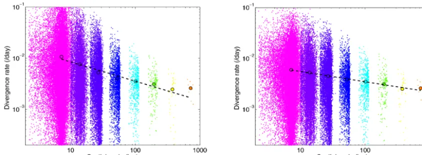
Figure 10. Scaling analysis: absolute divergence rate as a function of the spatial scale, from the unfiltered (left panel) and filtered (right
panel) composite deformation field for the period 2–10 February 2007 (each color corresponds to a different box size used for the coarse graining procedure). The mean valuesh| ˙div|iare represented by circles, and the dashed lines are power-law fits of the first six mean values
(here, from 7 to 200 km)
power-law model when approaching the spatial resolution of the data could be seen as an indicator of the remaining noise in the deformation field.
To perform the scaling analysis of sea ice deformation, we implemented a coarse graining method similar to the one pro-posed by Marsan et al. (2004) and applied it to the unfiltered and filtered versions of our RGPS Image Pair data set. Sea ice shear and absolute divergence rates are computed at different spatial scales ranging from 7 to 700 km. For the lowest scale, which is also the scale of the triangular cells, all the cells are taken into account. For the other scales, the coarse graining procedure covers the domain with boxes of different sizes (14, 28, 56, 112, 224, 448 and 896 km). The boxes actually overlap since a distance equal to half the box size separates their respective centers. For each box, we select the cells that have their center in the box. When the sum of the area of those cells is greater than half the box area, the deformation over the box is defined by averaging the spatial derivatives of the displacement weighted by the surface of each cell. The spatial scale for this new estimate of the deformation is the square root of the sum of the cell areas. The shear and abso-lute divergence for each box are then reported as a function of the spatial scale on a log–log plot (see Fig. 10 for the abso-lute divergence rate). The mean valueh ˙Li(where˙Lis either
the shear rates or the absolute divergence rates, computed at scaleL) relates to scaleLfollowing a power law. The power-law exponent is evaluated by applying a linear regression of the logarithm ofh ˙Livs. the logarithm ofL. Due to the
fi-nite size of the domain the power-law model is not expected to hold for the largest scales. For this reason we restrict the power-law regression of the data to the spatial scales 7, 14, 25, 50, 100 and 200 km.
The filtered shear and absolute divergence closely follow the power-law model for the spatial scaling as their first-order moments are well aligned with the power-law fit for
the spatial scales ranging from 7 to 200 km (see right panel of Fig. 10 for the absolute divergence). This is not the case for the unfiltered deformation fields (see left panel of Fig. 10), and we explain this strong departure from the power-law model by the presence of artificial noise. If the power-law fits were computed only from 50 to 200 km, spatial scaling ex-ponents would be similar for the filtered and unfiltered data. Furthermore, the other momentsh ˙Lqiof the distributions (see Fig. 11 for the absolute divergence rate, withq, the moment order, ranging from 0.5 to 3) computed from the unfiltered deformation fields also exhibit a strong departure from the power law, whereas the moments computed from the filtered deformation fields are well aligned with the power-law fits.
By definition, if a scaling holds for a given range of scales, it should be respected for any pair of scales within this range. To evaluate the deviation from the power-law scaling, we compute the power-law exponents for each pair of succes-sive spatial scales (i.e., from 7 to 14 km, from 14 to 25 km, and so on) and we take the minimum and maximum values of these exponents. Those values as well as the exponents previously obtained with the whole range from 7 to 200 km are reported as a function of the moment orderq in Fig. 12. The relationship between the power-law exponents and the moment orderq is called the structure functionβ(q)and is defined byh ˙Lqi ∼L−β(q). The minimum and maximum ex-ponents define the bars aroundβ(q).
10 100 1000 10−8
10−6 10−4 10−2
Mean divergence rate (/day)
Spatial scale (km) 10 100 1000
10−8 10−6 10−4 10−2
Mean divergence rate (/day)
Spatial scale (km)
q = 1
q = 0.5
q = 1.5
q = 2
q = 2.5
q = 3
Figure 11. Multifractal analysis: moments of the absolute divergence ratesh| ˙div|qias a function of the scaleLforq=0.5 to 3, from the
unfiltered (left panel) and filtered (right panel) composite deformation field for the period 2–10 February 2007. Dashed lines are power-law fits of the first six values (here, from 7 to 200 km).
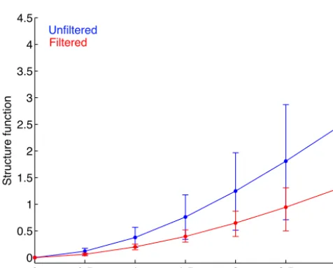
0 0.5 1 1.5 2 2.5 3
0 0.5 1 1.5 2 2.5 3 3.5 4 4.5
Structure function
Moment order q
Unfiltered
Filtered
Figure 12. Structure functionβ(q)corresponding to the exponents of the power-law relationship between the absolute divergence rate and the spatial scale: h| ˙div|qi ∼L−β(q). The bars on the graph
indicate the deviation from the power law as they correspond to the minimum and maximum power-law exponents obtained for two successive spatial scales.
of 0.02 per day gives the lowest min–max error for the high-est order. For the parametern, the lowest min–max error for the highest moment order is obtained withn=2, butn=3 is better for the other moment orders. The application of our metric to this single example tends to indicate that the refer-ence values are well chosen. However, this metric should be applied to a larger number of examples to really identify the best values for the parameters.
3.2 Discussion
Comparing the original RGPS deformation to the unfiltered deformation allows us to evaluate the impact of using a trian-gulation to define well-shaped triangular cells. As in Lindsay and Stern (2003), we observe unrealistic values for the shear and divergence rates retrieved from the RGPS deformation data set. For the period 2–10 February 2007, the composite picture made from RGPS has maximum opening, closing and shear rates equal to 1.73,−6.73 and 66.47 per day, respec-tively. These extreme values arise from highly distorted cells. A very small fraction of the data set is polluted by these unre-alistic values; however it has a high impact on the multifrac-tal scaling analysis, particularly when looking at the highest moment orders of the distributions. In Marsan et al. (2004) and Stern and Lindsay (2009), additional constraints on the initial and current size of the cells were applied and the cells with total deformation higher than 1 per day were not taken into account. In many other studies based on the RGPS defor-mation data set, the presence and impacts of these unrealistic extreme values are simply not discussed.
The simple fact of redefining a new mesh from the actual position of the RGPS nodes allows us to avoid badly shaped cells and then to significantly reduce the number and magni-tude of extreme values. For the same period, the composite picture obtained from the unfiltered version of our RGPS Im-age Pair data set has maximum opening, closing and shear rates equal to 0.63, −1.17 and 1.97 per day, respectively. The smoother also logically decreases the extreme values. For this example, the filtered composite picture has maxi-mum opening, closing and shear rates equal to 0.13,−0.20 and 0.73 per day, respectively.
-0.1 -0.2 -0.3 -0.4
-0.5 10−4 0.1 0.2 0.3 0.4 0.5
10−3 10−2 10−1 100 RGPS
Unfiltered Filtered
Divergence rate (/day)
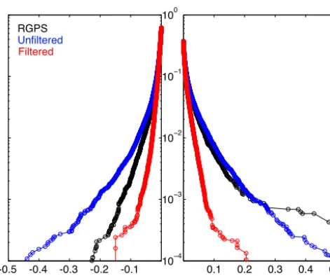
Figure 13. Cumulative probability functions – in other words, the
probabilities of exceedance – for the RGPS, unfiltered and filtered composite divergence fields shown in Figs. 7–9, respectively.
from the unfiltered fields are systematically larger in mag-nitude by about 100 % for the absolute divergence and by about 50 % for the shear and total deformation. In the exam-ple corresponding to Fig. 10, the power-law exponent for the absolute divergence is−0.38 for the unfiltered field, instead of −0.20 for filtered data (for the shear: −0.17 instead of
−0.1; for the total deformation:−0.19 instead of−0.12). For each moment, we observe that using unfiltered data leads to a systematic overestimation of the scaling exponents of about 100 % for the absolute divergence and 50 % for the shear and total deformation. We also performed the multifractal scaling analysis on the original RGPS deformation data set with the same constraints on the data as in Stern and Lindsay (2009), and we found that the departure from the power law is similar to the one observed for the unfiltered deformation data set.
The impact of the artificial noise is also seen on the struc-ture function β(q) (see Fig. 12). As a consequence of the systematic overestimation of the scaling exponents, its cur-vature, which indicates the degree of multifractality of the deformation fields, is found to be twice as high for the unfil-tered divergence field (0.20) than for the filunfil-tered one (0.11). For the shear and total deformation, the overestimation of the curvature is about 50 %, with a value of 0.16 instead of 0.1.
Differences are also seen in the cumulative distribution of the closing and opening rates (see Fig. 13 for the period 2– 10 February 2007). Differences between the RGPS and the unfiltered deformation may be due to differences in the cov-erage and the selection of the data, but they also come from the difference in resolution (10 km for the RGPS instead of 7 km) and from the impact of distorted cells included in the RGPS data set. Differences between the filtered and unfil-tered deformation induce a modification of the shape of the distribution. The distribution of the filtered divergence field
is closer to an exponential distribution (linear in the semi-log plot), while the distribution of the unfiltered divergence field is clearly a stretched exponential.
Finally, we compare the three data sets by computing the total area that has been opened and closed. For the orig-inal RGPS deformation data, 40 000 km2 has been opened during the period 2–10 February 2007, whereas 39 000 km2 have been closed. For our unfiltered data, we find lower values of 30 000 and 38 000 km2, respectively. For the fil-tered data these numbers drastically drop down to 15 000 and 24 000 km2, respectively. In this example the artificial noise is thus responsible of an overestimation of the opening and closing of about 100 and 60 %, respectively. Over the entire winter season 2006–2007, the cumulative opening and clos-ing are both 60 % higher in the unfiltered data than in the filtered data.
4 Conclusions
A method is proposed to derive accurate sea ice deformation fields from SAR-derived motion products. The first step of the method consists of a triangulation of the tracked points to generate a mesh of triangular cells on which a first estimate of deformation is computed. The second step consists of ap-plying a smoother to the deformation fields. The method re-lies on two parameters: a deformation threshold and the size of the smoothing kernel.
By applying the method to idealized test cases, we show that using triangles instead of quadrangles induces an in-crease of only about 10 % of the opening and closing er-ror, whereas our smoothing method reduces the opening and closing error by at least a factor of 3 in any of the test cases presented here. The sensitivity to the value of the threshold used to detect deformation features is analyzed with a qual-ity index, and the efficiency of our method is assessed using a metric based on a spatial scaling analysis and comparison between the unfiltered and filtered deformation fields.
The proposed method is used to produce a new deforma-tion data set called RGPS Image Pair Product. Compared to the RGPS deformation data set, the RGPS Image Pair data set does not exhibit unrealistic large values caused by badly shaped cells. Moreover, our method drastically reduces the artificial noise arising along dynamic discontinuities.
By comparing the unfiltered and filtered deformation fields for winter 2006–2007, we estimate that this artificial noise may cause an overestimation of the opening and closing of about 60 %. We also estimate that the spatial scaling expo-nents as computed in Marsan et al. (2004) and Stern and Lindsay (2009) could have been overestimated by about 100 % for the absolute divergence and by about 60 % for the shear and total deformation.
po-tential significant biases on the estimates of sea ice produc-tion, salt rejection and sea ice ridging that one may find in the literature.
The method proposed here is applicable to other sea ice drift data sets, as provided, for example, by the GlobICE project. The method can handle Lagrangian trajectories or displacement between pairs of images. The same method could be applied to buoy trajectories when their spatial reso-lution is high enough, as with nested arrays of buoys (Hutch-ings et al., 2011, 2012).
The method proposed here could be modified to better manage intersecting cracks and to adapt its parameters de-pending on the local fields. However, substantial improve-ments may also come by combining, within tracking algo-rithms, the detection of dynamic discontinuities and the com-putation of sea ice deformation as proposed by Thomas et al. (2008). A complete validation using independent data sets should also be carried out.
Acknowledgements. S. Bouillon is supported by the Research
Council of Norway through the post-doc project SIMech, Sea Ice Mechanics: from satellites to numerical models (no. 231179/F20, 2014–2016). P. Rampal is supported by the Kara Sea project sponsored by Total E&P. Many thanks to Tim Williams and Gunnar Spreen for interesting discussions.
Edited by: D. Feltham
References
Bremner, D., Hurtado, F., Ramaswami, S., and Sacristán, V.: Small convex quadrangulations of point sets, in: Algorithms and Com-putation, edited by: Eades, P. and Takaoka, T.: of Lecture Notes in Computer Science, Springer Berlin Heidelberg, 2223, 623– 635, doi:10.1007/3-540-45678-3_53, 2001.
Fily, M. and Rothrock, D.: Opening and closing of sea ice leads: digital measurements from synthetic aperture radar, J. Geophys. Res., 95, 789–796, 1990.
Girard, L., Weiss, J., Molines, J.-M., Barnier, B., and Bouillon, S.: Evaluation of high-resolution sea ice models on the basis of sta-tistical and scaling properties of Arctic sea ice drift and deforma-tion, J. Geophys. Res., 114, 2156–2202, 2009.
Girard, L., Bouillon, S., Weiss, J., Amitrano, D., Fichefet, T., and Legat, V.: A new modelling framework for sea ice mechanics based on elasto-brittle rheology, Ann. Glaciol., 52, 123–132, 2011.
Herman, A. and Glowacki, O.: Variability of sea ice deformation rates in the Arctic and their relationship with basin-scale wind forcing, The Cryosphere, 6, 1553–1559, doi:10.5194/tc-6-1553-2012, 2012.
Hollands, T. and Dierking, W.: Performance of a multiscale cor-relation algorithm for the estimation of sea-ice drift from SAR images: initial results, Ann. Glaciol., 52, 311–317, 2011. Hutchings, J. K., Roberts, A., Geiger, C. A., and Richter-Menge, J.:
Spatial and temporal characterization of sea-ice deformation, Ann. Glaciol., 52, 360–368, 2011.
Hutchings, J. K., Heil, P., Steer, A., and Hibler III, W. D.: Subsyn-optic scale spatial variability of sea ice deformation in the west-ern Weddell Sea during early summer, J. Geophys. Res., 117, C01002, doi:10.1029/2011JC006961, 2012.
Kwok, R.: The RADARSAT Geophysical Processor System, in: Analysis of SAR data of the Polar Oceans: Recent Advances, edited by: Tsatsoulis, C. and R. Kwok, Springer Verlag, 235– 257, 1998.
Kwok, R.: Contrasts in sea ice deformation and production in the Arctic seasonal and perennial ice zones, J. Geophys. Res., 111, C11S22, doi:10.1029/2005JC003246, 2006.
Kwok, R. and Cunningham, G. F.: Seasonal ice area and volume production of the Arctic Ocean: Novem-ber 1996 through April 1997, J. Geophys. Res., 107, 8038, doi:10.1029/2000JC000469, 2002.
Kwok, R., Curlander, J. C., McConnell, R., and Pang, S. S.: An Ice Motion Tracking System at the Alaska SAR Facility, IEEE J. Ocean. Engin., 15, 44–54, 1990.
Kwok, R., Rothrock, D. A., Stern, H. L., and Cunningham, G. F.: Determination of the age distribution of sea ice from Lagrangian observations of ice motion, IEEE T. Geosci. Remote, 33, 392– 400, 1995.
Kwok, R., Hunke, E. C., Maslowski, W., Menemenlis, D., and Zhang, J.: Variability of sea ice simulations assessed with RGPS kinematics, J. Geophys. Res., 113, 2156–2202, 2008.
Lindsay, R. W. and Stern, H. L.: The RADARSAT geophysical pro-cessor system: quality of sea ice trajectory and deformation esti-mates, J. Atmos. Ocean. Tech., 20, 1333–1347, 2003.
Lindsay, R. W., Zhang, J., and Rothrock, D. A.: Sea-ice deformation rates from satellite measurements and in a model, Atmos. Ocean, 41, 35–47, doi:10.3137/ao.410103, 2003.
Marsan, D., Stern, H. L., Lindsay, R., and Weiss, J.: Scale depen-dence and localization of the deformation of Arctic sea ice, Phys. Rev. Lett., 93, 178501–178504, 2004.
Rampal, P., Weiss, J., Marsan, D., Lindsay, R., and Stern, H. L.: Scaling properties of sea ice deformation from buoy dispersion analysis, J. Geophys. Res., 113, C03002, doi:10.1029/2007JC004143, 2008.
Stern, H. L. and Lindsay, R.: Spatial scaling of Arctic sea ice deformation, J. Geophys. Res., 114, C10017, doi:10.1029/2009JC005380, 2009.
Thomas, M., Geiger, C. A., and Kambhamettu, C.: High resolution (400 m) motion characterization of sea ice using ERS-1 SAR im-agery, Cold Reg. Sci. Technol., 52, 207–223, 2008.
Thorndike, A. S.: Kinematics of Sea Ice, in: The Geophysics of Sea Ice, NATO ASI Series, edited by: Untersteiner, N., Plenum Press, New York, 489–549, 1978.