www.atmos-meas-tech.net/6/2851/2013/ doi:10.5194/amt-6-2851-2013
© Author(s) 2013. CC Attribution 3.0 License.
Atmospheric
Measurement
Techniques
Semi-autonomous sounding selection for OCO-2
L. Mandrake1, C. Frankenberg1, C. W. O’Dell2, G. Osterman1, P. Wennberg3, and D. Wunch3 1Jet Propulsion Laboratory, California Institute of Technology, Pasadena, CA, USA
2Colorado State University, Fort Collins, CO, USA 3California Institute of Technology, Pasadena, CA, USA
Correspondence to: L. Mandrake ([email protected])
Received: 10 June 2013 – Published in Atmos. Meas. Tech. Discuss.: 26 June 2013
Revised: 13 September 2013 – Accepted: 23 September 2013 – Published: 25 October 2013
Abstract. Many modern instruments generate more data than may be fully processed in a timely manner. For some atmo-spheric sounders, much of the raw data cannot be processed into meaningful observations due to suboptimal viewing con-ditions, such as the presence of clouds. Conventional solu-tions are quick, empirical-threshold filters hand-created by domain experts to weed out unlikely or unreasonable obser-vations, coupled with randomized down sampling when the data volume is still too high. In this paper, we describe a method for the construction of a subsampling and ordering solution that maximizes the likelihood that a requested data subset will be usefully processed. The method can be used for any metadata-rich source and implicitly discerns informa-tive vs. non-informainforma-tive data features while still permitting user feedback into the final features selected for filter imple-mentation. We demonstrate the method by creating a selector for the spectra of the Japanese GOSAT satellite designed to measure column averaged mixing ratios of greenhouse gases including carbon dioxide (CO2). This is done within the
At-mospheric CO2Measurements from Space (ACOS) NASA
project with the intention of eventual use during the early Orbiting Carbon Observatory-2 (OCO-2) mission. OCO-2 will have a 1.5 orders of magnitude larger data volume than ACOS, requiring intelligent pre-filtration.
1 Introduction
Atmospheric composition measurement, like so many mod-ern disciplines, is undergoing a radical transformation due to new sensors. Ultra-high data rate, computerized instruments operate at hyper-spectral resolutions from space-borne plat-forms that operate over land and sea, day and night. Each
data point was once a precious commodity carefully con-sidered by multiple researchers; now an individual is swiftly presented with millions of observations and their associated metadata. A key challenge to handling the increased data vol-ume is the estimation of data quality, to prevent the waste of precious human attention. Many remotely sensed atmo-spheric data suffer from unavoidable confounding aspects such as cloud cover or aerosols yielding distorted or unus-able results given current retrieval algorithms. Certain ob-serving conditions may a priori pose known problems for the processing algorithm, e.g. bright icy surfaces, dark oceans, or the complex surfaces of mountains (O’Dell et al., 2012). The instrumentation also contributes to difficulty in main-taining data quality, with drifting calibration, reset events, detector saturation or low-level preprocessor version changes making evaluation difficult. Poorly modeled physical pro-cesses also act as confounding forces in the observations where they dominate over the intended measurement the-ory during retrieval processing. When the data set is small, manual filtering of the data based on expert knowledge and past experience is a time-tested method for evaluation. But when millions of observations are faced, we must resort to an automated rules-based filtration without the advantage of personal interaction with each sounding.
scientist then looks for thresholds in these candidate filtra-tion features, beyond which the values change from reason-able to unreasonreason-able based on prior knowledge, and visual features in the graph of feature versus desired output. A key question is how one knows the reasonable from the unrea-sonable, with the answer that only in rather egregious cases is the answer clear.
The resultant filter, often constructed from the amalgam of many “reasonability” thresholds, produces a cleansed data set that has flagged as questionable much of the obviously flawed data outliers. Some iteration is then performed by manually modifying the individual “reasonability” thresh-olds to alter the percentage of data passage to match the immediate needs of the project. This yields a final “fixed” filter with a given throughput and performance. The lack of ability to tune the filter in real time to increase or decrease throughput is one major shortcoming of such filters, as is the complexity of decoding why a particular data point has been excluded given several interacting potential filtration rules.
Generally, few scientific data sets are dominated by data that is entirely corrupt or acceptable. Instead, shades of ac-ceptability for any particular data result from varying de-grees of influence from confounding forces. Instead of con-structing a binary good/bad filter, we observe the opportu-nity for a well-constructed data-screening algorithm: the or-dering of the data by the statistical likelihood of each obser-vation’s scientific utility. Such an ordering could reproduce the above fixed filter performance by fixing the percentage of acceptance; beyond this, it permits the variation of the data passage rate in real time in a principled manner. In or-der to construct an estimate of a given observation’s reliabil-ity, we turn to machine learning to emulate the same manual filter-construction process researchers traditionally perform on smaller data sets. By automatically constructing an en-semble of traditional, fixed filters, we may construct an esti-mate of the reliability of each data point based on the number of fixed filters that would reject it. It is important to recall we are describing a process that provides a robust, tunable filter, not merely a single static filter suggestion.
The satellite mission driving our development of new data filtering techniques is the Orbiting Carbon Observatory-2 (OCO-2) set to launch in 2014 with the intention of mak-ing atmospheric carbon dioxide (CO2)measurements (Crisp
et al., 2004; Connor et al., 2008; Boesch et al., 2011; O’Brien et al., 2011). OCO-2 will generate 24 soundings per sec-ond with each sounding comprised of∼3000 spectral radi-ance measurements, placing it soundly in the large data limit. The sophisticated physics-based retrieval algorithm (O’Dell et al., 2012) requires approximately 10 CPU minutes (3 GHz Intel Xeon) to render each spectrum into a single retrieved Level 2 column CO2 value. This data volume will outpace
real-time processing for anything less than ∼14 000 CPU cores, ignoring scaling inefficiencies that would increase the challenge. Even taking into account progress made to reduce the runtime of the OCO-2 Level 2 code as well as advances in
hardware capability in advance of the expected 2014 launch date, selecting the “right” data to process will be critical. To satisfy the mission requirement that at least 6 % of the sound-ings be processed in real time, it is likely that we must intel-ligently pre-select the soundings we attempt to process. This pre-selection of data with the highest scientific interest and minimal confounding influence is the definition of the sound-ing selection problem. We further wish to ensure we provide sampling criteria that maximize the utility of the OCO-2 data for estimation of carbon fluxes – the raison d’etre for the observatory. For instance, it is crucial that we sample CO2
at many atmospheric temperatures, pressures, seasons, and across many different Earth surface types, even if the cur-rent retrieval algorithm struggles in a region defined by such features.
2 Data: GOSAT/ACOS example, pre-processing, features used
In order to develop and test a method of sounding selector creation for the future OCO-2 mission, we use measurements of carbon dioxide taken by the Greenhouse gases Observ-ing SATelite (GOSAT) provided by a joint effort between the Japanese Exploration Agency (JAXA), the Japanese National Institute for Environmental Studies (NIES) and the Japanese Ministry of the Environment (MOE). GOSAT measures in the same spectral regions as OCO-2 and provides a test bed for the OCO-2 retrieval algorithm (Yokota et al., 2004). The Atmospheric CO2 Observations from Space (ACOS)
project creates a global carbon dioxide data product from the GOSAT observations. Processing the GOSAT soundings in-formed OCO-2 software development while the instrument was being built and integrated onto the spacecraft. We utilize ACOS/GOSAT soundings taken between 6 April 2009 and 30 September 2010, resulting in a set of 4.8 million sound-ings. We take only data recorded in the GOSAT “high gain” mode (Wunch et al., 2011; Crisp et al., 2012), as it is the dominant data type in number (86 %) and global coverage.
While the OCO-2 Level 2 retrieval software is used on the GOSAT data to generate the ACOS data set, the GOSAT L1 metadata is utilized directly, consisting of geospatial infor-mation and estimates of signal-to-noise provided by JAXA. The L1 radiance spectra are not directly used for developing a sounding selection scheme, but are used in retrieval pre-processing routines that then feed into the sounding selector. The L1 data are used in a cloud detection scheme (Taylor et al., 2012) and a combination cloud filter and CO2quick-look
24 1
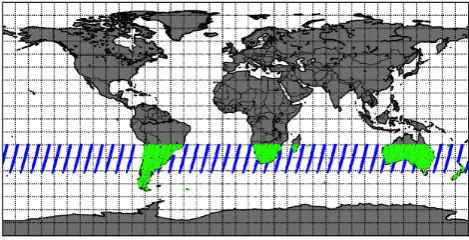
Figure 1. The land and sea data used in the southern hemisphere approximation. This region is 2
observed to have very low seasonal CO2 fluctuation relative to the north.
3 4
Fig. 1. The land and sea data used in the Southern Hemisphere
ap-proximation. This region is observed to have very low seasonal CO2
fluctuation relative to the north.
independent regions of the radiance spectrum. Finally, some statistical measurements of the radiance spectra are also cal-culated such as standard deviation, max, min, and mean. To-gether, these form the metadata and metric inputs (features) that we will use to divine a sounding’s likelihood of being successfully retrieved. Table 1 shows the quantity, type and origin of the features used.
To guide our filter optimization, we seek to minimize the scatter in the final retrieved CO2 value produced by the
full physics retrieval algorithm (here version B2.10), after the official cloud filtration algorithm has been applied (see Sect. 3.2.2). We focus on the low variation of atmospheric CO2in the Southern Hemisphere (20◦to 60◦S, see Fig. 1).
Applying these criteria results in 40 000 retrievals over land and 24 000 over ocean for training purposes.
3 Method: hyper-dimensional filter, goal function, and genetic algorithm
In this section we provide an overview of the methods to be used in the general case. We start by defining a large set of filters similar to those produced by experts. Each of these filters may use information from sounding metadata (a pri-ori surface pressure and temperature, etc.) or direct spectral measurements (e.g. SNR, band ratios, etc.). We then utilize a genetic algorithm to optimize the thresholds of these fil-ters, seeking to minimize the scatter in the retrieved CO2in
the Southern Hemisphere while maximizing the amount of data passed and minimizing the number of rules required in each filter. We produce 20 “warn levels” from 19 represen-tative filters that summarize each sounding’s acceptability to the larger set of filters, where a high warn level predicts most filters would reject a given sounding. The warn levels, in ad-dition to spatial coverage requirements, form the basis of the sounding selector itself. The specific implementation of these methods is provided in Sect. 4 for the GOSAT B2.10 data set.
25 1
Figure 2. Two-dimensional feature example. Yellow lines represent the max and min 2
thresholds for each of the two sub-filters, with only data satisfying the union (green) accepted 3
by the filter and all other data (red) rejected. 4
5
Fig. 2. Two-dimensional feature example. Yellow lines represent
the max and min thresholds for each of the two subfilters, with only data satisfying the union (green) accepted by the filter and all other data (red) rejected.
3.1 Hyper-dimensional filter
Following the “human expert” model of filter construction, we define a fixed filter as the union of a large number of sim-ple threshold cutoffs (subfilters) each defined by a maximum and minimum threshold value beyond which data will be re-jected (Fig. 2). One such subfilter is required for each in-put feature. Optimizing the high and low threshold for each subfilter defines the fixed filter creation problem, and the en-tire list of thresholds (number of input features×2) uniquely defines a fixed filter and is a high dimensional parameter space. A human expert generally creates one or two fixed filters, with the goal of segregating high, medium, and poor data quality or simply pass and fail. The full sounding selec-tor will be based on an ensemble of 19 fixed filters, each with their own optimized subfilters. A guiding diagram is provided in Fig. 3.
3.2 Genetic algorithm
Table 1. Features considered as input to the GOSAT sounding selector construction.
Quantity Type Example Source
8 Physical Tsurf,Psurf Cloud Filter Pre-process
5 Signal Characteristics SNR Cloud Filter Pre-process 5 Physical CO2density IMAP-DOAS Pre-process 12 Spectral Stats Stdev(radiance) Spectral math on radiance spectra 30 Signal Characteristics SNR JAXA
43 Geometry Azim, Alt, fractionland JAXA
103 Total
26 1
Figure 3. A guiding diagram for the discussion of filters and the final sounding selector. Note 2
that the double “Low, High” thresholds in the upper right table show that each of the Warn 3
Levels is crafted from the combination of more than one Fixed Filter (in this example, two). 4
Thus, two low and two high thresholds will be required given two input features. The 5
colorscale in the Desired Spatial Coverage to the lower left indicates the user-specified 6
sounding density in each bin. 7
8
Fig. 3. A guiding diagram for the discussion of filters and the final
sounding selector. Note that the double “Low, High” thresholds in the upper right table show that each of the Warn Levels is crafted from the combination of more than one Fixed Filter (in this exam-ple, two). Thus, two low and two high thresholds will be required given two input features. The color scale in the Desired Spatial Cov-erage to the lower left indicates the user-specified sounding density in each bin.
3.2.1 Gene
The first step of defining a GA is formulating the parame-ters (gene) that encapsulate the problem to be solved. In our case, we use the full list of subfilter high and low thresh-olds defined in Sect. 3.1 along with a Boolean list of whether each subfilter is actively being used. This list will permit us to track and control how many subfilters are actually used in each fixed filter, with the total number of active subfilters called a fixed filter’s complexity. Initially, we start with a fil-ter that permits all data and uses no active subfilfil-ters, thus complexity=0. A gene that only had two subfilters switched on would be complexity 2, and all subfilters active would result in a complexity equal to the total number of features. Fixed filters constructed by humans are often highly complex by this definition, as they can have dozens of active subfilters.
27 1
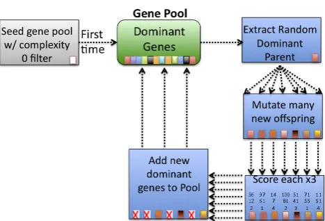
Figure 4. The genetic algorithm (GA) cycle. A parent is selected from the dominant gene 2
pool, mutated into thousands of offspring, and any new dominant solutions are added back 3
into the pool while the others are discarded. This cycle can be run massively in parallel, with 4
each process contributing to the same ever-improving gene pool. 5
6
Fig. 4. The genetic algorithm (GA) cycle. A parent is selected from
the dominant gene pool, mutated into thousands of offspring, and any new dominant solutions are added back into the pool while the others are discarded. This cycle can be run massively in parallel, with each process contributing to the same ever-improving gene pool.
3.2.2 Fitness & goal function
Next we define the fitness by which each proposed genetic solution is judged. This, coupled with the definition of the gene in Sect. 3.2.1, fully defines the problem. Optimally, we would attempt to minimize the RMS difference between our retrieved L2 CO2values and the true CO2value over the
en-tire globe across many years. Global CO2observations from
satellites exist but are not ideal for comparison to ACOS data and high quality surface data are spatially sparse (Wunch et al., 2011; Reuter et al., 2011). Instead, we utilize the South-ern Hemisphere approximation: the annual CO2variation of
the Southern Hemisphere appears to be relatively small and reasonably approximated by a secular trend (linear yearly increase) with a very small sinusoidal seasonal component (Wunch et al., 2011). Most of the scatter seen in the South-ern Hemisphere ACOS data is most likely caused by con-founding forces negatively affecting the retrieval algorithm rather than actual CO2fluctuation (Wunch et al., 2011). This
28 1
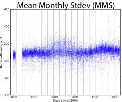
Figure 5.A heat map of the retrieved values of CO2 for the entire southern hemisphere over 2
land is shown. The blue bars identify the monthly bins within which the standard deviation 3
will be taken. The MMS is the mean of each of the standard deviations of these 18 bins. 4
5
Fig. 5. A heat map of the retrieved values of CO2for the entire
Southern Hemisphere over land is shown. The blue bars identify the monthly bins within which the standard deviation will be taken. The MMS is the mean of each of the standard deviations of these 18 bins.
that creating a filter using TCCON comparison or Southern Hemisphere approximation yields extremely similar results.
We create a metric called mean monthly standard devia-tion (MMS):
MMS=
P
monthly_bins
Stdev(CO2)
num_monthly_bins , (1)
where only monthly bins with more than ten soundings are admitted into the above average (see Fig. 5 for a graphical example). Measured in parts per million (PPM), the same unit as CO2, it represents an overall scatter for the entire set
of xCO2 measurement from ACOS in the Southern
Hemi-sphere. The monthly grouping is to avoid any minor seasonal oscillations present in the data as well as the increase in CO2.
Reducing the MMS through data filtration will be considered our primary goal.
The trivial solution to reduce MMS would be to filter all but a few very consistent soundings in a single monthly bin. In order to make this trade-off explicit, we will label fixed fil-ter solutions with the percentage of data passed through the filter (transparency). Measured to tenths of a percent, this be-comes a discrete quantity fundamental to the construction of our ensemble. Another goal will be to reduce the number of active subfilters necessary to achieve a solution or the com-plexity (also a discrete quantity). This allows for the preven-tion of overly complex fixed filters requiring dozens of subfil-ters when a very small number might perform almost as well. GA’s handle multiple goals like these gracefully through the concept of dominance, as discussed in the next section.
3.2.3 Dominance
When evaluating a new, proposed fixed filter’s fitness, we compute its MMS, transparency, and complexity. Trans-parency is resolved to 0.1 % resolution, resulting in 1000 bins for the full range of 0 to 100 %. We then compare its MMS to a small population of past most-fit solutions called the Gene Pool. Within the Gene Pool past solutions are grouped by the discrete labels of transparency and complexity, ranked by resulting MMS. Only if the new proposed fixed filter has a lower MMS for a given complexity and transparency does it dominate (replace) the prior solution and continue into the next generation. In this way, we are running thousands of si-multaneous races, 1000 transparency bins multiplied by the maximum complexity we will tolerate, that being 10 in the GOSAT example.
The net result of this process is not to find a single best fixed filter as a human expert might seek, but to form a pop-ulation of dominant solutions that cannot be further reduced without specifying preferences between the three fitness met-rics of transparency, complexity, and MMS. This population is known as the Pareto optimal front in machine learning cir-cles (Jin and Sendhoff, 2008). Instead of seeking to arbitrar-ily judge between these three conflicting goals, we will pre-serve the trade-off space of equally fit fixed filters to help satisfy other requirements of our overall filter solution such as spatial coverage and tunability.
3.2.4 Reproduction
stable, that is minimally changing from cycle to cycle, and we achieve Pareto optimality.
3.2.5 Termination
The GA is permitted to run until the known dominant filters in the gene pool do not substantially change, i.e. the MMS for any particular transparency and complexity reduces by less than 0.01 % per hundred GA cycles. In practice, this was a very stringent condition and looser definitions of termination would have resulted in similarly acceptable filter solutions. 3.3 Feature selection
Feature selection is the process of determining which of the input features are useful or informative for a given problem (Guyon and Elisseeff, 2003). In our example, we seek to an-swer which of the initial features aid us in minimizing the Southern Hemisphere scatter. The GA has produced several thousand dominant fixed filters that trade off MMS, trans-parency, and complexity. By examining the subset of the ini-tial features selected by the GA in these dominant filters, we create a list of known informative features. Those not se-lected are either redundant, containing the same information as the chosen set, or are uninformative.
As we did not a priori restrict the choice of data features, each fixed filter might (but likely does not) employ totally different features in its functioning even for small changes in performance metric. This is exacerbated by the presence of highly correlated or equivalent features in our input data, such as the altitude of a sounding using two differing Earth spheroid estimates or multiple estimates of surface pressure using differing assumptions. Though the GA considers such nearly equivalent features as interchangeable and will flut-ter between them from fixed filflut-ter to fixed filflut-ter, some are often more interpretable than others. For example, two fea-tures commonly interchanged are the SNR and the standard deviation of the radiance spectrum. The SNR is straightfor-ward to interpret, whereas the standard deviation of intensity convolves the SNR, overall brightness, and other more subtle quantities. Therefore, the set of informative features resulting from the GA is a superset that likely contains highly corre-lated, interchangeable features. We may take advantage of this apparent nuisance, hand-selecting out features from the GA-generated list that are (A) highly informative, (B) appear many times in the dominant fixed filters, and (C) are most interpretable. A second run of the GA would then be per-formed using only this fine-tuned list of desirable features, regenerating the full dominant population with improved in-terpretability and minimized interchangeable feature oscilla-tion. As such, this method is semi-autonomous rather than fully automatic, as human intervention has been permitted to aid in the fine-tuning and sanity checking of the features used in the final, dominant fixed filter solutions. However, the human expert in this case has already been aided by the
GA’s focus on informative features in a data-driven, empiri-cal manner.
3.4 Warn level
We now need a way to utilize the knowledge contained in the ensemble of dominant fixed filters. The human expert standard method would pick a single fixed filter that had the MMS reduction and transparency desired, using personal judgment to perform the balance between these goals. We seek to make a more complex, tunable sounding selector that benefits from more of the information stored in the ensem-ble than a single fixed filter instance. One way to encode this information is to order the data set from first to last rejected by the ensemble of filters as we sweep from 100 to 0 % trans-parency. Such an ordering is the very definition of a sounding selector. Unfortunately, it also requires running several thou-sand filters on each sounding to generate its rank.
To reduce this computation and complexity load, we can sample the ensemble of fixed filters uniformly in trans-parency, say at 5 % resolution. This makes our ordering non-unique, instead forming groups of equally trusted data. Each group may be labeled with the total number of the sampled fixed filters that would block all members within the group. We call this label the warn level (WL) of the group and all the data points within. WL=0 indicates data that is uncondi-tionally accepted by all sampled fixed filters, while WL equal to the number of filter samples (19) indicates data that is least acceptable. Relatively high WL indicates the data will likely not process into a useful CO2value.
The WL values are themselves useful for data investiga-tion, as with them one could request all the data that is highly likely or unlikely to process and study the spatial or tempo-ral distribution, bias with respect to known truths, etc. These distributions will certainly not all be uniform, given that con-founding forces are often local. However, the WL’s original utility is in assisting sounding selection.
3.5 Spatial coverage
A required trait of a successful sounding selector is guaran-teed spatial coverage. It is generally required that the globe be populated with representative, reliable data, with the un-derstanding that certain spatial regions may be more prob-lematic (e.g. cloud contamination in the tropics limits the number of successful retrievals). A fixed filter solution will not itself perform this function; in fact, it is unlikely we wish this. It is useful information to learn that over the stormy, shiny ice of Antarctica we always perform poorly relative to the rest of the planet. At the same time, we do not wish to require a global filter transparency of 80 % or higher before we begin to admit Antarctic data.
29 1
Figure 6. On the left, a sample GOSAT track, used with permission from the GOSAT path 2
calendar. The sounding selector would be applied to this track individually, with a user-3
specified fraction of the soundings selected for processing. On the right, an example 4
distribution for the user-specified number of soundings per latitude bin desired. 5
6
Fig. 6. On the left, a sample GOSAT track, used with permission
from the GOSAT path calendar. The sounding selector would be applied to this track individually, with a user-specified fraction of the soundings selected for processing. On the right, an example dis-tribution for the user-specified number of soundings per latitude bin desired.
these orbital tracks into latitudinal bins of 5 degrees. Within each of these bins, we may specify how many soundings we wish to accept (see Fig. 6). Generally, the number of requested soundings per bin is proportional to the cosine of latitude to prevent an overabundance of soundings near the poles. The spatial coverage system fills each latitude bin starting with the most trusted data as judged by its WL, ac-cepting less trusted soundings as needed until the bin is filled. The list of soundings used to fill the bins is the output of the sounding selector.
4 Results
4.1 Trade off curves (Land & sea)
Employing the above-detailed GA on the GOSAT data in the Southern Hemisphere resulted in a trade-off curve set for each of land (nadir mode) and sea (glint mode) data sets as shown in Figs. 7 and 8. These are the dominant gene pool so-lutions after extensive GA cycling for the two data sets. Ap-proximately 1000 CPU-hours were spent on each data set us-ing 3GHz Intel Xeon processors. Each point on these curves is an individual, dominant fixed filter. Each is identified by its transparency (x axis), complexity (color), and the result-ing MMS of passed data (y axis). The land is seen to have
30 1
Figure 7. The Pareto-optimal trade-off curves for dominant Land fixed filters in the southern 2
hemisphere using all available features. Note that beyond a complexity of four, there is little 3
filtration improvement. This means that four input features capture all of the 4
filtration/prediction capability of all provided metadata, and all other features are either 5
correlated with these four or are not predictive. 6
7
Fig. 7. The Pareto-optimal trade-off curves for dominant Land fixed
filters in the Southern Hemisphere using all available features. Note that beyond a complexity of four, there is little filtration improve-ment. This means that four input features capture all of the filtra-tion/prediction capability of all provided metadata, and all other features are either correlated with these four or are not predictive.
31 1
Figure 8. The Pareto optimal trade-off curves for dominant Sea fixed filters in the southern 2
hemisphere using all available features. Note that beyond a complexity of three, there is little 3
filtration improvement. 4
5
Fig. 8. The Pareto optimal trade-off curves for dominant Sea fixed
filters in the Southern Hemisphere using all available features. Note that beyond a complexity of three, there is little filtration improve-ment.
a higher scatter than sea at every transparency, owing to its more varied and complex surface.
Table 2. Features chosen by the genetic algorithm to reduce scatter over Land (Nadir mode).
Utility Interpret Restrict Name Source
59 % Med Low CO2ratio IMAP-DOAS Pre-process
53 % Med Low Delta Pressure Cloud Cloud-filter Pre-process 40 % High Med Solar Zenith JAXA Geometry
9 % Med Low H2O ratio Frankenberg Pre-process
9 % High Med STDEV(Sounding Altitude) JAXA Geometry
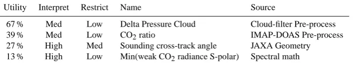
Utility measures the % contribution of a given feature to the overall filter performance. Interpret qualitatively measures how easily interpretable a researcher finds the feature. Restrict captures how restrictive to the resulting database a subfilter based on this feature would be.
Table 3. Features chosen by the genetic algorithm to reduce scatter over Sea (Glint mode).
Utility Interpret Restrict Name Source
67 % Med Low Delta Pressure Cloud Cloud-filter Pre-process 39 % Med Low CO2ratio IMAP-DOAS Pre-process
27 % High Med Sounding cross-track angle JAXA Geometry 13 % High Low Min(weak CO2radiance S-polar) Spectral math
higher complexity filters do not. MMS instability at the low-est transparencies is normal, as so few soundings are permit-ted through the filter that low-N statistics begin to dominate the scatter calculation. High transparency filters are seen to be extremely efficient by their slope, as it is an easier problem to eliminate the most egregious outliers initially.
Higher complexity is seen to reduce scatter at a fixed transparency due to its ability to more precisely fit the data with more parameters and access additional feature infor-mation; however, using complexities greater than four for land and three for sea are seen to have strongly diminish-ing returns. As we desire to maintain a high degree of in-terpretability of the sounding selector’s function, we prefer lower complexity. We choose to limit our complexity to two at this stage for the GOSAT example, for ease of graphing our results and interpretability in this example as well as sat-isfactory filter performance. However, one could in principle use a complexity four filter with only minor additional ef-fort. The future OCO-2 mission will likely employ a two-to-four complexity filter, as prescribed by its empirical trade-off curves. Note that at this stage, a complexity two filter might utilize many input features, but no more than two at any particular transparency. As an example, 60 % of the fil-ter’s transparency might be comprised of the pairing of sig-nal to noise ratio and co2_ratio, while the remainder of the curve might be constructed by the joining of co2_ratio and h2o_ratio. Three features would then be used, but only two at a time, thus complexity two. In the next section, we will impose the constraint of matching the total number of input features to the filter complexity to remove this detail.
4.2 Feature selection
4.2.1 Interpretability vs. utility
32 1
2
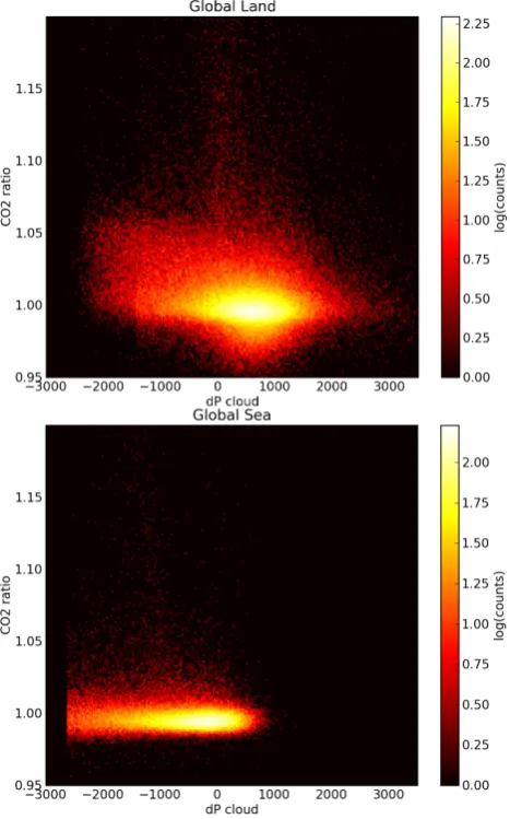
Figure 9. Land/sea sounding distributions for Delta Pressure Cloud (dPc) versus CO2 ratio. 3
Fig. 9. Land/sea sounding distributions for Delta Pressure Cloud
(dPc) versus CO2ratio.
are less desirable for this reason, as researchers often wish to observe the dependence of a measurable as a function of vari-ous angles or altitudes. Also problematic are features that are highly correlated withxCO2, as these might preclude regions
with true, large fluxes both positive and negative.
Comparing Tables 2 and 3 shows two features as highly significant (high utility, acceptable interpretability, and low restriction) in both land and sea cases: the CO2 ratio
(CO2r, unitless) and Delta Cloud Pressure (dPc, in hPa units). The first feature derives from the Iterative Maxi-mum A Posteriori Differential Optical Absorption Spec-troscopy (IMAP-DOAS) preprocessor in which CO2
con-centration estimates are independently derived for the strong and weak CO2bands within the radiance spectrum using a
non-scattering algorithm (Frankenberg et al., 2005). These estimates are not as robust as the GOSAT full physics re-trieval algorithm but orders of magnitude faster to compute. The unitless ratio of CO2 estimates from both the strong
33 1
Figure 10. Using only the two chosen features CO2 ratio (CO2r) and Delta Pressure Cloud 2
(dPc), the complexity=2 filters for land and sea are re-derived. Performance of the new 2-3
feature trade-off curves is similar to those using all-features, proving our feature selection was 4
successful. The small dip observed in the “Sea, All Features” curve near 5% transparency is 5
merely a sub-region where the cross-track sounding angle paired with CO2r was slightly more 6
efficient than dPc plus CO2r. 7
8 9
Fig. 10. Using only the two chosen features CO2 ratio (CO2r) and Delta Pressure Cloud (dPc), the complexity=2 filters for land and sea are re-derived. Performance of the new 2-feature trade-off curves is similar to those using all-features, proving our feature se-lection was successful. The small dip observed in the “Sea, All Fea-tures” curve near 5 % transparency is merely a subregion where the cross-track sounding angle paired with CO2r was slightly more ef-ficient than dPc plus CO2r.
1
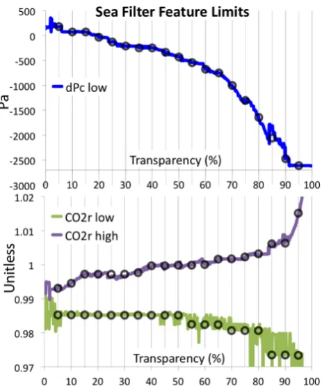
Figure 11. Land data sub-filter thresholds for dPc (top) and CO2r (bottom). Black circles 2
show monotonic, hand-smoothed final sub-filter values. 3
4
Fig. 11. Land data subfilter thresholds for dPc (top) and CO2r
35 1
Figure 12. Sea data sub-filter thresholds for dPc (top) and CO2r (bottom). Black circles show 2
monotonic, hand-smoothed final sub-filter values. Note that the high threshold for dPc was 3
not needed, as can be explained in Fig. 7, bottom. 4
5
Fig. 12. Sea data subfilter thresholds for dPc (top) and CO2r
(bot-tom). Black circles show monotonic, hand-smoothed final subfilter values. Note that the high threshold for dPc was not needed, as can be explained in Fig. 7, bottom.
and weak CO2 bands, CO2r, indicates enhanced scattering
within the atmosphere when different from 1.0. It is intu-itively satisfying that a spectral quality measure was selected as most useful. The second significant feature derives from the cloud filter preprocessor (Taylor et al., 2012), using the Oxygen A-band to derive surface pressure and goodness of fit assuming a Rayleigh-only atmosphere. The dPc is the dif-ference between the preprocessor’s quick-look surface pres-sure retrieved and the a priori surface prespres-sure as given by the European Centre for Medium-Range Weather Forecasts (ECMWF) model. This parameter is critical in the determi-nation of whether a sounding is too cloudy to process, as re-flective cloud tops will retrieve a substantially lower pressure than anticipated. Not only is this reasonable as a sounding selector input, but it speaks to the diffuse boundary between clear and cloudy sounding determination.
Other features we will not use that still yield insight are the geometric factors of solar zenith angle (shallow illumi-nation), cross-track angle (higher air mass), and standard de-viation of the altitude within the sounding (mountainous or highly sloped regions with ill-defined ray paths). All of these are highly interpretable and reasonable inputs for a sounding selector, lending evidence that the GA did indeed select ap-propriate features and that our Southern Hemisphere approx-imation/scatter reduction proxy for the truth is functioning.
36 1
2
Figure 13. The selector performance for transparency and scatter as a function of inclusive 3
warn levels. Permitting only warn level = 0 data (left of graph) is the most restrictive mode of 4
the filter, while accepting everything up through warn level 19 permits all the data to the 5
right. Note the deviation from original transparency as a function of warn level, caused by 6
enforcing monotonicity of filter thresholds, is very small. 7
8
Fig. 13. The selector performance for transparency and scatter as
a function of inclusive warn levels. Permitting only warn level=0 data (left of graph) is the most restrictive mode of the filter, while accepting everything up through warn level 19 permits all the data to the right. Note the deviation from original transparency as a func-tion of warn level, caused by enforcing monotonicity of filter thresh-olds, is very small.
Examining the distribution of CO2r versus dPc yields the decision boundary space fundamental to our future sound-ing selector (Fig. 9). We observe that the land has a much more dynamic CO2r range, while the sea shows strong bias in dPc relative to land. The cutoff used to determine cloudi-ness over the ocean is also observable for values less than
−2600 Pascals. 4.2.2 Targeted rerun
37 1
2
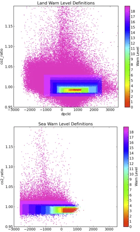
Figure 14. The definition of warn level as a function of CO2r and dPc. The optimal values of 3
CO2r ~ 0.99 and dPc ~ 800 hPa are different from 1.0 and 0.0 due to imperfect spectroscopy. 4
Fig. 14. The definition of warn level as a function of CO2r and dPc.
The optimal values of CO2r∼0.99 and dPc∼800 hPa are different from 1.0 and 0.0 due to imperfect spectroscopy.
4.3 Warn levels
To ensure we adequately represent the trade-off curves of Fig. 10 without having to compute a thousand filters per data point, we chose to sample the filters every 5 % transparency yielding 19 uniformly spaced dominant filters corresponding to the vertical graph lines of the figure. In Figs. 11 and 12 are shown the matching high and low thresholds for the subfilters for both CO2r and dPc as a function of transparency. The left-most region corresponding to low transparency show consid-erable noise, as the low number of data being accepted re-sults in low N statistics for the MMS. Noise in the right-most region of the graphs stems from some filter thresholds not be-ing actively used, as other thresholds dominate this high pass rate region such as for CO2r lower boundary for land or sea. Other more complex features such as near transparency 90 %
in the land case result from the interplay between thresh-olds. Left of this point, all four thresholds are cooperatively working to reduce scatter; however, to the right only the low threshold for dPc significantly contributes. There is nothing fundamentally inconsistent or problematic with such struc-ture from the point of view of the GA, as at each step a filter was generated that satisfied the scatter reduction and transparency requirements. However, we do require some additional properties for these threshold curves for a well-behaved sounding selector.
The uniformly sampled threshold values taken to imple-ment the warn levels are shown as black circles in Figs. 11 and 12. Note that while following the general trend of the GA solutions, they have been made monotone as a function of transparency. This will partially violate the precise relation-ship of warn level to transparency percentage, but will grant a very useful property that we will name selector stability: a se-lector is stable if for a given transparency all the data passed at lower transparencies is included. This prevents an indi-vidual sounding from being included at low transparencies, excluded at moderate transparencies, then included again at high transparencies. Such stuttering is admissible to the GA but makes defining a unique data grouping such as is required for the warn level impossible.
The final relationship of WL versus MMS and trans-parency can be found in Fig. 13. The desired transtrans-parency as a function of WL, initially defined as increments of 5 %, is closely approximated by our monotone filter. The relation-ship between dPc, CO2r, and WL for all global data (not merely the southern training data) is made clear in the de-cision boundary space of Fig. 14. Higher dimensional fil-ters (complexity>2) cannot be plotted so easily but are still quite useful and not significantly harder to derive by this same procedure.
Now that we have defined our warning levels, we can dis-card the ensemble of fixed filters and construct our sounding selector using only desired spatial coverage and the WL la-bels for each sounding. It should be stated that we make an assumption at this step that the thresholds we have defined in the Southern Hemisphere will also apply to the Northern Hemisphere.
4.4 Spatial coverage
38 1
Figure 15. Selector spatial coverage, color-coded by worst selected warn levels required for 2
each five degree latitude region for an example 20% transparency setting using actual 3
GOSAT data (full dataset). Note that cloudy regions near the equator and highly mixed terrain 4
such as shorelines are more problematic than large, flat regions. The unfilled regions in Africa 5
and the Arabian Desert are due to the omission of M gain data from this analysis. Warn Level 6
18 & 19 are never permitted to be selected, as they are too confounded to be useful for later 7
analysis. 8
9
Fig. 15. Selector spatial coverage, color-coded by worst selected warn levels required for each five degree latitude region for an example
20 % transparency setting using actual GOSAT data (full data set). Note that cloudy regions near the equator and highly mixed terrain such as shorelines are more problematic than large, flat regions. The unfilled regions in Africa and the Arabian Desert are due to the omission of M gain data from this analysis. Warn Level 18 & 19 are never permitted to be selected, as they are too confounded to be useful for later analysis.
39 1
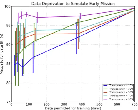
Figure 16. Using only two weeks of randomly selected training data, at least 85% and up to 2
96% of the optimal sounding selector was reconstructed. Note that the x-axis has been shifted 3
by a few days for each successive transparency for readability. The error bars represent the 4
stddev of the full data match % for the set of subwindows sampled. 5
Fig. 16. Using only two weeks of randomly selected training data,
at least 85 % and up to 96 % of the optimal sounding selector was reconstructed. Note that thexaxis has been shifted by a few days for each successive transparency for readability. The error bars rep-resent the stddev of the full data match % for the set of subwindows sampled.
terrain also show an increase in warn level. The large unfilled region in Africa and the Arabian desert is due to the omission of M-gain data from this analysis, not a failure of the sound-ing selector. We did not permit the selector to use any warn level 18 or 19 data, as it was judged of too poor quality to be desirable in any circumstance. Such soundings typically occur in the very challenging polar regions where low solar
angle, icy surfaces, and low-lying clouds conspire to prevent quality retrievals.
The confounding forces of cloud and complex terrain are well represented by the features we chose of CO2r and dPc. If we increased the complexity of the fixed filters admitted into our sounding selector construction above two, we could also use terrain roughness (filters mountainous regions) and overall spectral intensity (filters icy regions) as previously selected by the GA.
4.5 Required data volume, early mission
within error. We therefore conclude that a well-functioning sounding selector can be constructed after fully processing two weeks of data at the ACOS sampling rate of five sec-onds. As this sampling rate is sixty times slower than OCO-2, we should need only initially process 2 % of the incom-ing OCO-2 data for two weeks before the first-pass soundincom-ing selector can be produced. As we anticipate processing 6 %, there should be ample data within a few weeks for selector construction.
5 Summary
We have presented a procedure by which a sounding selec-tor may be generated using the output of a genetic algorithm (GA) that seeks to reduce the mean monthly scatter (MMS) in the Southern Hemisphere. The sounding features selected as most informative by the GA are hand-reviewed to optimize interpretability and reject undesired distortion of the data, making the method semi-autonomous. Any number of infor-mative features may be selected at this point; in the ACOS example, more than four was found to add negligible new in-formation. Adding features (higher complexity) reduces the simplicity of the sounding selector but can encompass addi-tional confounding forces and better fit the data. A uniform selection of fixed filters as a function of filter transparency (19 in the ACOS example) is then taken, and the thresh-olds of their subfilters are made monotone in transparency to preserve selector stability. This ensures that any data point permitted at a lower transparency will still be permitted at a higher transparency. The ensemble of uniformly sampled fixed filters is then used to define a warn level for each sound-ing equal to the number of filters that would reject it. Finally, we couple these warning levels to a spatial coverage routine that fills latitudinal bins with the lowest warn levels avail-able. The final product is a sounding selector with a tunable transparency that maximizes the likelihood of valid CO2
re-trievals from the selected soundings while guaranteeing spa-tial coverage. As an example point, given a 10 % throughput (transparency), the Land case’s mean monthly stdev (MMS) was reduced from 3.25 to 1.4 ppm, while the Sea case’s MMS was reduced from 3 to 1.2 ppm. However, 10 % is merely for example, and any requested percentage (rounded to the near-est 5 %) could be entered, yielding the list of bnear-est soundings to use.
This method is data-driven and agnostic to instrument. Any data set in which a goal function can be identified (i.e., the minimization of southern CO2scatter in our case) and
in-formative measurement features are present can be addressed in the same manner, even if the identities of the informative features are not known beforehand. Further, the execution of this method has been used to shed light onto the particular confounding forces acting upon the measurements by exam-ining the selected most informative features and examexam-ining their spatial and temporal distribution. This same technique
is now also implemented as a sounding quality estimation using post-retrieval features as well as those included here.
Acknowledgements. The research described in this paper was
carried out at the Jet Propulsion Laboratory, California Institute of Technology, under a contract with the National Aeronautics and Space Administration.
Edited by: H. Worden
References
Boesch, H., Backer, D., Connor, B., Crips, D., and Miller, C.: Global Characterization of CO2 Column Retrievals from
Shortwave-Infrared Satellite Observations of thet Orbiting Car-bon Observatory-2 Mission, Remote Sens., 3, 270–304, 2011. Conner, B., Boesch, H., Toon, G., Sen, B., Miller, C., and Crisp,
D.: Orbiting Carbon Observatory: Inverse method and prospec-tive error analysis, J. Geophys. Res.-Atmos., 113, D05305, doi:10.1029/2006JD008336, 2008.
Crisp, D., Atlas, R. M., Breon, F.-M., Brown, L.R., Burrows, J. P., Ciais, P., Connor, B. J., Doney, S. C., Fung, I. Y., Jacob, D. J., Miller, C. E., O’Brien, D., Pawson, S., Randerson, J. T., Rayner, P., Salawitch, R. J., Sander, S. P., Sen, B., Stephens, G. L., Tans, P. P., Toon, G. C., Wennberg, P. O., Wofsy, S. C., Yung, Y. L., Kuang, Z., Chudasama, B., Sprague, G., Weiss, B., Pollock, R., Kenyon, D., and Schroll, S.: The Orbiting Carbon Observatory (OCO) mission, Adv. Space Res., 34, 700–709, 2004.
Crisp, D., Fisher, B. M., O’Dell, C., Frankenberg, C., Basilio, R., Bösch, H., Brown, L. R., Castano, R., Connor, B., Deutscher, N. M., Eldering, A., Griffith, D., Gunson, M., Kuze, A., Man-drake, L., McDuffie, J., Messerschmidt, J., Miller, C. E., Morino, I., Natraj, V., Notholt, J., O’Brien, D. M., Oyafuso, F., Polonsky, I., Robinson, J., Salawitch, R., Sherlock, V., Smyth, M., Suto, H., Taylor, T. E., Thompson, D. R., Wennberg, P. O., Wunch, D., and Yung, Y. L.: The ACOS CO2retrieval algorithm – Part II:
Global XCO2data characterization, Atmos. Meas. Tech., 5, 687–
707, doi:10.5194/amt-5-687-2012, 2012.
Frankenberg, C., Platt, U., and Wagner, T.: Iterative maximum a posteriori (IMAP)-DOAS for retrieval of strongly absorbing trace gases: Model studies for CH4and CO2retrieval from near
infrared spectra of SCIAMACHY onboard ENVISAT, Atmos. Chem. Phys., 5, 9–22, doi:10.5194/acp-5-9-2005, 2005. Guerlet, S., Butz, A., Schepers, D., Basu, S., Hasekamp, O. P.,
Kuze, A., Yokota, T., Blavier, J.-F., Deutscher, N. M., Griffith, D., W., T., Hase, F., Kyro, E., Mornio, I., Sherlock, V., Suss-man, R., Galli, A., and Aben, I.: Impact of aerosol and thin cirrus on retrieving and validating XCO2 from GOSAT shortwave
in-frared measurements, J. Geophys. Res.-Atmos., 118, 4887–4905, doi:10.1002/jgrd.50332, 2013.
Guyon, I. and Elisseeff, A.: An Introduction to Variable and Feature Selection, J. Machine Learn. Res., 3, 1157–1182, 2003. Jin, Y. and Sendhoff, B.: Pareto-based multi-objective machine
the Orbiting Carbon Observatory, IEEE Trans. Geosci. Remote Sens., 49, 2426–2437, 2011.
O’Dell, C. W., Connor, B., Bösch, H., O’Brien, D., Frankenberg, C., Castano, R., Christi, M., Eldering, D., Fisher, B., Gunson, M., McDuffie, J., Miller, C. E., Natraj, V., Oyafuso, F., Polonsky, I., Smyth, M., Taylor, T., Toon, G. C., Wennberg, P. O., and Wunch, D.: The ACOS CO2retrieval algorithm – Part 1: Description and
validation against synthetic observations, Atmos. Meas. Tech., 5, 99–121, doi:10.5194/amt-5-99-2012, 2012.
Periaux, J. and Galan, M.: Genetic Algorithms in Engineering and Computer Science, John Wiley & Son Ltd, 1995.
Reuter, M., Bovensmann, H., Buchwitz, M., Burrows, J. P., Con-nor, B. J., Deutscher, N. M., Griffith, D. W. T., Heymann, J., Keppel-Aleks, G., Messerschmidt, J., Notholt, J., Petri, C., Robinson, J., Schneising, O., Sherlock, V., Velazco, V., Warneke, T., Wennberg, P. O., and Wunch, D.: Retrieval of atmospheric CO2 with enhanced accuracy and precision from
SCIA- MACHY: Validation with FTS measurements and com-parison with model results, J. Geophys. Res., 116, D04301, doi:10.1029/2010JD015047, 2011.
Taylor, T. E., O’Dell, C. W., O’Brien, D. M., Kikuchi, N., Yokota, T., Nakajima, T. Y., Ishida, H., Crisp, D., and Nakajima, T.: Com-parison of Cloud-Screening Methods Applied to GOSAT Near-Infrared Spectra, IEEE Trans. Geosci. Remote Sens., 50, 295– 309, 2012.
Wunch, D., Wennberg, P. O., Toon, G. C., Connor, B. J., Fisher, B., Osterman, G. B., Frankenberg, C., Mandrake, L., O’Dell, C., Ahonen, P., Biraud, S. C., Castano, R., Cressie, N., Crisp, D., Deutscher, N. M., Eldering, A., Fisher, M. L., Griffith, D. W. T., Gunson, M., Heikkinen, P., Keppel-Aleks, G., Kyrö, E., Lindenmaier, R., Macatangay, R., Mendonca, J., Messerschmidt, J., Miller, C. E., Morino, I., Notholt, J., Oyafuso, F. A., Ret-tinger, M., Robinson, J., Roehl, C. M., Salawitch, R. J., Sher-lock, V., Strong, K., Sussmann, R., Tanaka, T., Thompson, D. R., Uchino, O., Warneke, T., and Wofsy, S. C.: A method for eval-uating bias in global measurements of CO2total columns from
space, Atmos. Chem. Phys., 11, 12317–12337, doi:10.5194/acp-11-12317-2011, 2011.
Yokota, T., Oguma, H., Morino, I., and Inoue, G.: A nadir looking SWIR FTS to monitor CO2column density for Japanese GOSAT