Nonlinear Processes
in Geophysics
© European Geosciences Union 2003
Fractional Fourier approximations for potential gravity waves on
deep water
V. P. Lukomsky and I. S. Gandzha
Department of Theoretical Physics, Institute of Physics, Prospect Nauky 46, Kyiv 03028, Ukraine Received: 6 May 2003 – Revised: 15 August 2003 – Accepted: 2 September 2003
Abstract. In the framework of the canonical model of
hy-drodynamics, where fluid is assumed to be ideal and incom-pressible, waves are potential, two-dimensional, and sym-metric, the authors have recently reported the existence of a new type of gravity waves on deep water besides well studied Stokes waves (Lukomsky et al., 2002b). The distinctive fea-ture of these waves is that horizontal water velocities in the wave crests exceed the speed of the crests themselves. Such waves were found to describe irregular flows with stagnation point inside the flow domain and discontinuous streamlines near the wave crests.
In the present work, a new highly efficient method for computing steady potential gravity waves on deep water is proposed to examine the character of singularity of irregular flows in more detail. The method is based on the truncated fractional approximations for the velocity potential in terms of the basis functions 1/ 1 −exp(y0−y −ix)n, y0 be-ing a free parameter. The non-linear transformation of the horizontal scalex = χ −γsinχ , 0 < γ < 1, is addi-tionally applied to concentrate a numerical emphasis on the crest region of a wave for accelerating the convergence of the series. For lesser computational time, the advantage in accu-racy over ordinary Fourier expansions in terms of the basis functions exp n(y+ix)
was found to be from one to ten decimal orders for steep Stokes waves and up to one decimal digit for irregular flows. The data obtained supports the fol-lowing conjecture: irregular waves to all appearance repre-sent a family of sharp-crested waves like the limiting Stokes wave but of lesser amplitude.
1 Introduction
From old times the wave motion of the ocean bewitched and extremely attracted the attention of mankind. Up to now the problem of understanding specific features of water waves and their modelling represent a real challenge both from sci-entific and engineering points of view. Occurrence of
ex-Correspondence to: V. P. Lukomsky ([email protected])
tremely large and steep ocean breaking waves imposes a haz-ard to fishing boats, ships, and off-shore oil facilities. To understand physical mechanisms that give rise to extreme breaking waves and to model them correctly it is necessary to gain detailed knowledge of the form and dynamics of steep water waves.
The canonical problem about the propagation of surface waves on deep water (see Sect. 2) was the first essentially non-linear problem in hydrodynamics. Its analysis during almost two hundred years gave the origin to many fields of non-linear dynamics such as solitary waves, modulation in-stabilities, strange attractors, etc. Stokes (1847) was the first who considered surface waves of finite amplitude (Stokes waves). Small amplitude waves are sinusoidal. As the wave amplitude grows, the crests become steeper and sharper whilst the troughs flatten. Stokes (1880) conjectured that such waves must have a maximal amplitude (the limiting wave) and showed the flow in this wave to be singular at the crest forming a 120◦ corner (the Stokes corner flow). Much later, Grant (1973) suggested that this singularity, for a wave that has not attained the limiting form, is located above the wave crest and forms a stagnation point with streamlines meeting at right angles. Longuet-Higgins and Fox (1978) proved this numerically after extending Stokes flows analyti-cally outside the domain filled by fluid. The following ques-tion resulted: why the flow in the limiting Stokes wave has the 120◦singularity instead of the 90◦ one, as in any wave with lesser amplitude? Because of this Grant (1973) conjec-tured that a continuous approach to the limiting amplitude is possible only if the Stokes corner flow has several coalesc-ing scoalesc-ingularities. However, it has not yet clear where these multiple singularities arise from.
asymptotic expansions for waves close to the 120◦-cusped
wave (almost highest waves) and showed that these depen-dences oscillate infinitely as the limiting wave is approached. Nevertheless, strict numerical verification of such oscilla-tions seems to be a real challenge up to the present time, with only the first relative maximum and minimum having been thoroughly investigated (see, e.g. Longuet-Higgins and Tanaka, 1997).
Tanaka (1983) showed that gravity waves steeper than the wave with maximal total energy become unstable with re-spect to two-dimensional disturbances having the same pe-riod as an undisturbed wave (superharmonic instability). Jil-lians (1989) investigated the form of such instabilities and showed that they lead to wave overturning and breaking. The conjecture was made that wave breaking is a purely lo-cal phenomenon around the wave crest which, in the case of spilling breakers and more gently plunging breakers, oc-curs independently of the flow in the rest of a wave. Pro-ceeding with this idea Longuet-Higgins and Cleaver (1994) and Longuet-Higgins et al. (1994) suggested that superhar-monic instability results in the crests of almost highest Stokes waves to be unstable (crest instability). Longuet-Higgins and Tanaka (1997) strongly supported the conclusion that super-harmonic instabilities of Stokes waves are indeed crest insta-bilities. Finally, Longuet-Higgins and Dommermuth (1997) showed that crest instabilities lead (i) to wave overturning and breaking or (ii) to a smooth transition of a wave to a lower progressive wave having nearly the same total energy, followed by a return to a wave of almost the initial wave height. The latter fact generated a new question: what is the nature of such a transient phenomenon? A possible explana-tion would be found if superharmonic instability resulted in a bifurcation to a new solution, as usually takes place in non-linear dynamics. However, up to this time it was assumed that the Stokes solution is unique and free of bifurcations in keeping with the uniqueness argument of Garabedian (1965). The only bifurcation known to occur is the trivial one of a pure phase shift at the point of energy maximum (Tanaka, 1985).
The above results are all related to Stokes waves, for which the speed of fluid particles at the wave crests is smaller than the wave phase speed, equality being achieved for the limit-ing wave only. Thus, the traditional criterion for wave break-ing is that horizontal water velocities in the crest must ex-ceed the speed of the crest (Banner and Peregrine, 1993). Lukomsky et al. (2002a,b) have recently provided evidence (although numerical and not completely rigorous) for the ex-istence of a new family of two-dimensional irrotational sym-metric periodic gravity waves that satisfy the criterion of breaking. A stagnation point in the flow field of these waves is inside the flow domain, in contrast to the Stokes waves of the same wavelength. This makes streamlines exhibit discon-tinuity in the vicinity of the wave crests, with near-surface particles being jetted out from the flow. Because of this such waves and flows were called irregular (in contrast to regular Stokes flows).
To calculate irregular flows Lukomsky et al. (2002a,b)
used truncated Fourier expansions for the velocity poten-tial and the elevation of a free surface in the plane of spatial variables (a physical plane). Debiane and Kharif (see Gandzha et al., 2002) confirmed the existence of ir-regular waves using inverse plane Longuet-Higgins method (Longuet-Higgins, 1986), where the spatial coordinates are represented as Fourier series in velocity potential and stream function, the corresponding coefficients being evaluated by solving quadratic relations between them. Finally, Clam-ond (2003) also obtained irregular flows by applying his new renormalized cnoidal wave (RCW) approximation. In spite of this progress, irregular waves at present are only approxi-mate and not enough accurate numerical solutions. The fol-lowing question has to be answered then: what are the form and properties of irregular wave when its numerical error vanishes, that is, what real physical solutions do irregular waves approximate?
Ordinary Fourier expansions used by Lukomsky et al. (2002a) become not efficient enough for approximating ir-regular waves and even Stokes waves close to the limiting one due to slow descending of the Fourier coefficients. Thus, a more efficient method is necessary for these tasks. Up to now the most precise and efficient way for calculating the properties of two-dimensional surface waves is Tanaka’s method of the inverse plane (see Tanaka, 1983, 1986). The key idea of his method is to map the inverse plane into a unit circle by means of the Nekrasov transformation. Then boundary conditions are transformed to an integral equation, which is solved iteratively. The accuracy of obtained solu-tions is drastically improved by concentrating a numerical emphasis on the crest region using further transformation of variables. As a result, Tanaka’s method is the only one be-ing capable of evaluatbe-ing the second maximum of the phase speed and even further higher order extremums. In spite of all the advantages of Tanaka’s method and his program, where it is implemented, we are interested in improving the methods of the physical plane since they can be applied for calculating 3-D waves as well and can be generalized to the case of non-ideal and compressible fluid, in contrast to all the inverse plane methods.
Thus, the purpose of this paper is to present a new method in the physical plane for calculating two-dimensional poten-tial steady progressive surface waves on the fluid of infinite depth (see Sect. 3). The method is based on the fractional Fourier approximation for the velocity potential recently in-troduced by the authors (Gandzha et al., 2002; Lukomsky et al., 2002c) and the non-linear transformation of the hori-zontal scale for concentrating a numerical emphasis near the wave crest. The first term of such a fractional Fourier ap-proximation was independently derived by Clamond (2003) and was called a renormalized cnoidal wave approximation.
us-ing Tanaka’s method, proposed fractional Fourier approxi-mations have a potential to become almost as effective as the method of Tanaka. An additional set of stagnation points is found to exist above the crest area of Stokes waves sup-porting the conjecture of Grant (1973) that the 120◦ singu-larity of the limiting wave is formed of several coalescing 90◦singularities. In Sect. 4.2, the profiles of irregular waves are demonstrated to reveal the Gibbs phenomenon usually taking place when a discontinuous function or a continuous function with discontinuous derivatives are approximated by continuous truncated Fourier series. Moreover, even regu-lar Stokes waves very close to the Stokes corner flow are also demonstrated to exhibit the similar Gibbs phenomenon in accordance with the observation of Chandler and Graham (1993). The data presented resulted in the following assump-tion: irregular waves are very likely to approximate a family of sharp-crested waves like the limiting Stokes wave but of lesser amplitude. Concluding remarks are given in Sect. 5.
2 The canonical model
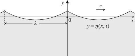
Consider the dynamics of steady potential two-dimensional periodic waves on the irrotational, inviscid, incompressible fluid with unknown free surface under the influence of grav-ity. Waves are assumed to propagate without changing their form from left to right along thex-axis with constant speed crelative to the motionless fluid at infinite depth (see Fig. 1). Gravity waves and related fluid flows are governed by the following set of equations
8θ θ+8yy=0, −∞< y < η(θ ); (1)
(c−8θ)2+82y+2η=c
2, y=η(θ ); (2) (c−8θ) ηθ+8y=0, y=η(θ ); (3)
8θ =0, 8y=0, y= −∞; (4)
whereθ=x−ctis the wave phase,8(θ, y)is the velocity potential (the velocity is equal to−→∇8),η(θ )is the elevation of the unknown free surface, andy is the upward vertical axis such thaty =0 is the still water level. Herein Eq. (1) is the Laplace equation in the flow domain, Eq. (2) is the dy-namical boundary condition (the Bernoulli equation,c2is the Bernoulli constant), Eq. (3) is the kinematic boundary con-dition (no fluid crosses the surface), Eq. (4) is the concon-dition that fluid is motionless at infinite depth. The dimensionless variables are chosen such that length and time are normal-ized by the wavenumberkand the frequency√gkof a linear wave, respectively,gbeing the acceleration due to gravity. In this case, the dimensionless wavelengthλ=2π.
When the total mass of the fluid is assumed to remain un-changed the wave mean level coincides with the still water level, that is,η=0, the overdash designating averaging over the wave period. The Bernoulli equation then results in the Levi-Civita relationq2=0, whereq2is the squared velocity at the free surface in the frame of reference moving together with the wave (the wave related frame of reference).
) , (x t y=η
y
x 0
λ
c
Fig. 1. The laboratory frame of reference.
Once the velocity potential and the wave phase speed are known, particle trajectories in the wave related frame of ref-erence (streamlines) are found from the following differential equations:
dθ
dt =8θ(θ, y)−c, dy
dt =8y(θ , y); (5) Each streamline is characterized by a constant value of a stream function ψ (θ, y)in the wave related frame of ref-erence. The velocity potential and the stream function 9(θ, y)=ψ (θ, y)+cyin the laboratory frame of reference are connected by means of the Cauchy-Riemann conditions: 8θ =9y; 8y= −9θ. (6)
This makes possible introducing the complex potentialW =
8+i9so that
8= −ic(R−R∗), 9=c(R+R∗), Rθ =iRy; (7)
whereR =iW∗/2c,∗is the complex conjugate. In terms of the complex functionR(θ, y), the dynamical and kinematic boundary conditions (2), (3) are as follows:
ic2 Rθ−Rθ∗
+2c2RθR∗θ+η=0, y=η(θ ); (8)
R(θ, η)+R∗(θ, η)−η=0. (9) Since the velocity potential and the stream function are de-fined to within an arbitrary constant the integration constant in Eq. (9) is included into the stream function to makeψ=0 at the free surface. Then9|y=η(θ ) =cη=0 and the stream function at infinite depth9|y=−∞=cη−I, where
I = 1
2π 2π
Z
0 dθ
η(θ )
Z
−∞
8θ(θ, y)dy=9 |y=η(θ )−9 |y=−∞.
is the wave impulse averaged over the period. The quantity K = I /c is the mass flux transferred by a wave over the period and is called the Stokes flow.
Eqs. (1), (8), (9), (4) of the canonical model the following quantities are to be found as the functions of the wave steep-nessA: the complex functionR(θ, y), the elevationη(θ )of the free surface, and the wave phase speedc.
3 The method for obtaining solutions
3.1 Fractional Fourier approximations
When working in the plane of spatial variables the solutions to the Laplace equation (1) in the flow domain are usually looked for as the following truncated Fourier series
R(θ, y)= N
X
n=0
ξnexp n(y+iθ )
. (10)
This approach was applied by the authors (Lukomsky et al., 2002a,b) for calculating steep gravity waves. Fourier ex-pansions (10), however, become ineffective for steep waves with sharpening crests close to the limiting wave due to slow descending of the Fourier coefficients. Because of this we proposed (Gandzha et al., 2002; Lukomsky et al., 2002c) a more effective set of functions to expand the velocity poten-tial on the basis of the following Euler formula (see Ham-ming, 1962)
∞
X
n=1
σnzn= ∞
X
n=1 ζn
1−z−1n, ζn=
n
X
n1=1
(−1)n1Cn1−1
n−1 σn1, (11) Cn1
n being the binomial coefficients. By choosingz(θ , y)=
exp(y−y0+iθ ); σn = ξnexp(ny0) the following one-parametric expansion for the velocity potential is obtained after truncating the series:
R(θ, y; y0)= N
X
n=0
ζn
1−exp(y0−y−iθ ) n
= N
X
n=0
αn
exp(−y0)−exp(−y−iθ )n ≡
N
X
n=0
αnTn(θ, y; y0), (12)
T (θ, y; y0)= exp(−y0)−exp(−y−iθ )
−1
, (13) where the normalized coefficientsαn =ζnexp(−ny0)were introduced to overcome infinite exponents at y0 → ∞; α0 ≡ ξ0. Approximation (12) shows a formal correspon-dence with Pad´e-type fractional approximates. Because of this we called expansion (12) a “fractional Fourier expan-sion”. It is singular in a countable number of isolated points y = y0,θ = 2π k, k ∈ Z, their location being determined by a free parameter y0. Singular points are to be located outside the flow domain for calculating potential waves. At y0 = ∞, fractional Fourier expansion (12) reduces to or-dinary Fourier expansion (10) withξn = (−1)nαn. Due to
Eq. (11), expansions (10) and (12) are equivalent atN = ∞
and the convergence of (12) follows from the convergence of Eq. (10). For finiteN andy0 ∼1, however, a fractional Fourier expansion converges much more rapidly than an or-dinary Fourier expansion. The reason is that a finite number of terms in Eq. (12) always corresponds to an infinite num-ber of terms in Eq. (10) that is especially important for waves with sharpening crests.
The zero constant term in expansions (12) and (10) is de-fined by the value of the stream function at infinite depth:
α0≡ξ0= 1
2c 9|y=−∞= 1
2 (η−K). (14)
Expansions (12), (10), and, in general, any function R(θ, y) = R(y+iθ ) all satisfy the Laplace equation (1) exactly. The latter fact was also used by Clamond (1999, 2003) (for finite and infinite depth, respectively) to introduce a renormalization principle that allows reconstructing the ve-locity potential in the whole domain once the veve-locity po-tential at the bottom (or any other level) is known. By ap-plying such renormalization to the first-order periodic solu-tion of KdV equasolu-tion Clamond (2003) obtained the velocity potential being exactly the same to the first term (N = 1) of expansion (12), which he called a renormalized cnoidal wave (RCW) approximation. There may be other possibili-ties to improve ordinary Fourier expansion (10) besides the proposed fractional expansion (12). However, one should ad-ditionally assure the convergence of series that makes con-structing such generalized expansions much more difficult.
One can see from the expansion of derivatives
Ry(θ, y; y0)= −iRθ = N+1
X
n=1
βnTn(θ, y; y0),
βn=nαn−(n−1)αn−1exp(−y0), (15) which follows directly from Eq. (12), that the boundary con-dition at infinite depth (Eq. 4) is also satisfied exactly.
Hereafter, only the symmetric waves are considered. In this case, the coefficientsαnandξnare real (in general, they
are complex numbers for nonsymmetric waves). After taking into account expansions (12) and (15) the boundary condi-tions (8), (9) at the free surface attain the following form:
2c2
N+1 X
n1=1
βn1Re(T n1)−
− N+1
X
n1=1 N+1 X
n2=1
βn1βn2Re(T
n1T∗n2)=η, y=η(θ ); (16)
2
N
X
n1=0
αn1Re(T
n1)−η=0, y =η(θ ). (17)
3.2 Nonlinear transformation of the horizontal scale To solve boundary conditions (16) and (17) one should assign an appropriate approximation to the unknown elevationy =
η(θ )of the free surface. In the plain of spatial variables, the Fourier series
η (θ )= ∞
X
n=−∞
ηn exp(inθ ), η−n=ηn, (18)
are often used. Note that the collocation method can be used instead but it is less efficient than expansion (18) (see Lukomsky et al., 2002b). The mean levelη =η0should be zero for exact solutions. For approximate solutions (when the series are truncated),η0becomes nonzero due to Levi-Civita relation not being held exactly and can be used to estimate the precision of approximate results.
Adequate description of sharpening profiles close to the limiting one requires taking into account excessively large number of modes due to extremely slow descending of the Fourier coefficients. This highly restricts practical applica-tion of Eq. (18). The following non-linear transformaapplica-tion of the horizontal scale originally suggested by Chen and Saffman (1980)
θ (χ; γ )=χ−γ sinχ , 0< γ <1, (19) allows overcoming this difficulty by stretching wave crests to a more rounded configuration. As a result, the Fourier series
η (χ; γ )= M
X
n=−M
ηn(γ ) exp(inχ ), η(γ )−n =η (γ )
n , (20)
in theχ-space with stretched crests are much more efficient (Lukomsky et al., 2002c). Due to nonlinear transformation (Eq. 19) any finite number M of the coefficients ηn(γ ) at
γ 6= 0 corresponds to infinite number of the coefficients ηn ≡ η(n0) in ordinary Fourier series (γ = 0), the
associ-ated relations being presented in Appendix A. Thus, the role of the parameterγ for the series (Eq. 18) in horizontal co-ordinateθis the same to the role of the parametery0for the series (Eq. 10) in vertical coordinatey.
3.3 Numerical procedure
By means of Eq. (20) the boundary conditions (16), (17) at the free surface are reduced to the following system of non-linear algebraic equations
Dn=c2dn−ηn(γ )=0, n=0, M; (21)
Kn=2 N
X
n1=1 αn1t
(n1) n −η
(γ )
n =0, n=1, N; (22)
where
dn=2 N+1 X
n1=1 βn1
t(n1)
n − N+1
X
n2=n1
βn2(2−δn1, n2) t (n1, n2) n
,
δn1, n2 is the Kronecker delta. The coefficients t (n1) n and
t(n1, n2)
n are the Fourier harmonics of the functions Re(Tn1)
and Re(Tn1T∗n2), respectively:
t(n1) n =
1 2π
2π
Z
0
ReTn1 θ (χ ), η(χ )
exp(−inχ )dχ ,
t(n1, n2)
n =
1 2π
2π
Z
0
Re Tn1T∗n2
exp(−inχ )dχ . (23)
They were calculated using the fast Fourier transform (FFT). The zero termα0and, therefore, the Stokes flowKare found from the kinematic equations (22) atn=0:
α0= 1 2η
(γ )
0 −
N
X
n1=1 αn1t
(n1)
0 , K=η−2α0. (24)
The truncation of Eqs. (21), (22) was chosen for the fol-lowing reasons. Since the set of kinematic equations (22) is linear over the coefficientsαn (n = 1, N), they can be
found in terms of the harmonicsηn(γ )without using
dynami-cal equations (21). To proceed in such a way, it is sufficient to take into account only the first N kinematic equations. Then the rest M+1 variables c, η(γ )0 , ηn(γ ) (n = 2, M)
are found from dynamical equations (21). The last un-known parameterη1(γ )is determined by the wave steepness A= η(0)−η(π )/2π as follows
η(γ )1 =π
2A−
[(M−1)/2]
X
n=1
η(γ )2n+1, (25) the square brackets designating the integer part. Since the wave steepness A is an integral characteristic, some wave properties may be missed when using it as a governing pa-rameter. Thus, we additionally use the first harmonicη1of the elevation in theθ-space (a spectral characteristic) as an independent variable instead of the wave steepness. In this case, the first harmonicη(γ )1 in theχ-space is expressed in terms ofη1and the rest of the harmonicsη(γ )n (n = 2, M)
by means of the expression (A1) atn=1 instead of Eq. (25). The set of Eqs. (21), (22) was solved by Newton’s method, the Jacoby matrix being given in Appendix B. Starting values for new calculations were taken from previous runs. For large enoughN andM, the Jacoby matrix was found to become badly conditioned. Because of this the program realization was implemented in arbitrary precision computer arithmetic. For instance, computations atN =150,M=2.5N demand 160-digit arithmetic that is ten times more accurate than the machine one. Note that such a run is equivalent in computer time to a run withN =250,M=4Nusing ordinary Fourier approximations and because of this takes approximately 4 times lesser computer memory.
for the elevation associated with this configuration, the num-berMshould be increased until the revision of solutions for greaterMbecomes less than chosen accuracy. Then the pre-cision to which boundary conditions (9) and (8) are satisfied defines the absolute errors connected with a truncation of the potential and elevation, respectively. Absolute errors of the dynamical and kinematic conditions divided by the constant terms contained in these equations, that is, the Bernoulli con-stantc2and the Stokes flowK, respectively, produce the cor-responding relative errors. The overall relative errorErmax of an approximate solution is agreed to be the maximal rel-ative error in boundary conditions (8) and (9) all over the wave period. To obtain a solution close to the exact one, one should gradually increase the numberN, choosing every time a proper value ofM, until overall desired precision is achieved. In a majority of calculations, it was sufficient to use the approximationM=2.5Nor lesser ones.
The numerical scheme proposed operates with two param-eters y0 and γ. Decreasingy0 from y0 = ∞ toy0 ∼ 1 accelerates the convergence of the fractional Fourier expan-sion (12) for the velocity potential, lesserNbeing necessary to retain the same accuracy. Increasingγ from γ = 0 to γ =1−ε, ε→0 accelerates the convergence of the expan-sion (20) for the elevation, lesserMbeing necessary to retain the same accuracy. These two processes, however, should be carried out simultaneously. Using the fractional Fourier expansion (12) without the transformation of the horizontal scale (19) was found to deteriorate the convergence of series (18) and, vice versa, using the transformation of the horizon-tal scale without the fractional Fourier expansion was found to deteriorate the convergence of expansion (10), with only slight overall benefit having been achieved. On the contrary, using the fractional Fourier expansion in combination with the nonlinear transformation of the horizontal scale proved to be highly efficient (see Sect. 4).
3.4 Physical quantities
Once the coefficientsαn,η(γ )n and the wave phase speedcare
found, a variety of wave characteristics can be calculated. The velocity potential, stream function, and the horizontal and vertical velocities of fluid particles are as follows:
8(θ, y)=2c
N
X
n=0
αnImTn(θ, y); (26)
9(θ, y)=2c
N
X
n=0
αnReTn(θ, y); (27)
8θ(θ, y)=2c N+1
X
n=1
βn ReTn(θ, y)
; (28)
8y(θ, y)=2c N+1
X
n=1
βn ImTn(θ, y); (29)
βn =nαn−(n−1)αn−1exp(−y0).
The horizontal and vertical accelerations of fluid particles are as follows:
d2θ
dt2 =8θ θ(8θ−c)+8yθ8y, d2y
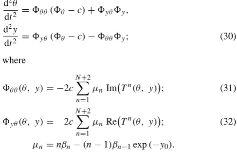
dt2 =8yθ(8θ−c)−8θ θ8y; (30) where
8θ θ(θ , y)= −2c N+2
X
n=1
µnIm Tn(θ, y); (31)
8yθ(θ , y)= 2c N+2
X
n=1
µnRe Tn(θ, y); (32)
µn=nβn−(n−1)βn−1exp(−y0).
The Stokes flowK, the wave impulseI, and the wave ki-netic energyEKin are as follows (see Cokelet, 1977, for ki-netic energy):
K=η0−2α0, I =Kc, EKin=cI /2; (33) α0 andη0 being determined from relations (14) and (A1), respectively.
The wave potential energyUis calculated as follows:
U= 1
2π 2π
Z
0 1 2 η
2(χ )dθ= 1 2 η
(γ ) 0
2
+ M
X
n1=1 η(γ )n1
2
− (34)
γ 2
η(γ )0 η(γ )1 + M
X
n1=1 η(γ )n1 η
(γ ) n1−1+η
(γ ) n1+1
.
4 Regular and irregular flows
4.1 Stokes flows
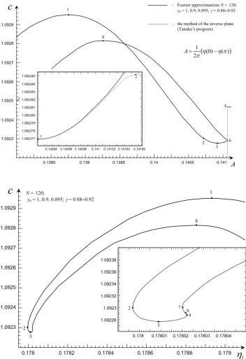
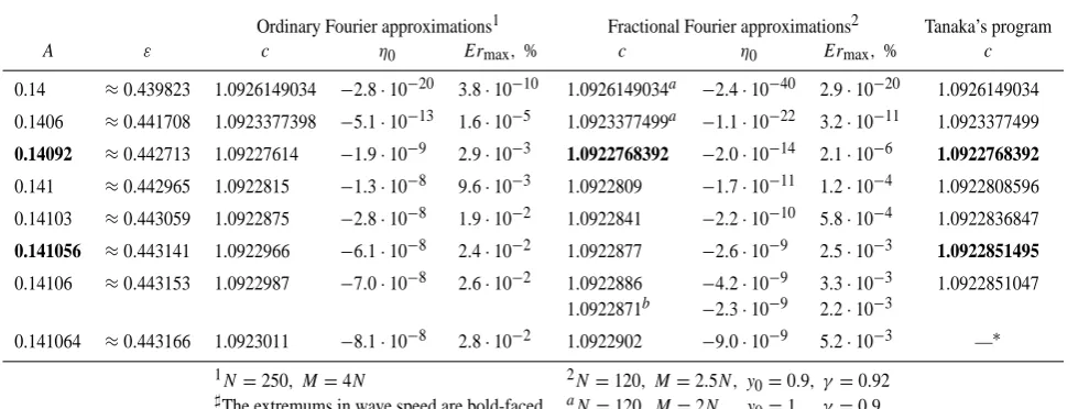
The dependencec(A)of the phase speed of almost highest Stokes waves on their steepness calculated using fractional Fourier approximations is shown in Fig. 2 by the branch 1-2-3-6. And the corresponding dependencec(η1)of the phase speed on the first harmonic of the elevation is presented in Fig. 3 by the branch 1-2-3-4-6. The corresponding points of extremums in phase speedc, the first harmonic η1, and steepnessAare presented in Table 1.
ten decimal orders forA = 0.14 (≈ 99.25% of the limit-ing steepness) to one decimal order forA = 0.141064 (al-most the limiting steepness). After taking into account that a run using fractional Fourier approximations withN =120, M =2.5N needs approximately 2.5 times lesser computer time and approximately 10 times lesser computer memory than a run using ordinary Fourier approximations withN =
250, M =4N, the advantage of fractional approximations becomes doubtless.
Nevertheless, the results presented for the values of steep-ness beyond the first minimum ofc(A =0.14092) are still less accurate than the ones obtained from Tanaka’s program, which are also included into Table 2 for comparison. This is also well seen from Fig. 2, where the second maximum ofc(A = 0.141056, the point 5) was obtained only using Tanaka’s program. The fractional Fourier approximation at y0 = 0.9 is sufficient to obtain the second maximum ofη1 (the point 4 in Fig. 3), but not sufficient to trace the second maximum ofc. The reason is that the valuey0=0.9 used is optimal for the steepness corresponding to the first minimum ofc, yet lessery0being necessary for greaterAto improve the precision of fractional Fourier approximations. However, using the present computer realization of the method the au-thors failed to accomplish this task due to unsatisfactory con-vergence of their numerical algorithm fory0 <0.9. If this problem could be resolved fractional Fourier approximations in the physical plane would have a potential to become al-most as effective as Tanaka’s method in the inverse plane.
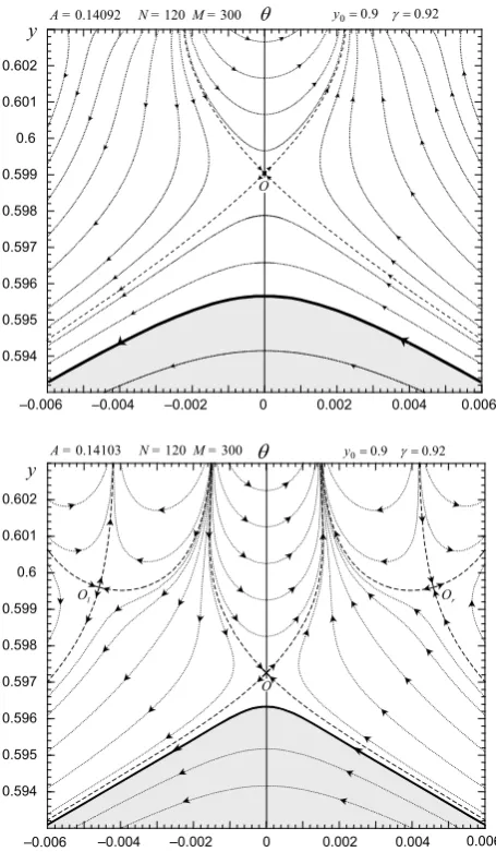
The flow field in Stokes waves is regular, that is, fluid par-ticles move slower than the wave itself all over the flow do-main. In the Stokes corner flow only, the fluid particle at the wave crest moves with velocity equal to the wave phase speed and, therefore, is motionless with respect to the wave. Because of this such points in the flow field are called the stagnation points. For all the Stokes waves other than the limiting one, a stagnation point is located outside the flow do-main, as was at first shown by Grant (1973). The examples of such regular flows mapped outside the domain filled by fluid are presented in Fig. 4 forA= 0.14092 andA=0.14103. The streamlines coming to/from the stagnation pointO(the separatrices) meet at right angles in accordance with the re-sults of Grant (1973) and Longuet-Higgins and Fox (1978). This is the general rule provided that the stagnation point and the wave crest do not merge (see Appendix C for de-tails). One can see from Fig. 4 that as the wave steepness is increased fromA=0.14092 toA=0.14103 the wave crest becomes sharper, the stagnation pointO and the crest ap-proaching each other. The downward and upward horn-like separatrices incoming to and outcoming from the stagnation pointO, respectively, become steeper and attain the vertical tangent closer to the vertical axis. In the limiting case, when the stagnation point and the wave crest completely merge, these two separatrices should come together and form a ver-tical line, where the upward and downward streamlines coin-cide. This provides a simple illustration how a vertical cut of the complex plane in the Stokes corner flow shown in Fig. D1 (see Appendix D) is formed.
It is not clear, however, how a 120◦corner at the crest of
the limiting Stokes wave is continuously formed from a 90◦
singularity that is inherent any flow at lesser amplitude. In view of this, Grant (1973) suggested that a 120◦ singular-ity should be formed from several coalescing singularities. The flow field shown in Fig. 4 atA =0.14103 provides an insight where these multiple singularities arise from. One can see that two additional symmetric 90◦stagnation points Or andOl exist above the wave crest at some distance from
the vertical axis. These lateral stagnation points also exist atA=0.14092 (and apparently at any lesser steepness) but are located outside the plot region in Fig. 4. Moreover, the pointsOr andOl are only the first ones in a whole set of
similar stagnation points located almost equidistantly in hor-izontal coordinate and having almost the same vertical po-sition at fixed A. As the wave steepness is increased, the pointsOr andOlmove towards the central stagnation point
O, the distance between all the stagnation points decreas-ing. Note that although the flow field in the domain filled by fluid and the position of the stagnation pointOin Fig. 4 are accurate enough, numerical accuracy sharply drops in the region, where the stagnation pointsOr andOl are located.
The flow field in this area has not been stabilized yet with respect to improving accuracy. As numerical accuracy is in-creased at fixedA, the lateral stagnation points all move to-wards the vertical axis, their vertical position remaining al-most unchanged. Therefore, they may finally settle down at the vertical axis above the stagnation pointO. Further inves-tigation is necessary to verify this assumption. Nevertheless, the existence of a set of additional stagnation points, which approach the central stagnation pointOas the steepness is in-creased, makes us expect that a 120◦singularity in the Stokes
corner flow is indeed formed from several (probably an infi-nite number of) coalescing 90◦ singularities supporting the conjecture of Grant (1973).
4.2 Irregular flows
Lukomsky et al. (2002b) have numerically revealed a new type of flows, where fluid particles move faster than the wave itself in the vicinity of the wave crest due to the stagnation point located inside the flow domain. Because of this such flows and waves were called irregular.
0.1385 0.139 0.1395 0.14 0.1405 0.141 1.0923
1.0924 1.0925 1.0926 1.0927 1.0928 1.0929
c
– the method of the inverse plane (Tanaka’s program)
– Fourier approximations N = 120; y0 = 1, 0.9, 0.895; γ= 0.88÷0.92
1
A Amax ( (0) ( ))
2
1 η ηπ
π −
=
A
2 3
6 8
0.14094 0.14096 0.14098 0.141 0.14102 0.14104 0.14106 1.092277
1.092278 1.092279 1.092280 1.092281 1.092282 1.092283 1.092284
3
5 1.092285
Fig. 2. The dependence of the phase speedcof steep surface waves on their steepnessA.
0.178 0.1782 0.1784 0.1786 0.1788 0.179
1.0923 1.0924 1.0925 1.0926 1.0927 1.0928 1.0929
c
N = 120;y0 = 1, 0.9, 0.895; γ= 0.88÷0.92
1
1
η
38
2
0.178 0.17801 0.17802 0.17803 0.17804
1.09228 1.0923 1.09232 1.09234 1.09236 1.09238
2
3
4 7
6
Fig. 3. The dependence of the phase speedcof steep surface waves on the first harmonicη1of their profile.
Fig. 3 (the curve 4-6-7). As the limiting point 6 is passed in this way, the wave steepnessAcan again be used as a govern-ing parameter to obtain the whole irregular branch 6-8 shown in Figs. 2 and 3.
While moving along the irregular branch away from the limiting point 6 the accuracy of approximate solutions at fixedN andMdrops since the stagnation point settles down deeper into the flow domain. Because of this the branches corresponding to irregular flows in Figs. 2, 3 have not yet sta-bilized with respect to increasing the truncation numbersN
Table 1. The points of extremums in phase speedc, steepnessA(ε = π A), and the first harmonicη1of the profile for Stokes waves
(N=120, M=2.5N, y0=0.9, γ=0.92)
point extremum A ε c η1
the first max ofη1 0.1351 0.424429 1.0909437483 0.1799822
1 the first max ofc 0.13875 0.435896 1.0929513818 0.1789318
2 the first min ofη1 0.14072 0.442085 1.0923021558 0.1779969
3 the first min ofc 0.14092 0.442713 1.0922768392 0.1780099
4 the second max ofη1 ≈0.141055 0.443137 ≈1.092288 0.1780222
5∗ the second max ofc 0.141056 0.443141 1.0922851495
6 max ofA(the limiting value) ≈0.141064 0.443166 ≈1.09229 0.1780216
∗
Results from Tanaka’s program
Table 2. The wave speedcand the mean water levelη0for steep Stokes waves depending on their steepnessA(ε =π A)]. The maximal
relative errorsErmaxof corresponding approximate solutions demonstrate great advantage of fractional approximations over ordinary Fourier
approximations
Ordinary Fourier approximations1 Fractional Fourier approximations2 Tanaka’s program
A ε c η0 Ermax, % c η0 Ermax,% c
0.14 ≈0.439823 1.0926149034 −2.8·10−20 3.8·10−10 1.0926149034a −2.4·10−40 2.9·10−20 1.0926149034
0.1406 ≈0.441708 1.0923377398 −5.1·10−13 1.6·10−5 1.0923377499a −1.1·10−22 3.2·10−11 1.0923377499
0.14092 ≈0.442713 1.09227614 −1.9·10−9 2.9·10−3 1.0922768392 −2.0·10−14 2.1·10−6 1.0922768392
0.141 ≈0.442965 1.0922815 −1.3·10−8 9.6·10−3 1.0922809 −1.7·10−11 1.2·10−4 1.0922808596
0.14103 ≈0.443059 1.0922875 −2.8·10−8 1.9·10−2 1.0922841 −2.2·10−10 5.8·10−4 1.0922836847
0.141056 ≈0.443141 1.0922966 −6.1·10−8 2.4·10−2 1.0922877 −2.6·10−9 2.5·10−3 1.0922851495
0.14106 ≈0.443153 1.0922987 −7.0·10−8 2.6·10−2 1.0922886 −4.2·10−9 3.3·10−3 1.0922851047 1.0922871b −2.3·10−9 2.2·10−3
0.141064 ≈0.443166 1.0923011 −8.1·10−8 2.8·10−2 1.0922902 −9.0·10−9 5.2·10−3 —∗
1N=250, M=4N 2N=120, M=2.5N, y
0=0.9, γ=0.92 ]The extremums in wave speed are bold-faced aN=120, M=2N, y
0=1, γ =0.9 bN=150, M=2.5N, y
0=0.9, γ=0.92
∗The maximum steepness in Tanaka’s program isA≈0.1410635
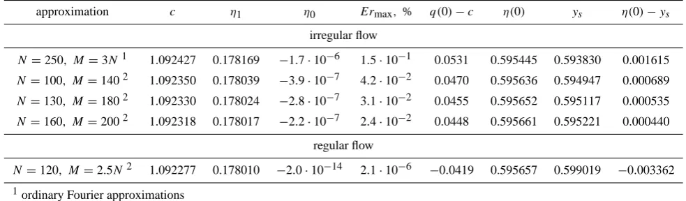
the turning point than is obtained at present since the regular branch is expected to have an infinite number of extremums incandη1in the case of being evaluated exactly. Because of this it is also not clear now whether there is a bifurcation to the irregular branch from the Stokes branch. Much more accurate calculations and, therefore, further improvement of the method are necessary to clarify these points and to stabi-lize the position of the irregular branch.
Thus, our main concern is that irregular flow is an ap-proximate solution, whose accuracy is not sufficient enough to make definite conclusions even when using fractional ap-proximations. Nevertheless, some progress was achieved.
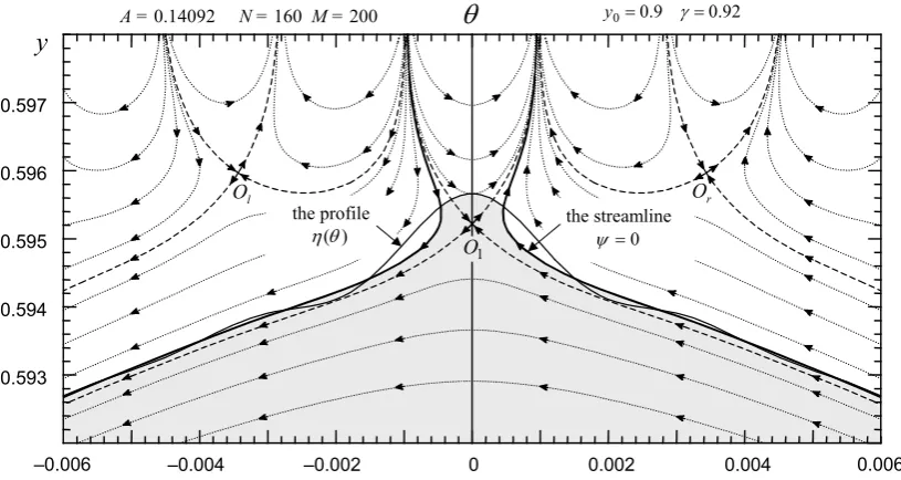
Consider the example of the irregular flow calculated us-ing fractional Fourier approximations atA = 0.14092 and shown in Fig. 5, with the streamlines mapped outside the
Table 3. The parameters of the irregular flow atA=0.14092 for different approximations:cis the wave phase speed;η1is the first harmonic
of the elevation;η0is the mean water level (it should be zero for exact solutions);Ermaxis the maximal relative error of an approximate
solution;q(0)−cis the velocity at the crest in the wave related frame of reference;η(0)is the height of the crest above the still water level; ys is the vertical position of the stagnation point;η(0)−ys is the distance of the stagnation point from the wave crest. The same parameters of the regular flow atA=0.14092 are also included for comparison∗
approximation c η1 η0 Ermax, % q(0)−c η(0) ys η(0)−ys
irregular flow
N=250, M=3N1 1.092427 0.178169 −1.7·10−6 1.5·10−1 0.0531 0.595445 0.593830 0.001615
N=100, M=1402 1.092350 0.178039 −3.9·10−7 4.2·10−2 0.0470 0.595636 0.594947 0.000689
N=130, M=1802 1.092330 0.178024 −2.8·10−7 3.1·10−2 0.0455 0.595652 0.595117 0.000535
N=160, M=2002 1.092318 0.178017 −2.2·10−7 2.4·10−2 0.0448 0.595661 0.595221 0.000440
regular flow
N=120, M=2.5N2 1.092277 0.178010 −2.0·10−14 2.1·10−6 −0.0419 0.595657 0.599019 −0.003362
1ordinary Fourier approximations
2fractional Fourier approximationsy
0=0.9, γ=0.92
∗
for the Stokes corner flow,c≈1.0923,η(0)=c2/2≈0.59656,ys=η(0)
dependence. Because of this the streamlineψ=0 describes a free surface near the wave crest more adequately than the wave profileη(θ ).
What is the nature of this inaccuracy? It is seen from Fig. 5 that the profile of the irregular flow oscillates while ap-proaching the wave crest, where a prominent peak (an over-shoot) forms. This highly resembles the Gibbs phenomenon when (i) a discontinuous function or (ii) a continuous func-tion with discontinuous derivatives (a weak discontinuity) are approximated by a truncated set of continuous functions (see, e.g. Arfken and Weber, 1995). In both cases, the Gibbs phe-nomenon is an excellent indicator of a singularity. Thus, ir-regular waves correspond to singular solutions of the equa-tions of motion.
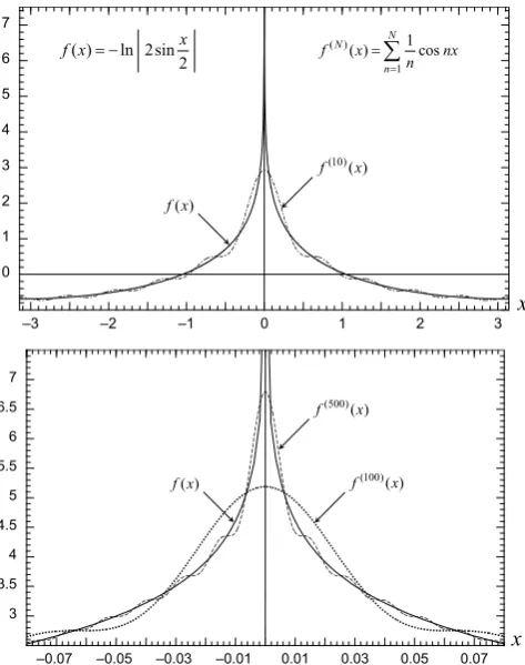
The example corresponding to the case (i) is given in Appendix E, where truncated Fourier series of a function with infinite discontinuity are demonstrated to exhibit typical Gibbs oscillations and an overshoot that moves to infinity as accuracy is improved (see Fig. E1). In contrast to this exam-ple, however, the overshoot in the profile of irregular waves has an almost fixed vertical position and shrinks both in ver-tical and horizontal scales as numerical accuracy is improved when proceeding from the ordinary to fractional Fourier ap-proximations, as one can see from Fig. 6. The same situation is observed for regular Stokes waves very close to the Stokes corner flow having a sharp 120◦ corner at the crest (a dis-continuous first derivative) that corresponds to the case (ii) of weak discontinuity. Such waves also exhibit Gibbs os-cillations when being approximated numerically, as was re-vealed by Chandler and Graham (1993) from the analysis of Nekrasov’s integral equation. The similar example obtained using fractional and ordinary Fourier expansions is presented in Fig. 7 for the Stokes wave atA=0.14106 (≈99.9975% of the limiting steepnessA≈ 0.1410635). The Gibbs
phe-nomenon is distinctly observed and the overshoot shrinks both in vertical and horizontal scales with increasing the ac-curacy of approximations in the same way as the overshoot of the irregular wave presented in Fig. 6. In the case of the limit-ing Stokes wave, the overshoot is absent in the exact solution that has a sharp 120◦ corner at the crest, that is, it shrinks completely. Thus, the conclusion can be made that the over-shoot in the profile of irregular waves should to all appear-ance also shrink into a single point when increasing accuracy further. What would the wave profile look like then?
To answer this question let us analyse how the param-eters of an approximate irregular flow at fixed steepness A =0.14092 depend on improving numerical accuracy us-ing Table 3. The distanceη(0)−ys between the wave crest
and the stagnation point becomes approximately four times as small when using more accurate fractional approxima-tions instead of ordinary Fourier approximaapproxima-tions, the hori-zontal and vertical dimensions of the overshoot both becom-ing approximately five times as small. This correlates with decreasing the maximal relative errorErmaxof the solutions approximately by a factor of six. The particle velocity at the crestq(0)−cin the wave related frame of reference also de-creases but less rapidly than the relative errorErmax of the corresponding solutions. On the contrary, the wave height η(0)quickly stabilizes with increasing accuracy and seems not to tend to the height of the Stokes corner flow.
pro-–0.004 –0.002 0 0.002 0.004 0.006 0.594
0.595 0.596 0.597 0.598 0.599 0.6 0.601 0.602
–0.006
y θ y0=0.9 γ=0.92
O A = 0.14092 N = 120 M = 300
r O l
O
–0.004 –0.002 0 0.002 0.004 0.594
0.595 0.596 0.597 0.598 0.599 0.6 0.601 0.602
–0.006 0.006
y θ y0=0.9 γ=0.92
O A = 0.14103 N = 120 M =300
Fig. 4. The regular flow in the crest region of almost highest Stokes waves at two different values of the wave steepness, in the wave related frame of reference, the streamlines mapped outside the do-main filled by fluid being presented as well.
file coinciding with the streamlineψ = 0 all over the free surface. The Stokes theorem about a 120◦corner flow (see
Appendix D) is generally valid for corner flow independently of the wave amplitude. Therefore, irregular waves to all ap-pearance turn out to approximate a family of sharp-crested waves with 120◦corner at the crest like the limiting Stokes wave but of lesser steepness. Sharp-crested corner flows and regular Stokes flows both tend to the Stokes corner flow as the wave steepness is increased. Moreover, the additional stagnation pointsOl andOr in Fig. 5 approach to the
cen-tral stagnation pointO1as numerical accuracy is improved. Therefore, the stagnation point at the crest of sharp-crested waves should to all appearance also be formed from several coalescing singularities similar to the limiting Stokes wave.
Although irregular flows with stagnation point inside the flow domain are only approximate numerical solutions, they can be used for simulating the process of wave breaking. One
can see from Fig. 5 that the particles from the near-surface layer of the irregular flow are accelerated to velocities greater than the wave phase speed when approaching the crest. As a result, they form the upward jet emanating from the front face of the wave. The acceleration of particles at the base of the jet ranges from 2.5gatθ=0.001 to 6gat the wave crest. Such large accelerations of the water rising up the front of the wave into the jet are in fact known to occur in breaking waves (see Banner and Peregrine, 1993), where the typical maxima in accelerations obtained from detailed unsteady numerical computations were reported to be around 5g. The following subsequent unsteady evolution of irregular flow is expected. The particles with velocities greater than the wave speed will all be jetted out away from the fluid and the crest will break if their is no external influx into the flow domain from the left downward jet. After finishing this non-stationary process the flow will become regular and of lesser steepness. This re-sembles the recurrence phenomenon observed by Longuet-Higgins and Dommermuth (1997) when computing unsteady non-linear development of the crest instabilities of almost highest Stokes waves resulting in a smooth transition to a periodic wave of lower amplitude. The appearance of irregu-lar flows in their numerical scheme may be a reason for this phenomenon.
5 Conclusions
Fractional Fourier approximations for the velocity potential in combination with non-linear transformation of the hori-zontal scale, which concentrates a numerical emphasis on the crest region, turned out to be much more efficient than ordinary Fourier approximations when computing both steep regular and irregular flows. Nevertheless, further improve-ment of the numerical algorithm is necessary to achieve the accuracy of Tanaka’s method when calculating almost lim-iting Stokes waves and to attain the final understanding of irregular flows. One of the possible ways is to use the fol-lowing multi-term fractional expansion with several different parametersyk:
R(θ, y; {yk})= K
X
k=0 Nk X
n=0
α(k)n
exp(−yk)−exp(−y−iθ )n
.
r
O
l
O
–0.004 –0.002 0 0.002 0.004
0.593 0.594 0.595 0.596 0.597
–0.006 0.006
y
θ
92 . 0 9 . 0
0= γ=
y
A = 0.14092 N = 160 M = 200
the profile ) (θ η
1
O
the streamline 0
= ψ
Fig. 5. The profile and streamlines of the irregular flow near the wave crest, in the wave related frame of reference, the streamlines mapped outside the domain filled by fluid being presented as well.
–0.02 –0.015 –0.01 –0.005 0 0.005 0.01 0.015 0.02 0.025 0.585
0.59 0.595
–0.025
η
θ
– the Stokes corner flow
the irregular wave – the irregular wave
y0 = 0.9, γ= 0.92
y0 = ∞, γ= 0, N = 250, M = 3N
the Stokes wave
A = 0.14092 (ε≈ 0.442713)
N = 160, M = 200
Fig. 6. The behavior of the overshoot (the Gibbs phenomenon) in the profile of the irregular wave when improving numerical accuracy due to proceeding from the ordinary to fractional Fourier approximations. The profile of the Stokes wave of the same steepness is also included for comparison.
–0.015 –0.01 –0.005 0 0.005 0.01 0.015
0.59 0.592 0.594 0.596
η
θ
– the Stokes corner flow – N = 250, M = 4N, y0 = ∞, γ= 0
A = 0.14106 (ε≈ 0.443153) – N = 150, M = 2.5N,
y0 = 0.9, γ= 0.92
terms of the fractional expansion). In the case of finite depth h, the fractional Fourier expansion will be as follows:
R(θ, y; y0)= N
X
n=0
αn(+)
exp(−y0)−exp(−y−h−iθ ) n −
αn(−)
exp(−y0)−exp(y+h+iθ )n
.
Finally, fractional expansions may also be generalized to the case of 3-D waves and non-ideal fluid.
Fractional approximations allowed us to gain more de-tailed knowledge about the properties of irregular flows. Ir-regular waves were proved to correspond to singular solu-tions of the equasolu-tions of motion. Because of this their ex-istence does not contradict to the uniqueness theorem of Garabedian (1965) since it deals with regular continuous so-lutions only. The profiles of exact soso-lutions (sharp-crested waves) corresponding to irregular waves seem to have a sharp 120◦ corner at the crest (a discontinuous first derivative) like the limiting Stokes wave but of lesser amplitude. Such solutions are also known to occur in the physics of shock waves, where they are called the surfaces of weak discon-tinuity (see Landau and Lifshitz, 1995). Further analysis, however, should be carried out to make a final conclusion. One of the possible ways is to investigate how an approxi-mate irregular flow depends on taking into account surface tension and to make a comparison with new limiting forms for gravity-capillary waves recently obtained by Debiane and Kharif (1996).
To conclude note that the formation of jets from irregular progressive waves resembles the occurence of vertical jets with sharp-pointed tips from standing gravity waves forced beyond the maximum height, as has recently been reported by Longuet-Higgins (2001).
Acknowledgements. We are grateful to Prof. M. Tanaka for being so kind to place at our disposal his program for calculating Stokes waves. We express thanks and appreciation to Professors D.H. Pere-grine, C. Kharif, V.I. Shrira, and Dr. D. Clamond for many valuable advices and fruitful discussions. The research of I. Gandzha has been supported by INTAS Fellowship YSF 2001/2-114.
Appendix A The relations between the Fourier coeffi-cients in theθ- andχ-spaces
Taking into account nonlinear transformation (19) the coeffi-cients in Fourier series (18) and (20) are connected as follows η0=η0(γ )−γ η
(γ ) 1 ,
ηn=
1 n
M
X
n1=1
n1η(γ )n1 Jn−n1(nγ )−Jn+n1(nγ )
, (A1)
n=1, ∞;Jn(z)being the Bessel function of the first kind.
Appendix B The Jacoby matrix
The Jacoby matrix is composed of the coefficients at the in-finitesimal variationsδc, δη0(γ ), δηn(γ )1 (n1 = 2, M), δαn1 (n1=1, N) of the unknown variables in the following vari-ations of equvari-ations (21) and (22):
δDn = N
X
n1=1 αn, n22
1δαn1 + M
X
n1=0 αn, n21
1δη (γ )
n1 +2c dnδc;
δKn = N
X
n1=1 αn, n12
1δαn1 + M
X
n1=0 αn, n11
1δη (γ ) n1 ;
where αn, n11
1 =α 11 n−n1 +α
11 n+n1, α
11
n,0=α11n ;
αn, n121 =2t(n1)
n ; α11n =2 N+1
X
n1=1 βn1t
(n1) n −δn,0;
αn, n21 1 =α
21 n−n1 +α
21 n+n1, α
21 n,0=α
21 n ;
α21n =2c2
N+1 X
n1=1 βn1
n1 tn(n1)−t(n1 +1)
n e
−y0−
N+1 X
n2=n1
(2−δn1, n2) βn2 (n1+n2) t (n1, n2)
n −
n1tn(n1+1, n2)e −y0−n
2tn(n1, n2+1)e −y0
−δn,0;
αn, n22
1 =2n1c 2t(n1)
n −t(n1 +1)
n e
−y0−
2
N+1 X
n2=1 βn2 t
(n1, n2) n −t
(n1+1, n2)
n e
−y0.
Note that the variationδη(γ )1 should be expressed in terms of the rest variations δηn(γ ),n = 2, M using expression (25)
if the governing parameter is the steepnessAor the relation (A1) atn=1 if the governing parameter is the first harmonic η1of the elevation in theθ-space.
Appendix C The stagnation point
The point in the flow field, where fluid particles are mo-tionless in the wave related frame of reference, is called the stagnation point. For symmetric regular/irregular flows, the stagnation point is located above/below the wave crest out-side/inside the flow domain on the axis θ = 0. Then its vertical positionysis determined as follows
8θ(0, ys)=c. (C1)
To find the velocity field8θ(θ, y),8y(θ, y)in the
in-finitesimal vicinityθ = ˜θ (θ˜ → 0),y = ys + ˜y (y˜ → 0)
Fig. D1. A local 120◦corner flow, the cut of the complex plane being dashed.
Tn(θ, y)around the stagnation point as follows
T (θ, y)=T (ys+ ˜y+iθ )˜ =T (ys)+T0(ys)(y˜+iθ )˜ ;
Tn(θ, y)=Tn(ys)+nT0(ys)Tn−1(ys)(y˜+iθ ).˜ (C2)
Then, after taking into account condition (C1), the Eqs. (5) for particle trajectories attain the following form in the vicin-ity of the stagnation point:
dθ˜ dt =ay,˜
dy˜
dt =a
˜
θ; a=2c
∞
X
n=1
nβnT0(ys)Tn−1(ys).
Therefore, the equations for the streamlines areθ˜ = ± ˜y.
Actually, this is a direct consequence of the fact that any so-lution to the Laplace equation (1) should depend not on the variables (θ,y) separately but on their combinationy+iθ.
Thus, the streamlines meet at right angles (90◦) at the stag-nation point. This fact is valid for any flow provided that the stagnation point and the wave crest do not merge. Other-wise,ys =η(0);θ˜andx˜are not independent variables, and
linearization (C2) is not valid. In this case, the streamlines turn out to meet at 120◦angle (see Appendix D), as was at first shown by Stokes (1880).
Appendix D The Stokes theorem
Stokes rigourously showed that the only possible local crest singularity of a steady wave is a corner of 120◦. Hereafter we emphasize that Stokes theorem is generally valid for a wave of any amplitude, not only for the limiting wave.
Choose the origin of the wave related frame with upward vertical axisy and left-to-right horizontal axisθat the wave crest. Let φ (θ, y) be the velocity potential in the wave related frame. Choose the stream functionψ (θ, y) to be
–3 –2 –1 0 1 2 3
0 1 2 3 4 5 6 7
x
2 sin 2 ln )
(x x
f =−
∑
=
=N
n
N nx
n x f
1 )
( () 1cos
) (x f
) (
) 10 ( x
f
–0.07 –0.05 –0.03 –0.01 0.01 0.03 0.05 0.07 3
3.5 4 4.5 5 5.5 6 6.5 7
x )
(x
f f(100)(x) ) (
) 500 ( x
f
Fig. E1. The truncated Fourier series of the discontinuous function. The Gibbs phenomenon.
zero at the free surface. In terms of the complex coordi-nate z = θ +iy = rexp(iϕ) and the complex potential w(z)=φ+iψ, the Bernoulli equation (2) is as follows:
dw dz 2
+2 Imz=0. (D1)
The complex potential for a flow including a sharp corner with stagnation point is described by the following function: w(z)=Azn= |A|rnexp(inϕ+iϕA), (D2)
where −3π/2 < ϕ < π/2,ϕ = π/2 being the cut of the complex plane. Substitution of (D2) into the Bernoulli equa-tion (D1) yieldsn = 3/2. Note that (D2) is only locally valid being only the first term in an expansion about the cor-ner. Further terms include the powers of irrational order as was established by Grant (1973) and Norman (1974).
The condition thatψ =0 at the corner slopes yields (the corner angle is 2α):
sin3
2 α −
π 2
+ ϕA
=0⇒ 3
2 α −
π 2
+
ϕA=π,
sin3 2 −α−
π 2
+ϕA
=0⇒ 3
2 −α− π 2
+ϕA=0.
Thereforeα = π/3, ϕA = 5π/4, and the corner angle is
wave known to exhibit such a corner flow is the Stokes wave of limiting amplitude. It seems that irregular waves reveal a family of similar corner flows with amplitudes less than that of the limiting Stokes wave. The Stokes corner flow seems to be formed due to merging the stagnation points of regular and irregular flows at limiting amplitude.
Appendix E The Gibbs phenomenon
Consider the following 2π-periodic function f (x)= −ln
2 sin x 2
(E1)
with infinite discontinuity atx = 2π k, k ∈ Z. This func-tion constitutes a part of the kernel of Nekrasov’s integral equation (see Chandler and Graham, 1993). The truncated Fourier series of the functionf (x)have the following form (see Arfken and Weber, 1995):
f(N )(x)= N
X
n=1 1
ncos(nx), f (x)=Nlim→∞f
(N )(x). (E2)
In this case, the discontinuous functionf (x)is approximated by the continuous functions f(N )(x). One can see from Fig. E1 that instead of infinite discontinuities, the functions f(N )(x) have rounded peaks (overshoots) with symmetric oscillatory tails that descend as the distance from the point of discontinuity increases. This is the well known Gibbs phenomenon, which always takes place when approximating discontinuous functions by the truncated Fourier series (see Arfken and Weber, 1995). As the numberN is increased, the functionsf(N )(x)approximate the functionf (x)more precisely. The peak moves upwards and the oscillatory tails move closer to the point of discontinuity, their amplitude and period decreasing. Nevertheless, the height of the peak (the vertical distance between the point x = 0 and the point, where the oscillatory tail initiates) remains almost constant with increasingN. Because of this the truncated Fourier se-ries representation remains unreliable in the vicinity of a dis-continuity even for high enoughN.
References
Arfken, G. B. and Weber, H. J.: Mathematical Methods for Physi-cists, Academic Press, London, 1995.
Banner, M. L. and Peregrine, D. H.: Wave breaking in deep water, Ann. Rev. Fluid Mech., 25, 373–397, 1993.
Chandler, G. A. and Graham, I. G.: The computation of water waves modelled by Nekrasov’s equation, SIAM J. Numer. Anal., 30, 1041–1065, 1993.
Chen, B. and Saffman, P. G.: Numerical evidence for the existence of new types of gravity waves of permanent form on deep water, Stud. Appl. Math., 62, 1–21, 1980.
Clamond, D.: Steady finite-amplitude waves on a horizontal seabed of arbitrary depth, J. Fluid Mech., 398, 45–60, 1999.
Clamond, D.: Cnoidal type surface wave in deep water, J. Fluid Mech., 489, 101–120, 2003.
Cokelet, E. D.: Steep gravity waves in water of arbitrary uniform depth, Philos. Trans. Roy. Soc. London, 286, 183–221, 1977. Debiane, M. and Kharif, C.: A new limiting form for steady
pe-riodic gravity waves with surface tension on deep water, Phys. Fluids, 8, 2780–2782, 1996.
Gandzha, I. S., Lukomsky, V. P., Lukomsky, D. V., Debiane, M., and Kharif, C.: Numerical evidence for the existence of a new type of steady gravity waves on deep water, in: Geophys. Res. Abstracts, vol. 4, pp. A–01 347, EGS 27th General Assembly, Nice, France, 2002.
Gandzha, I. S., Lukomsky, V. P., Tsekhmister, Y. V., and Chalyi, A. V.: Comparison of ordinary and singular Fourier approxima-tions for steep gravity and gravity-capillary waves on deep water, in Geophys. Res. Abstracts, vol. 5, pp. A–12 192, EGS-AGU-EUG Joint Assembly, Nice, France, 2003.
Garabedian, P. R.: Surface waves of finite depth, J. Analyse Math., 14, 161, 1965.
Grant, M. A.: The singularity at the crest of a finite amplitude pro-gressive Stokes wave, J. Fluid Mech., 59, 257–262, 1973. Hamming, R. W.: Numercal Methods, Mc Graw-Hill, New York –
San Francisco – Toronto – London, 1962.
Jillians, W. J.: The superharmonic instability of Stokes waves in deep water, J. Fluid Mech., 204, 563–579, 1989.
Landau, L. D. and Lifshitz, E. M.: Fluid Mechanics (Course of Theoretical Physics, Vol. 6), Pergamon Press, New York, 1995. Longuet-Higgins, M. S.: Integral properties of periodic gravity
waves of finite amplitude, Proc. Roy. Soc. London, A342, 157– 174, 1975.
Longuet-Higgins, M. S.: Bifurcation and instability in gravity waves, Proc. Roy. Soc. London, A403, 167–187, 1986.
Longuet-Higgins, M. S.: Asymptotic forms for jets from standing waves, J. Fluid Mech., 447, 287–297, 2001.
Longuet-Higgins, M. S. and Cleaver, R. P.: Crest instabilities of gravity waves. Part 1. The almost highest wave, J. Fluid Mech., 258, 115–129, 1994.
Longuet-Higgins, M. S. and Dommermuth, D. G.: Crest instabili-ties of gravity waves. Part 3. Nonlinear development and break-ing, J. Fluid Mech., 336, 33–50, 1997.
Longuet-Higgins, M. S. and Fox, M. J. H.: Theory of the almost highest wave: the inner solution, J. Fluid Mech., 80, 721–741, 1977.
Longuet-Higgins, M. S. and Fox, M. J. H.: Theory of the almost highest wave. Part 2. Matching and analytic extension, J. Fluid Mech., 85, 769–786, 1978.
Longuet-Higgins, M. S. and Tanaka, M.: On the crest instabilities of steep surface waves, J. Fluid Mech., 336, 51–68, 1997. Longuet-Higgins, M. S., Cleaver, R. P., and Fox, M. J. H.: Crest
instabilities of gravity waves. Part 2. Matching and asymptotic analysis, J. Fluid Mech., 259, 333–344, 1994.
Lukomsky, V. P., Gandzha, I. S., and Lukomsky, D. V.: Computa-tional analysis of the almost-highest waves on deep water, Comp. Phys. Comm., 147, 548–551, 2002a.
Lukomsky, V. P., Gandzha, I. S., and Lukomsky, D. V.: Steep sharp-crested gravity waves on deep water, Phys. Rev. Lett., 89, 164 502, 2002b.
Lukomsky, V. P., Gandzha, I. S., Lukomsky, D. V., Tsekhmister, Y. V., and Chalyi, A. V.: Computational analysis of periodic gravity waves on a free water surface in the vicinity of limit-ing steepness, in Bull. Amer. Phys. Soc., vol. 45(5), pp. 34–35, Conference on Computational Physics, San Diego, California, 2002c.
Stokes waves, J. Fluid Mech., 66, 261–265, 1974.
Stokes, G. G.: On the theory of oscillatory waves, Camb. Phil. Soc. Trans., 8, 441–455, 1847.
Stokes, G. G.: Considerations relative to the greatest height of oscil-latory waves which can be propagated whithout change of form, Math. Phys. Papers, 1, 225–228, 1880.
Tanaka, M.: The stability of steep gravity waves, J. Phys. Soc. Japan, 52, 3047–3055, 1983.
Tanaka, M.: The stability of steep gravity waves. Part 2, J. Fluid Mech., 156, 281–289, 1985.