www.nonlin-processes-geophys.net/19/439/2012/ doi:10.5194/npg-19-439-2012
© Author(s) 2012. CC Attribution 3.0 License.
Nonlinear Processes
in Geophysics
Evolutionary modeling-based approach for model errors correction
S. Q. Wan1,2, W. P. He3, L. Wang4, W. Jiang5, and W. Zhang6
1Yangzhou Meteorological Office, Yangzhou, China
2Department of Physics, Yangzhou University, Yangzhou, China
3National Climate Center, China Meteorological Administration, Beijing, China 4School of Computer Science, Beijing Institute of Technology, Beijing, China 5Jiangsu Meteorological Bauru, Nanjing, China
6Department of Atmospheric Sciences, Lanzhou University, Lanzhou, China Correspondence to: W. P. He (wenping [email protected])
Received: 3 December 2011 – Revised: 20 July 2012 – Accepted: 24 July 2012 – Published: 14 August 2012
Abstract. The inverse problem of using the information of
historical data to estimate model errors is one of the science frontier research topics. In this study, we investigate such a problem using the classic Lorenz (1963) equation as a pre-diction model and the Lorenz equation with a periodic evo-lutionary function as an accurate representation of reality to generate “observational data.”
On the basis of the intelligent features of evolutionary modeling (EM), including self-organization, self-adaptive and self-learning, the dynamic information contained in the historical data can be identified and extracted by computer automatically. Thereby, a new approach is proposed to esti-mate model errors based on EM in the present paper. Nu-merical tests demonstrate the ability of the new approach to correct model structural errors. In fact, it can actualize the combination of the statistics and dynamics to certain extent.
1 Introduction
Monthly, seasonal, annual and inter-annual climatic predic-tions became the next targets of the frontier research of at-mospheric sciences since the successful implementation of short-term weather forecasts. However, with the discovery of chaos, it is well known that the climate system is a com-plex nonlinear system, and climate prediction is a great chal-lenge to researchers. Moreover, inherent defects of statistical methods and dynamical methods result in significant uncer-tainties of their applications in climate prediction. Statistical methods are mainly used to search prediction clues from his-torical observational data, based on the hishis-torical behavior
and statistical regularities of the climate system. The results of statistical model are sometimes satisfactory, but such sta-tistical regularities and the prediction models derived from such statistical methods are often unstable due to the effects of nonlinearity of the climate system (Gu, 1958).
The prediction problem based on dynamical methods can be regarded as a problem of initial value of differential equa-tions. It implies that it is necessary to ensure sufficiently pre-cise initial values and boundary conditions as well as the ac-curacy of the prediction model in order to obtain a reliable prediction. In fact, these conditions cannot be satisfied com-pletely. Despite the continuous improvement and optimiza-tion of numerical model and data assimilaoptimiza-tion systems, it is difficult to improve the time limit of weather forecasts be-yond two weeks (Lorenz, 1965, 1969) due to the complexity of the atmospheric motion. Therefore, it is crucial to develop alternative ways to improve the capability of the climate pre-diction model (Schubert, 1985; Vannitsem and Toth, 2002; Chou, 2003a, b; Li and Ding, 2011).
Chou (2007) argued that past daily weather changes, espe-cially the recent evolutionary status of the atmosphere, con-tain the information of numerical model errors. It should be used to correct the model errors. Some related mathematical and numerical issues in the geophysical fluid dynamics and climate dynamics have been discussed (Li and Wang, 2008). These methods have shown to be useful techniques for cli-mate prediction in numerical experiments and applications. It is an evidence of the effectiveness of the dynamics-statistics approach.
In fact, the idea of the correction of the model errors is old. Many studies provided some objective methods of estimat-ing model errors, but their use for improvestimat-ing model perfor-mance, is comparatively small. Examples are given by Schu-bert (1985), Klinker and Sardeshmukh (1992). D’Andrea and Vautard (2000) proposed a methodology for the correction of systematic errors in a simplified atmospheric general cir-culation model, and confirmed that this improvement actu-ally stems from the flow dependence of the model error. Such flow dependence was found in the Euro-Atlantic sec-tor, while similar attempts to establish this relation in other sectors of the globe failed. Vannitsem and Toth (2002) inves-tigated the short-term dynamics of model errors by means of numerical analysis of the Lorenz (1984) low-order atmo-spheric system, and found that the short-term mean square error evolution is mainly characterized by an initial quadratic or linear behavior, depending on the dynamical properties of the model error source terms. Also, there are studies of the impact of model errors associated with parameter errors. Duan and Zhang (2010) investigated the effect of initial er-rors and model parameter erer-rors on a significant “spring pre-dictability barrier” (SPB) for El Ni˜no events. They inferred that initial errors, rather than model parameter errors, may be the dominant source of uncertainties that cause a signifi-cant SPB for El Ni˜no events. Mu el al. (2010) suggested that conditional nonlinear optimal perturbation approach (CNOP) can be applied to estimate model parameter errors for El Ni˜no events, but did not consider other kinds of model errors at present. Despite this, it is expected that CNOP will play an important role in the studies of atmospheric and oceanic sci-ences.
However, most of the works mentioned above remain in the theoretical stage, and many issues need to be addressed for their application in weather forecasts (Chou et al., 2007). For example, traditional methods for solving inverse prob-lems of differential equations face one essential problem of ill-posed characteristic, such as the instability of approxi-mate solutions. The models describing the complex cliapproxi-mate system can only approximately describe the major dynamic processes of atmospheric motion. Therefore, not all the de-tails are described in these prediction models. In fact, climate change can be viewed as a long-range evolutionary process with self-adaptation. So, it is unnecessary to describe all the characteristics of the problem in detail, and all it requires is
a solution in accordance with the evolutionary laws of the nature.
In the case that only limited information is known on a dynamic system, a possibility is to replace human intelli-gence with computational intelliintelli-gence in some steps of the traditional modeling, including the development of assump-tions, the construction and the calculation of the model. This is the idea of so-called evolutionary modeling (EM; Cao et al., 2000). Evolutionary computation is a mathematical modeling approach based on the evolutionary laws of nature (Back et al., 1997; Cao et al., 2000). In EM, simple cod-ing techniques can be used to represent a variety of com-plex mathematical structures. The approximate solutions of inverse problem can be automatically searched by computer programs. This step is iterated for some number of genera-tions until the termination criterion of the run has been satis-fied. The characteristics of evolutionary algorithms are self-organizing, self-adaptive and self-learning. Natural selection, namely survival of the fittest, and evolution strategies provide many conveniences and advantages for solving inverse prob-lems of complex differential equations.
In the present work, the problem of how to use combina-tion of the dynamics and statistics to correct model errors has been studied. On the basis of the EM method, a new approach is proposed to correct model errors. Using the new approach, dynamic information of model errors can be extracted from historical observational data. The results of numerical exper-iments based on the Lorenz (1963) model have been prelim-inarily validated in terms of their ability to correct model er-rors. It must be noted that the model error studied here mainly refers to the dynamic structural error in a prediction model.
2 Algorithm of EM
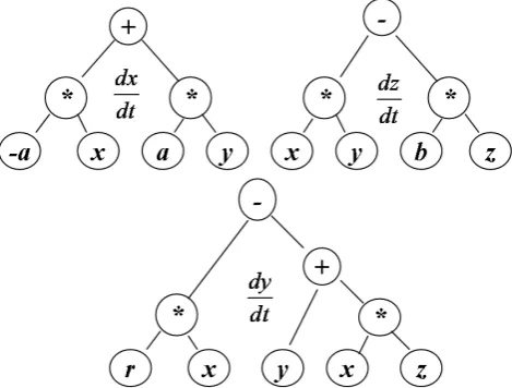
Fig. 1. Hierarchical structure diagram of binary tree of the Lorenz model.
termination criterion of the run has been satisfied. The com-plexity of a function can be controlled by setting the depths of the layers of a binary tree. The detailed algorithm of EM can be found in Cao et al. (2000). As an example, the classic three-dimensional Lorenz (1963) model can be written as the form:
dx
dt =ax+ay=Lx(x, y) dy
dt =rx−(y+xz)=Ly(x, y, z) dz
dt =xy−bz=Lz(x, y, z).
(1)
Here, the three parameters,a, r andb, are positive, and are called the Prandtl number, the Rayleigh number and a phys-ical proportion related to convective scale, respectively. In the present study, the three parameter values are 10.0, 28.0 and 8/3, respectively. When r >24.74, the Lorenz system exhibits chaotic behavior. The binary tree form of the Lorenz model is shown in Fig. 1.
In evolutionary algorithms, an individual mathematical model structure corresponds to a unique binary tree (Fig. 1). Three popular methods can be used to implement evolution-ary computation, namely, genetic algorithm (GA), gene ex-pression programming (GEP; Ferreira, 2001), and genetic programming (GP; Saiedian, 1997). The GP and GEP meth-ods will be selected to implement EM program in the present study.
3 Correction scheme for model errors
Numerical prediction models are the dynamic equations con-structed according to the basic laws of atmospheric and cli-mate motion as currently understood. Undoubtedly, these models use simplified and approximate equations. It can only describe main features of atmospheric motion. In fact, the
problem is that the disturbance terms have to be overlooked, or certain important dynamic elements are not included due to the limitation of the existing knowledge. One of the current measures for correcting errors is a post-processing strategy for model prediction results, i.e. statistically correct on the prediction results. However, the omission of dynamic char-acteristics of the model error affects the quality of the results of the statistical correction.
3.1 Description of the inverse problem
An inverse problem is a general framework that is used to convert observed measurements into information about a physical object or system that we are interested in. For ex-ample, if we have measurements of the Earth’s gravity field, then we might ask the question: “given the data that we have available, what can we say about the density distribution of the Earth in that area?” The solution to this problem (i.e. the density distribution that best matches the data) is use-ful because it generally tells us something about a physi-cal parameter that we cannot directly observe (Keller, 1976; http://en.wikipedia.org/wiki/Inverse problem).
In contrast, with a forward problem, an inverse problem of differential equations is based on existing results to de-duce the cause of the results. In other words, on the basis of the solution or partial solution of one differential equation, the unknown components of the equation can be deduced. In terms of differential equations, Leverentiev and his col-leagues argued that the inverse problem can be defined as follows: an inverse problem for a partial differential equation is any problem involving the determination of the coefficients or right-hand side of a partial differential equation on the ba-sis of certain functionals of the solution of the equation (Lev-erentiev et al., 2003). Without loss of generality, the general form of differential equations can be written as
L·u(x, y, t )=f (x, y, t ), (x, y)∈, t∈(0,∞). (2) Here,L is the differential operator, and u(x, y, t )is the solution of the differential equation. The functionf (x, y, t ) is the right-hand side source term of the equation. When L is unknown, this is called an inverse problem of opera-tor identification; furthermore, when the right-hand source termf (x, y, t ) is unknown, this is called a source-term verse problem. The ill-posedness and nonlinearity of an in-verse problem make the related theories and solutions more complex and difficult than those of a forward problem.
dx
dt =Lx(x, y)3Ex(x, y, z) dy
dt =Ly(x, y, z)3Ey(x, y, z) dz
dt =Lz(x, y, z)3Ez(x, y, z).
(3)
Here, E(x, y, z) is the potential unknown error term, which is a composite function, such as trigonometric, ex-ponential and power functions. The symbol “3” represents connecting nodes. Generally, the symbol can only be basic arithmetic operators, such as “+,−,×,÷”. IfL(x, y, z) is the main dynamic structure of the function, “3” can be deter-mined. In this case, the symbol “3” usually is “+”. Even for a simple dynamic equation, such as Eq. (1), it is difficult to determine the specific mathematical expression ofE(x, y, z) using traditional methods. On the basis of the definition of the inverse problem, determining the error term E(x, y, z) in Eq. (3) is a classic inverse problem, namely, solving the source term on the right-hand side.
The limitation of those traditional methods is that model structure must be determined in advance, and then model pa-rameters can be estimated. However, it generally depends on personal experience to construct model structure. It is a com-plicated problem, especially when the data space takes on the form of hyper-surfaces with parameters and multi-variables.
3.2 Error correction scheme of evolutionary
algorithm-based prediction model
The main steps for correcting prediction model error terms through historical data are as follows: an approximate predic-tion model and an accurate predicpredic-tion model are constructed, respectively. The solutions of the approximate model are re-garded as the prediction results of a specific system, and the solutions of the accurate model are regarded as “obser-vational data”. Subsequently, the EM algorithm is used to automatically search for the error term. During modeling, a large ensemble of mathematical model structures is ran-domly formed by means of the search in the basic function library using the evolution program. Simultaneously, the pa-rameters of the individual model structures will be continu-ously estimated and optimized by the parameter optimization module. According to certain criteria, poor individual model structures will be eliminated, and good model structures will be retained, which can be continuously used to EM of the next generation. Finally, several mathematical models with relatively minimal errors will be obtained.
Firstly, in Eq. (3), for example, the function L(x, y, z) must be unchanged in the EM. Then, the function will be expressed as the binary tree hierarchy (Fig. 1), which can be represented in a certain program code, and then can be placed into the evolutionary process. Obviously, obtaining the ex-pression of the error functionE(x, y, z)is an inverse problem
that solves the right-hand side of the differential equation. Here,L(x, y, z)is the approximate model, and the correction scheme of the prediction equation is as follows.
1. Constructing Gene(L), the binary tree of the main func-tionL(x, y, z).
2. Specifying randomly the node symbols and the con-stants contained in the error terms E(x, y, z), and the nodes include {+,−,×,÷,sin,cos,ln,exp}in the present study. The populations Pop with a certain size will be generated randomly.
3. Forming several binary tree structures Genei(E)of the error functions using the evolutionary algorithm GP and GEP. Meanwhile, Genei(E) will concurrently evolve with the main binary tree Gene(L) by applying evo-lutionary operations, including selection, hybridization and mutation. By controlling the depths of the binary tree layers of Genei(E), several complex-controllable composite binary trees (i.e. the revised function) can be obtained.
4. Computing and evaluating the adaptive values of these composite binary trees in combination with “ob-servational data”. Retaining the superior individuals Genei(E)in the generation, and then these superior in-dividuals will be used as EM of the next generation. 5. Repeating the above procedures until a new function
body meets the predetermined conditions (i.e. the ter-mination condition).
3.3 Numerical experiments
In order to test the performance of the error correction scheme presented in this study, it is necessary to generate “observational data”. To deal with this issue, a classic three-dimensional Lorenz model is regarded as an inaccurate pre-diction equationL(x, y, z). The Lorenz model with an error termEx=5 sin(sin(x))is regarded as an accurate prediction equation, and connecting node3=“+00, as follows:
∧ =“+00
Ex(x, y, z, t )=5 sin(sin(t )) Ey(x, y, z, t )=0
Ez(x, y, z, t )=0.
Thus, Eq. (3) can be written as
dx
dt =Lx(x, y)+5 sin(sin(t )) dy
dt =Ly(x, y, z) dz
dt =Lz(x, y, z).
(4)
- 2 0 - 1 5 - 1 0 - 5
0
5
1 0 1 5 2 0
0 1 0 0 2 0 0 3 0 0 4 0 0 5 0 0 6 0 0 7 0 0 8 0 0
5
1 0 1 5 2 0 2 5 3 0 3 5 4 0 4 5 5 0
X 0
X
X
Z 0
Z
Z
n
(a )
(b )
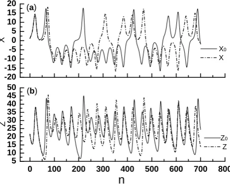
Fig. 2. The “observed value” (x0, z0) and the corresponding predic-tion data (x, z) of the predicpredic-tion model, where the sample size is 700. (a) Variablexin the Lorenz model; and (b) variablezin the Lorenz model.
700 integral steps of Eq. (4) are regarded as “observed data” (solid line in Fig. 2). The corresponding prediction data can be generated by the classic Lorenz model (Eq. 1), and the so-lution of the approximation model has been shown in Fig. 2 (dash line). Comparing the prediction data with the obser-vational data, it is clear that there is some small difference between the prediction data and the observational data when the integral time is less than about 180 steps. Thereafter, the differences gradually become larger, and even the phases of evolution of the prediction data and the observational data are sometimes in opposition.
In accordance with the correction scheme, the GP and GEP are used in the modeling approach. The details of the related parameters are already listed in Table 1, and a relative error function is used as the fitness function,
fitness(f (x))= 100.0
N P
i=1
(xi−xi0)2
. (5)
Equation (5) is called the evaluation function, which is a quantitative indicator of the quality of model, and also pro-vides the termination condition of the EM program. Here, xi is the “observational data”, andxi0 is the solutions of the
revised model by EM. It is the most crucial element of the evolutionary algorithm for the problem to be solved. The selection of the fitness function has a significant impact on the convergence speed and results of the evolutionary algo-rithm. The evaluation function (Eq. 5) is comparatively con-sistent with the law of evolution, the “survival of the fittest”. It retains a suitable adaptive range and can create a state space that can be addressed by the evolutionary algorithm. A suitable evaluation function can improve the convergence
- 2 0 - 1 0
0
1 0 2 0
1 0 2 0 3 0 4 0 5 0
- 2 0 - 1 0
0
1 0 2 0
0 1 0 0 2 0 0 3 0 0 4 0 0 5 0 0 6 0 0 7 0 0 8 0 0
1 0 2 0 3 0 4 0 5 0
X
X 0
X f o r E x ( 1 ) X f o r E x ( 2 ) X f o r E x ( 3 )
Z
Z 0
Z f o r E x ( 1 ) Z f o r E x ( 2 ) Z f o r E x ( 3 )
(a )
(b )
(c )
(d )
X
X 0
X f o r E x ( 4 ) X f o r E x ( 5 ) X f o r E x ( 6 )
Z
n
Z0
Z f o r E x ( 4 ) Z f o r E x ( 5 ) Z f o r E x ( 6 )
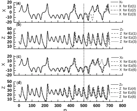
Fig. 3. Error correction based on the first componentLx(x, y)using EM. (a) and (b) are the fitting and prediction data of the corrected models using the error functionE(x1),Ex(2)andEx(3), respectively. (c) and (d) are the same as (a) and (b), but forEx(4), Ex(5), Ex(6), respectively.
velocity of the evolutionary algorithm and avoid excessively rapid or slow evolution of populations. Thus, it can ensure to obtain several reliable solutions with high quality. A few prediction equations have been listed in Table 2 obtained by the error correction scheme.
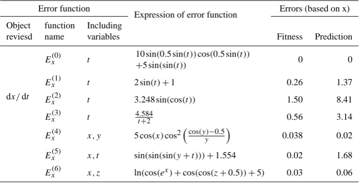
Generally, it is difficult to have the knowledge on the forms and positions of the error terms. The error corrections have been implemented for the three functions Lx(x, y), Ly(x, y, z),Lz(x, y, z), respectively. Based on the results of the EM, seven representative error functions are shown in Ta-ble 2 for the error corrections on the first functionLx(x, y)in the Lorenz model (Eq. 1). The error functionE(x0) obtained by EM is identical to the real error term because the func-tion Ex(0) can be transformed into the original error func-tion. Indeed, it is no doubt that the probability for obtain-ing an identical error function is very low in climate models based on the existing technology. The reason is that the vari-ables and physical mechanisms of the atmospheric motion are more complicated than those of the current example. The other six error functions can be divided into two categories. The first three error functions only contain time variablet, and the style of these functions is similar to that of the real error function. In contrast, there are more than one variable contained in the other three error functions. It is easy to find that most of these error functions obtained by EM are similar to the given error termEx, namely, trigonometric functions are the main form in these error functions.
Table 1. Parameters in the EM procedure.
Setting GP GEP
Population size 100 100
Generation 100–1000 500–1000
Selection method Elite Elite
Functions +,−,∗, /,sin, cos, ln, exp +,−,∗, /,sin, cos, ln, exp
Random constant range 0–100 0–100
Crossover prob. 75 % 75 %
Mutation prob. 4.4 % 4.4 %
Minimum level of binary tree 3 /
Maximum level of binary tree 5 /
Head length / 20
Observations size 700 700
Table 2. Error functions and errors of the equations obtained by EM (for variablex).
Error function
Expression of error function Errors (based on x) Object function Including
reviesd name variables Fitness Prediction
dx/dt
Ex(0) t
10 sin(0.5 sin(t ))cos(0.5 sin(t ))
+5 sin(sin(t )) 0 0
Ex(1) t 2 sin(t )+1 0.26 1.37
Ex(2) t 3.248 sin(cos(t )) 1.50 8.41
Ex(3) t 4t.+5842 0.56 3.14
Ex(4) x, y 5 cos(x)cos2
cos(y)−0.5
y
0.038 0.02
Ex(5) x, t sin(sin(sin(y+t )))+1.554 0.02 1.68
Ex(6) x, z ln(cos(ex)+cos(cos(z+0.5))+5) 0.03 0.06
fitting results for different error functions by EM, and the prediction errors are largely reduced by the correction before reaching the first 150 steps. Even though the prediction error becomes slightly larger in the final 50 steps, the overall vary-ing trend remains unaffected. It is also indicated that there exists a time limit in the correction efficiency of these error functions. In Fig. 3a and b, the adaptive value calculated by Eq. (5) is less than 2, and the maximum of the predication error is only 8.41. Obviously, it is a successful error correc-tion. Figure 3c and d show the results of the revised equation corrected by three relatively more complex error items:Ex(4), Ex(5)andE(x6). They contain more than one variable, includ-ing components(x, y, z)andt. Even though they are more complicated than the original error function, the effects of the error correction are still satisfactory. Except for the pre-diction result of the revised equation byEx(5), the average prediction errors are very small. The corrected prediction re-sults are similar for the prediction of the variablesyandzby error correction on the first functionLx(x, y)in Eq. (4). It
shows the ability of EM to reduce model error using histori-cal observational data.
- 2 0 - 1 0
0 1 0 2 0 0 1 0 2 0 3 0 4 0 5 0
- 2 0 - 1 0
0
1 0 2 0
0 1 0 0 2 0 0 3 0 0 4 0 0 5 0 0 6 0 0 7 0 0 8 0 0
0 1 0 2 0 3 0 4 0 5 0 X X 0
X f o r E y ( 1 ) X f o r E y ( 2 ) X f o r E y ( 3 )
(a )
(b )
Z
Z0
Z f o r E y ( 1 ) Z f o r E y ( 2 ) Z f o r E y ( 3 )
X
X 0
X f o r E y ( 4 ) X f o r E y ( 5 ) X f o r E y ( 6 )
(c )
(d )
Z
n
Z 0
Z f o r E y ( 4 ) Z f o r E y ( 5 ) Z f o r E y ( 6 )
Fig. 4. Error correction based on the second componentLy(x, y, z) using EM. (a) and (b) are the fitting and prediction data of the corrected models using the error function E(y1), Ey(2), Ey(3), respectively. (c) and (d) are the same as (a) and (b), but for Ey(4), E(y5), E(y6), respectively.
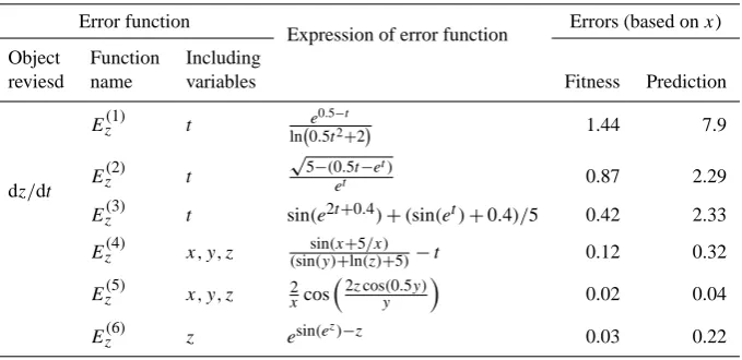
shows that the structural errors of a prediction model can be adjusted by correcting its different components of the model. Similar error corrections have been implemented for the third function Lz(x, y, z). The results are listed in Table 3 and shown in Fig. 5. The effects of the corrections are similar with those of the other two components in the Lorenz model. Based on these results, it can be concluded that various forms of error function can be obtained by the EM algorithm. Some of them are simple error function forms, which may be almost identical to the original error function in the inaccu-rate equation; however, there are also complex forms, which contain various kinds of compound functions. In certain time range, they provide similar dynamic characters. In summary, the information of the prediction error contained in the obser-vation data can be effectively extracted by EM. EM provides a variety of possible forms of error function, which can be used to largely reduce the prediction error in a certain time limit.
4 Conclusions
The development of a numerical model largely depends on the continued improvement of the model and the quality of observational data. The dynamical methods have already be-come an important research direction in climate prediction. The dynamics-statistics approach is a significant and effec-tive way to improve prediction capabilities under the condi-tions of existing models and data. Different from the simple
- 2 0 - 1 0
0 1 0 2 0 1 0 2 0 3 0 4 0 5 0
- 2 0 - 1 0
0
1 0 2 0
0 1 0 0 2 0 0 3 0 0 4 0 0 5 0 0 6 0 0 7 0 0 8 0 0
1 0 2 0 3 0 4 0 5 0 X X 0
X f o r E z ( 1 ) X f o r E z ( 2 ) X f o r E z ( 3 )
(b )
Z
Z0
Z f o r E z ( 1 ) Z f o r E z ( 2 ) Z f o r E z ( 3 )
(a )
X
X 0
X f o r E z ( 4 ) X f o r E z ( 5 ) X f o r E z ( 6 )
Z
n
Z 0
Z f o r E z ( 4 ) Z f o r E z ( 5 ) Z f o r E z ( 6 )
(c )
(d )
Fig. 5. Error correction based on the third componentLz(x, y, z) using EM. (a) and (b) are the fitting and prediction data of the corrected models using the error function Ez(1), Ez(2), Ez(3), respectively. (c) and (d) are the same as (a) and (b), but for E(z4), E(z5), Ez(6), respectively.
statistical correction strategy, this paper proposes a direct correction method of model error based on the EM algorithm, which can make use of dynamic regularities inherent in his-torical data.
In comparison with the original prediction equation, the numerical results indicate that prediction errors are signifi-cantly reduced after the correction by the EM algorithm and the feasibility and ability of the correction scheme proposed in this paper. The present work demonstrates that, using the EM algorithm, the abundance of information present in his-torical data can be used to correct model errors. The present method can make full use of the advantages of dynamics and statistics.
Various forms of error function can be obtained by EM al-gorithm, and it will be a difficult task to choose an appropri-ate equation in application. An ensemble forecasting method can be used to deal with this problem. Based on the predic-tion errors of the model corrected by EM, the proporpredic-tion of the prediction results of the different revised model can be quantitatively allocated. It can reduce the uncertain of the prediction results by the revised model as well as avoiding randomicity of a single revised model.
Table 3. Error functions and errors of the equations obtained by EM (for variabley).
Error function
Expression of error function Errors (based onx) Object Function Including
reviesd name variables Fitness Prediction
dy/dt
E(y1) t sin(sin(t )+sin(t+2))+0.5 4.58 2.45
E(y2) t
4 √
10t2 2.28 7.60
E(y3) t cos(0.5t+tsin(t ))+0.642 0.96 3.74
E(y4) y, z e
√
5
y−√zt−√yt /1.5 0.03 0.22
E(y5) x, y, t (sin(cos(x))+
√
yt )/5 0.04 0.25
E(y6) x, y, z cosxy− 1 2 ln(2z)+y−5)
0.02 0.08
Table 4. Error functions and errors of the equations obtained by EM (for variablez).
Error function
Expression of error function Errors (based onx) Object Function Including
reviesd name variables Fitness Prediction
dz/dt
Ez(1) t e0.5−t
ln 0.5t2+2 1.44 7.9
Ez(2) t
√
5−(0.5t−et)
et 0.87 2.29
Ez(3) t sin(e2t+0.4)+(sin(et)+0.4)/5 0.42 2.33
Ez(4) x, y, z (sinsin(y)(x++ln5(z)/x)+5)−t 0.12 0.32
Ez(5) x, y, z 2xcos
2
zcos(0.5y) y
0.02 0.04
Ez(6) z esin(e
z)−z
0.03 0.22
for the improvement of prediction precision. In future work, the idea presented in this paper will be gradually applied to higher dimensional ordinary differential and partial differ-ential equations. The ultimate goal is to apply the present method to a variety of numerical prediction models.
Currently, EM can be optimized by means of parallel com-puting or cloud comcom-puting. It can be realized by implement-ing multithread parallel computimplement-ing not only for the correc-tion of model errors of single dynamic equacorrec-tion but also for that of multi-equations. Based on this, the computational ef-ficiency of EM can be improved greatly. In fact, the numer-ical calculations used in this paper all are based on multi-core multi-threaded algorithms, which obviously improves the computational efficiency of EM. So we believe that the present study could be applied to more complex systems for the correction of model errors including the model errors of large-scale numerical prediction models.
Acknowledgements. The authors thank the anonymous review-ers and the editor for helpful suggestions, and thank Zuojun Yu in Hawaii University for improving the English in our manuscript. This research was jointly supported by the National Natural Science Foundation of China (Grant No. 41005041), National Basic Research Program of China (973 Program) (2012CB955902), the National Natural Science Foundation of China (Grant No. 40905034), and the Special Scientific Research Fund of Meteorological Public Welfare Profession of China (Grant Nos. GYHY201106015 and GYHY201106016).
Edited by: S. Vannitsem
References
B¨ack, T., Hammel, U., and Schwefel, H. P.: Evolutionary compu-tation: Comments on the history and current state, Evolutionary Computation, IEEE Trans. Evolut. Comput., 1, 3–17, 1997. Cao, H. X.: Self-memorization Equation in Atmospheric Motion,
Sci. China, 23, 104–112, 1993.
Cao, H. X., Kang, L., Chen, Y., and Yu, J.: EM of systems of or-dinary differential equations with genetic programming, Genet. Program. Evol. M., 1, 309–337, 2000.
Chou, J. F.: Short Term Climatic Forecast: Present Condition, Prob-lems and Way Out (I), Bimonthly of Xinjiang Meteorology, 26, 1–4, 2003a (in Chinese).
Chou, J. F.: Short Term Climatic Forecast: Present Condition, Prob-lems and Way Out (II), Bimonthly of Xinjiang Meteorology, 26, 1-4, 2003b.
Chou, J. F.: An Innovative Road To Numerical Weather Prediction – From Initial Value Problem To Inverse Problem, Acta Meteorol. Sin., 65, 673–682, 2007 (in Chinese).
D’Andrea, F. and Vautard R.: Reducing systematic errors by empir-ically correcting model errors, Tellus, 52A, 21–41, 2000. Duan, W. and Zhang, R.: Is model parameter error related to a
sig-nificant spring predictability barrier for El-Nino event?, Result from Theoretical Model, Adv. Atmos. Sci., 27, 1003–1013, 2010. Feng, G. L., Dong, W. J., Li, J. P., and Chou, J. F.: On the stability of the difference scheme in the self-memorization model, Acta Phys. Sin., 53, 2389–2395, 2004 (in Chinese).
Ferreira, C.: Gene expression programming: A new adaptive algo-rithm for solving problems, Complex Syst., 13, 87–129, 2001. Gu, Z. C.: On the utilization of past data in numerical weather
fore-casting, Acta Meteorol. Sin., 29, 176–186, 1958 (in Chinese). Holland, J. H.: Adaptation in natural and artificial systems, Ann
Arbor MI, University of Michigan Press, 1975.
Keller, J. B.: Inverse problems, Amer. Math. Monthly, 83, 107–118, 1976.
Klinker, E. and Sardeshmukh, P. D.: The diagnosis of mechanical dissipation in the atmosphere from determinalarge-scale balance requirements, J. Atmos. Sci., 49, 608–627, 1992.
Lavrentiev, M. M., Avdeev, A. V., and Priimenko, V. I.: Inverse Problems of Mathematical Physics, Berlin, Walter de Gruyter, 2003.
Li, J. P. and Chou, J. F.: Existence of atmosphere attractor, Sci. China, 40, 215–224, 1997.
Li, J. P. and Ding, R. Q.: Temporal-spatial distribution of atmo-spheric predictability limit by local dynamical analogues, Mon. Weather Rev., 139, 3265–3283, 2011.
Li, J. P. and Wang, S. H.: Some mathematical and numerical issues in geophysical fluid dynamics and climate dynamics, Commun. Comput. Phys. 3, 759–793, 2008.
Lorenz, E. N.: Deterministic nonperiodic flow, J. Atmos. Sci., 20, 130–141, 1963.
Lorenz, E. N.: A study of the predictability of a 28 variable atmo-spheric model, Tellus, 17, 321–333, 1965.
Lorenz, E. N.: Atmospheric predictability as revealed by naturally occurring analogues, J. Atmos. Sci., 26, 636–646, 1969. Mu, M., Duan, W., Wang, Q., and Zhang, R.: An extension
of conditional nonlinear optimal perturbation approach and its applications, Nonlin. Processes Geophys., 17, 211–220, doi:10.5194/npg-17-211-2010, 2010.
Qiu, C. J. and Chou, J. F.: A new approach to improve the numerical weather prediction, Sci. China, 31, 1132–1142, 1988.
Saiedian, H.: An evaluation of extended entity-relationship model, Inform. Software Tech., 39, 449–462, 1997.
Schubert, S. D.: A statistical–dynamical study of empirically deter-mined modes of atmospheric variability, J. Atmos. Sci., 42, 3–17, 1985.
Vannitsem, S. and Toth, Z.: Short-term dynamics of model errors, J. Atmos. Sci., 59, 2594–2604, 2002.