Information-theoretic methods for modularity in engineering design

(1)

Information-Theoretic Methods for Modularity in

Engineering Design

Thesis by

Bingwen Wang

In Partial Fulfillment of the Requirements for the Degree of

Doctor of Philosophy

California Institute of Technology Pasadena, California

2007

(2)

c

(3)

Acknowledgements

First of all, I am very grateful to my advisor, Professor Erik K. Antonsson, for his guidance, en-couragement, full support, and patience. He always gave me much freedom to explore what I am interested in and learn the things I enjoy. This made my study at Caltech a pleasant experience. Without his support and advice, I wouldn’t have chance to explore information theory and therefore this thesis would be impossible.

Thanks to Professor Robert J. McEliece, who inspired me in the field of information and coding theory. He always has new ideas and innovative ways to approach different subjects. I have learned much from his inspiring ideas, expertise and research attitude. Also I would like to thank my other committee members–Professor Joel W. Burdick, and Professor Ken Pickar for their support and helpful discussions.

(4)

Abstract

Due to their many advantages, modular structures commonly exist in artificial and natural systems, and the concept of modular product design has recently received extensive attention from the en-gineering research community. Although some work has been done on modularity, most of it is qualitative and exploratory in nature, and little is quantitative. One reason for this gap is the lack of a clear definition of modularity. This thesis begins with a detailed discussion on the concepts of “modularity” and “module”.

Based on the background presented here, a mutual information-based method is proposed to quantify modularity. The method is based on the view that coupling is information flow instead of real physical interactions. Information flow can be quantified by mutual information, which is based on randomness (or uncertainty). Since most engineering products can be modeled as stochastic systems and therefore have randomness, the mutual information-based method can be applied in very general cases, and it is shown that the commonly existing linkage counting modularity measure is a special case of the mutual information-based modularity measure.

The mutual information-based method is applicable to final design products. But at the early stage of the engineering design process, there are generally only function diagrams. To exploit the benefits of modularity as early as possible, a minimal description length principle-based modularity measure is proposed to determine the modularity of graph structures, which can represent function diagrams. The method is used as criteria to hierarchically decompose abstract graph structures and the real function structure of an HP printer by evolutionary computation. Due to the specialty of genome representations in evolutionary computation, new genetic operators are developed to determine optimal hierarchical decompositions.

(5)

List of Figures

1.1 An ambiguous image: Eskimo or Indian. . . 2

1.2 Executive offices of the president of the U.S. . . 3

1.3 Modular structures in airplane and CPU. . . 3

1.4 Non-modular truss structure synthesized automatically by MOSS [96] . . . 5

2.1 Market value of the U.S. computer industry [3] . . . 14

2.2 Modularity reduces redundancy. . . 15

2.3 The modeling of a system. Modularity1 _{is not well-defined. Modularity}2_{= Modularity}3_{. 20} 2.4 A simple Ising system. . . 22

2.5 Relativity of interactions. . . 23

2.6 The levels of hierarchy. . . 23

2.7 The effects of modularity at different levels on the overall modularity. . . 24

2.8 Different decompositions. . . 27

2.9 Structures of neural networks. . . 28

2.10 Different types of landscapes. . . 29

3.1 Relationship between entropy and mutual information . . . 35

3.2 Mutual information as a measure of coupling of two systems of random variables. . . . 38

3.3 Random system of example 3.3.1. . . 41

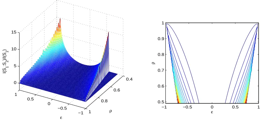
3.4 The coupling between bivariate normal variables. . . 42

3.5 I(S1:S2) vs. ρandǫ: the right is contour plot. . . 42

3.6 C1_vs. _ǫ_and_ρ_{. . . .} ₄₅

3.7 A hierarchical structure. . . 46

3.8 A model of two-way clustered stochastic systems . . . 49

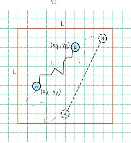
3.9 Two particles on a lattice. . . 50

3.10 Posterior probability of (XA, YA). . . 51

3.11 Mutual information vs. the length of link connecting the two particles. . . 52

3.12 How much information need to be communicated? . . . 53

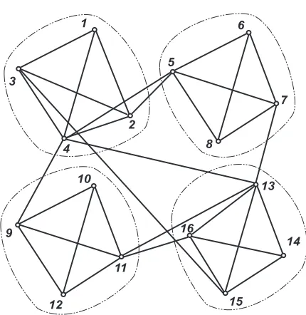
3.13 Probability distribution ofdv and dc in example: fit interdependency. . . 54

(9)

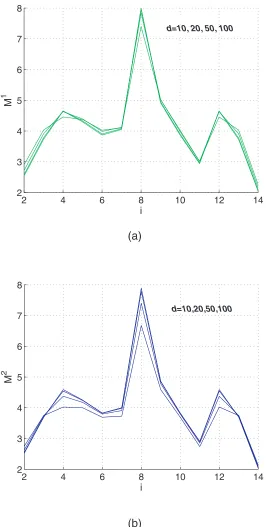
3.15 Effects of the diagonal elementdonM1_{, M}2_{. . . .} ₅₇

3.16 Effects of vertex ordering onM1_{, M}2_{. . . .} ₅₈

4.1 Modularity is a kind of regularity. . . 65

4.2 Modularity at different levels. . . 67

4.3 An example graph representation and its hierarchical tree representation. . . 69

4.4 A simple example for information measure of modularity of graph structures. . . 75

5.1 Graph representation of a function structure. It’s a function structure of an HP 1200C desktop inkjet printer from K. Otto and K. Wood’s Product Design [70] . . . 79

5.2 General structure of genetic algorithm. . . 80

5.3 Tree representation of hierarchically modular structures. . . 81

5.4 Crossover step 1: genome structures of initial parents. . . 82

5.5 Crossover step 2: select crossover points. . . 83

5.6 Crossover step 3: delete repeated leaves. . . 84

5.7 Crossover step 4: add subtrees. . . 84

5.8 Crossover step 5: clean fragments. . . 84

5.9 Mutation: swapping two leaves. . . 85

5.10 Mutation: swapping two subtrees. . . 85

5.11 Mutation: merging single nodes into other subtrees. . . 85

5.12 Mutation: merging single nodes as a subtree. . . 86

5.13 Mutation: merging two subtrees. . . 86

5.14 Mutation: splitting a subtree. . . 86

5.15 Decomposition result for example 1. . . 88

5.16 GA convergence of mutual information-based measure for example 1. . . 88

5.17 The effect ofdon the fitness (modularity) of the best individuals in example 1. . . 89

5.18 GA convergence of MDL-based measure for example 1. . . 89

5.19 Decomposition result for example 2. . . 90

5.20 GA convergence of mutual information-based measure for example 2. . . 90

5.21 The effect ofdon the fitness (modularity) of the best individuals in example 2. . . 91

5.22 GA convergence of MDL-based measure for example 2. . . 92

5.23 Function structure decomposition: (a) The abstract graph representation of the func-tion structure of HP1200C. E: power; e: human energy; s: signal; p: paper; I: ink; h: heat; a: air. (b) One decomposition found by the algorithm. . . 92

(10)

6.1 An example of artificial neuron. . . 98

6.2 Multi-layer artificial neural network. . . 98

6.3 An example decomposition for modularity measure. . . 102

6.4 The structures of neural networks used in experiment 1. . . 103

6.5 The learning errors for networks with fixed number of links. . . 103

6.6 The structures of neural networks used in experiment 2. . . 104

6.7 The learning errors for networks with 20 hidden nodes. . . 105

6.8 The learning errors for networks with 14 hidden nodes. . . 105

6.9 Algorithm used in experiment 2. . . 106

6.10 Results of evolving networks with 20 hidden nodes. . . 107

6.11 Algorithm used in experiment 3. . . 108

6.12 Results of evolving networks with fixed number of links. . . 109

(11)

List of Tables

4.1 Code lengths for units in case without decomposition. . . 74

4.2 Code lengths for units in case without decomposition. . . 75

4.3 Code lengths for units inM1. . . 76

4.4 Code lengths for interfaces inM1. . . 76

4.5 Code lengths for units at level 1. . . 76

(12)

Chapter 1 Introduction

1.1 The Ubiquity of Modularity

Modularity is all around us:

• In Figure 1.1, you can see an Indian looking towards you or an Eskimo with his back to you looking into a cave, but you can’t see them both at the same time because our minds have “temporal modularity” [76]. That is, different computational configurations of nerve systems cannot exist contemporaneously.

• Neuroscientific evidence [31, 66] shows that there are two distinct cortical pathways in human brains for “where” and “what” tasks. Nervous systems have a ventral (temporal) pathway for recognizing the identity of an object and a dorsal (parietal) pathway for identifying its location.

• In biological evolution processes, it took about three billion years for nature to evolve single-celled organisms to multi-single-celled organisms while it only took about five million years to evolve from multi-celled organisms to now existing mammals. Why did it take so long for single-celled organisms to evolve into multi-celled organisms? One reason appears to be that modularity

hastens the evolution process. Modularstructures can lead to rapid adaptation to environments because by adding, subtracting, or modifying submodules, incremental changes can be more quickly tried and either adopted or rejected.

• There are a small number of kinds of single-celled organisms, while there are thousands of billions of organisms existing now in the earth. This is also due to theirmodular structures.

Modular structures can exponentially increase variety.

(13)

Figure 1.1: An ambiguous image: Eskimo or Indian.

• Social structures and organization structures in human activities are modular. For example, themodular organization structure of the Executive Office of the President of the is shown in Figure 1.2

• People adopt modular methods to tackle complex problems. This modularity is mainly due to people’s limited short-term memory, which is key to solving many intellectual problems. Because of this limitation, people can only handle one relatively small and easy problem at a time. This makes people decompose a complex problem into subproblems, therefore in a modular way.

• Many engineering designs are modular, probably due to people’s modular way of tackling complex systems. A Boeing 747-400 has six million parts, and Pentium 4 has as many as 55 million transistors. As shown in Figure 1.3, they both are modular. It is their modular

structures that make such complex systems manageable.

• Computer programming languages have evolved from structural languages like Basic, Fortran to C++ and object-oriented programming. It is thismodular design methodology that makes it possible to develop large and complex applications.

• This thesis is also modular. First the structure ismodular. It has chapters, and each chapter has sections, which contain subsections. Second it’smodular in semantic sense. Each chapter has relatively independent contents.

(14)

National Security Council

National Economic Council

Domestic Policy Council

Science, Technology and Space

Environmental Policy

National Drug Council Policy Development Offices

Office of Administration

Executive Residence U.S. Trade Representative

Office of Vice President Office of the

President Economic

Advisers

Office of Management

and Budget

THE PRESIDENT

Figure 1.2: Executive offices of the president of the U.S.

(15)

• This list is modular with a collection of independent facts and observations organized into bulleted points.

The commonality of all of the elements in the above list is theirmodularity. As listed above, mod-ular structures are widely employed in artificial and natural systems, and modmod-ularity is a necessity for the development of highly complex systems and a critical issue in understanding large complex systems. The universality of modularity is mainly due to its many advantages such as expanding humankind’s limited intelligence capabilities to manage complex systems by making large systems more manageable, reducing cost [85], increasing flexibility [3, 85, 100], and boosting the rate of innovation [3]. The benefit of modularity will be discussed in more detail in section 2.2. Due to its wide use, its importance for understanding complex systems, and many advantages, modularity has recently received a lot of attention in many different fields, such as engineering design [3, 98, 100], production and manufacturing [67, 92], industrial infrastructure [58, 86], artificial intelligence [11], neural computation [5, 12, 32, 36], software engineering [74, 73], robotics[7, 43], brain science [50, 82], and biological evolution [8, 13, 101, 102].

1.2 Motivation: The Ambiguity and Informality of

Modu-larity

Though the terms “modular” or “modularity” are used throughout the engineering literature, little empirical or even theoretical work has been done in either measuring or quantifying the modularity of artificial or natural systems. One reason for this gap is the lack of a clear definition of modularity. Even though the literature offers some definitions for modularity in different fields from different views, there seems to be no unified view on such questions as what exactly modularity is and what determines a “module.” So, it is necessary to clarify the concepts of “modularity” and “module” in order to take advantage of modularity to provide good guidelines for synthesizing modular structures or products.

(16)

Figure 1.4: Non-modular truss structure synthesized automatically by MOSS [96]

synthesize modular structures, such as a truss. The example shown in Figure 1.4 is one automat-ically synthesized by MOSS, a computer program [96]. The structure is highly non-modular. It is necessary to propose a quantitative modularity measure to help synthesize modular structures.

1.3 Chapter Overview

In this work, the definition of modularity is clarified first, then information-theoretic measures for modularity are developed, and then are verified as criteria to decompose graph structures and function structures in engineering designs. At last, they are used to evolve modular artificial neural networks.

In the thesis, properties and definitions of “modularity” and “module” are qualitatively discussed in Chapter 2. A framework of mutual information-based measures of modularity is proposed in Chapter 3, and the framework can be used to quantify modularity of dynamic behaviors in stochastic systems, design processes, manufacturing and other processes. Minimal Description Length (MDL) principle-based measures for structural modularity of graph structures are discussed in Chapter 4. Chapter 5 uses the measures to decompose graph structures and function structures in engineering design, and Chapter 6 presents preliminary studies on how to evolve modular topology structures of artificial neural networks.

1.4 Contributions Made in the Thesis

The thesis contributions are listed below:

(17)

2. Information flow is introduced as a quantification of interactions between systems. Based on the information theoretic view, a mutual information-based measure is proposed as a quantitative measure of modularity. The information-theoretic measure can be applied to more general systems than those real physical interaction-based methods, and it is shown that the existing linkage counting methods are a special case of the mutual information based method. See Chapter 3.

3. Since the mutual information-based method is limited to existing devices or systems, an MDL-based modularity measure is proposed for structure modularity of graph representations, which is common at the early phase of engineering design. See Chapter 4.

4. These information-theoretic methods are demonstrated by being used as criteria to hierar-chically decompose abstract graphs and function structures. New genetic operators for tree representations of modular structures are developed in evolutionary computation, which is used to hierarchically decompose graph structures by evolutionary computation according to the information-theoretic measures. See Chapter 5.

5. The aim of developing quantitative modularity measures is to produce modular engineering products. To evolve modular structures, the first step is to understand the factors that will affect the synthesis of of modular structures by evolutionary design. The thesis preliminarily studies the effects of the modularity of tasks on the modularity of structures generated by evolutionary computation and shows that the effects are task and resource dependent. See Chapter 6.

1.5 Design as an Evolutionary Process

Engineering design is discussed from the perspective of biological evolution in this section. Compar-ing design processes to natural evolution will help to understand the benefits of modularity, origins of modules, formation of modular structures, and to develop modularity measures.

1.5.1 Design Space

(18)

color. Let’s denote the set of design parameters as (x1, x2,· · · , xn), and supposexitakes some value from domain Ri. Domain Ri could be an interval inR, such as the height of cylinder, or it also could be a discrete value from a set, such as the color. Then, thedesign space can be thought of as

R1×R2× · · · ×Rn. Any specific design can be viewed as a point in the design space.

1.5.2 Design Evolution

Biological evolution is a process where individuals with high fitness survive in a complex environment to pass their traits on to offspring. The traits of the offspring are determined by a mix of the parents genes (through crossover) and mutation. The evolution trajectory of an organism can be viewed as one in the evolution landscape, in which the altitude of the point equals the fitness of the organism. As an analogy to biological evolution, consider there is a landscape in design space. During design processes designers create variations of designs by changing design parameters, and move from one point to another in the landscape. Given adequate knowledge of determining where to move and the ability to move around in the landscape, designers could drive designs upward toward higher altitudes.

To formally describe design evolution, the following things are needed:

1. A design space which includes many designs (entities) and where designers can explore design alternatives.

2. A fitness measure, which the selection of modular design configurations is based on.

3. Sources of variation, which can explore many designs in the design space. A variation can happen to one design (entity) and produce a new one, like mutation operators in biological evolution, or it could happen to several entities and produce several new entities, like crossover operators which produce one or more new entities from two existing ones.

4. Mechanisms of selection, which include criteria to choose designs (entities) for the next genera-tion (or iteragenera-tion of the design process. In some contexts, selecgenera-tion mechanisms are two-valued functions. One value represents keeping a design (entity) for the next generation, and the other one means throwing away a design (entity).

5. Control units which control sources of variation and selection mechanisms. In typical design process, designers are the control unit, and their counterparts in biological evolution are com-plex environments affecting selection mechanism and mutation and reproduction processes controlling crossover and mutation.

(19)

Definition 1 (Fitness Landscape) A fitness landscape L is a triple L =hD, R, fi, where D is the design space, R ⊂ D×D is a neighborhood relation on D, and f : D −→ R _{is a fitness (or}

objective) function.

Peaks in a landscape are defined as:

Definition 2 (Peak) A point x ∈ D is a local peak if f(y) ≤ f(x),∀yRx and a global peak if

f(y)≤f(x),∀y∈D.

With the definition of a fitness landscape, design evolution (process) can be defined as:

Definition 3 (Design Evolution) A design evolution E is a quadruplehL, V, S, Ci, where

• L is a fitness landscape hD, R, fi.

• V is a set of variation operators which are mappings fromDm _to_Dn_{, m, n}_∈_N_.

• S is a selection mechanism, which is a mapping fromD to{0,1}.

• C represents a set of control rules.

1.5.3 Difference between Design Evolution and Biological Evolution

Despite the strong parallels between biological and design evolution, the following differences are important to observe.

1. Moving around in the landscape in design evolution is not totally random since designers, the fundamental control units of design evolution, are capable of seeing and seeking values in design spaces while they are random in biological evolution. This is a key reason why organisms evolve much more slowly than engineering designs.

2. Biological selection pressures are on the whole systems, i.e., the combined genotypes and phe-notypes.1 _{Whereas in modular structures, design evolution can select for specific subsystems}

or modules.

3. The fitness landscape and evolution spaces can both vary with time in biological evolution and design evolution. Yet the speeds of changes in design evolution are much faster than those in biological evolution.

4. In design evolution, designers are the only control units, while in biological evolution, selection mechanisms and variations are probably controlled by different units. The variation sources in biological processes are reproduction processes which are controlled by some mechanism

1

(20)

(21)

Chapter 2 Qualitative Modularity

2.1 Introduction

Due to their importance in understanding and managing complex systems, modular structures are favored in engineering practice. In order to produce modular structures, engineers need to under-stand the following questions: What is modularity? What is a module? And what characterizes modularity? Then a quantitative measure of modularity is needed. These are motivations for this thesis work.

Though there are already many qualitative discussion of modularity [3, 46, 61, 81, 85, 86, 100](refer to Section 2.4), they are not yet unified and there are still some very basic questions related to basic properties and quantitative measure of modularity that need to be clarified. This chapter mainly discusses those questions after a detailed discussion of the benefits and costs of modularity and a survey on existing views of the definition of modularity.

2.2 Benefits of Modularity

2.2.1 Product Evolution

In nature, single celled organisms dominated the Earth for billions of years. Multi-cellular organisms came into existence only about 500 million years ago. In mere tens of millions of years, they evolved so rapidly that they overtook three billion years of evolution of the single-celled organisms, replacing them as the dominant living things. The main reason for this is the modular structures of organisms. As discussed in Chapter 1, there are similarities between engineering design and biological evolution. Modular structures can also hasten product evolution and produce better performing designs. What is the real mechanisms behind these benefits? Based on the elements of the design evolutionE=hL, V, S, Ci, modular structures can speed up the development process by:

(22)

in-terconnected to K(K < N) other components. The neighborhood relation R, i.e., the K

connections for every component, can be chosen randomly. With the value ofK varying from 0 to N −1, the system changes from totally decomposable to wholly integral. The config-uration (or state) space X is {0,1}N_{, and the fitness function is the average of the fitness} values, fi, of each of the N individual components. The fitness value, fi, of component i

is determined by the configurations (or states) of itself and its K neighborhood components

{xi1,· · ·, xiK}, {i1,· · · , iK} ⊂ {1,2,· · ·, i−1, i+ 1,· · · , N}. That is,

f(x) = 1

N

X

i=1

fi(xi, xi1,· · ·, xiK), (2.1)

wherefiis a randomly generated mapping from{0,1}K+1to (0,1). Then, the fitness landscape ishX, R, fi. The results in Kauffman [53, 54] showed that

– ForK= 0, there is only one peak in the fitness landscape.

– ForK=N−1, the expected total number of local peaks is _N2N₊₁.

– ForK large, the average Hamming distance1_{between local peaks is approximately}

Nlog(K+ 1) 2(K+ 1) .

Those results imply that withN fixed, asKincreases, i.e., the modularity decreases, the total number of local optima increases to a large number, and the landscape becomes increasingly rugged.

• Parallelizing the tasks or processes: The clear and well-defined interfaces of modules can enable design tasks to be decoupled, and every module has a well-defined function, therefore it is feasible to define a fitness function on the module, which makes design evolution possible on module levels. This decoupling results in the ability to complete tasks in parallel.

• Reducing design spaces: While decomposable structures can split the design space into several small ones and evolve on module levels, non-decomposable but not wholly integral systems can reduce the design spaces, though they can not split design spaces. Due to the reduced design space, modularity also boosts the rate of innovation [4], and leads to rapid trial-and-error learning [58].

• Making people (controllers) work more efficiently: People can only consciously work with a limited number of concepts at any time. Short-term memory, which is you used when solving an intellectual problem, only holds six or seven items [64]. This drives people to be specialized and solve problem in modular ways, and therefore they are more efficient in design.

1

(23)

2.2.2 Production Variety

As to be discussed in Section 2.6, a module usually has well-defined interfaces and realizes some spe-cific functions, and standard interfaces and well-defined functions of modules make it exchangeable. Usually there are several alternative components which can implement a functional element. The existence of alternative options makes it possible to construct a large variety of end products from a much smaller set of different components.

Simon [90] pointed out that “the more complex arise out of a combinatoric play upon the simpler. The larger and richer the collection of building blocks that is available for construction, the more elaborate are the structures that can be generated.”

Suppose a system is composed ofmmodules and every module hasni, i= 1,· · ·, malternatives, respectively. Then, by the multiplication principle, ideally there areQm

i=1ni realizations. It is easy see that the number of combinations expands exponentially with respect to the number of modules. Though this exponential expansion would not happen in practice, modular structures can provide many options for production development. For example, IBM was able to create seven different printer motors by varying only face plates, gears, and end caps of the motor while leaving 25 other parts unchanged [100].

2.2.3 Cost Saving

The cost of designs includes development cost, test cost, and maintenance cost. All of those costs can be reduced by modularity. Firstly, a module has well-defined functions, and its interfaces are standardized so that its interactions with the rest of the product are minimized. This standardization allows the same component (module) to be used across product lines. This component sharing can dramatically reduce development costs.

Another cost saving factor is differential consumption [100]. Different parts of systems possibly have different consumption rates and require different materials, e.g., tires of automobiles. Mod-ularity makes it possible to separate those parts from the rest of a system, and this strategy can drastically reduce the cost of the other “non-consumable” parts which otherwise have to be replaced with the same rate as consumable parts, and therefore, maintenance cost. Another maintenance cost saving factor is that maintenance can happen locally in modular structures in the sense that you can maintain modules separately.

(24)

fraction of all possible combinations are tested, and usually the number of tested cases is proportional to the total number. The following discussions on the extreme case will still provide some sense of test cost savings in modular structures.

One scenario is an integral design, and the other is decomposable design, which has two modules, with each having ntest parameters. In the integral design, the system behavior is decided by the whole set of the test parameters, so the test can not be divided into different tests on subsets of the test parameters. Then, the possible number of tests is the total number of combinationss2n _.

In the decomposable design, since each module has a well-defined function, the test on the whole system can be divided into two tests on the two modules, respectively. Then, each hassn _possible test combinations, so there are 2sntests on module levels. How about integration tests on the system level? Let’s assume each module has m output states, which is much smaller than the number of its possible state configurations, i.e.,m≪sn_{. Then, the number of system level tests is} _m2_{, so the}

total number of tests is 2sn₊_m2 _≪_s2n_.

2.2.4 Specialization

Decoupling of production and design tasks of modular products enables individuals or firms to increase specialization [57]. Figure 2.1 shows the specialization in the computer industry due to the emergence of modular structures in computer architectures.

Specialization makes people concentrate their productive efforts on a rather limited range of tasks and encourages them to pursue specialized learning curves, increase their differentiation from competitors [86], and focus on a narrow area of knowledge, skills or activities. Specialization drives individuals or firms to have unusually effective or efficient performance of some particular function and increase their productivity and the reliability of products.

2.2.5 Reliability

(25)

Category definition

Computer and Office Equipment Except IBM Electronic Components and Accessories Semiconductors and Related Devices Computer Peripheral Devices Electronic Connectors Computer Ternimals

Computer Processing, Data Preparation and Processing Electronic Computers

Computer Integrated Systems Design Computer Storage Devices

Prepackaged Software

Computer Communication Equipment Printed Circuit Boards Computer Programming Other Services Printed Circuit Boards Computer Programming Services Computer Leasing

Start date 1960 1960 1960 1962 1965 1968 1970 1970 1970 1971 1973 1974 1974 1974 1974 1974 Code

3570 3670 3674 3577 3678 7374 3571 3575 7373 3572 7372 3576 3672 7370 7371 7377

(26)

0 0.1 0.2 0.3 0.4 0.5 0.6 0.7 0.8 0.9 1 0

1 2 3 4 5 6 7 8 9 10

Factor failure probability (p)

PA /PB

n=2 n=3 n=5 n=10 n=∞

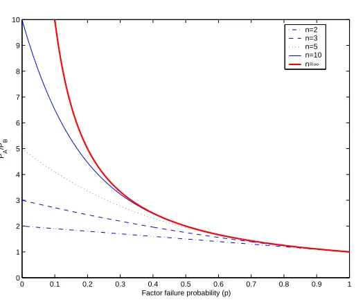
Figure 2.2: Modularity reduces redundancy.

• In the non-modular structureA,

PA= 1−(1−p)n. (2.2)

• In the modular structureB,

PB=p. (2.3)

Figure 2.2 shows the relation betweenPA andPB.

It can be seen from Figure 2.2 that the smallerp, the more benefits modular structures can gain. Usually in engineering,pis quite small, soPA can be approximated by a Taylor expansion:

PA= 1−(1−np+o(p)) =np+o(p)≈np (2.4)

And then

PA

PB ≈

np

p =n (2.5)

In another limit case: n→ ∞, thenPA→1, and therefore P_PB_A = 1_p.

This may partially explain why natural neural systems utilize a redundancy factor of 10,000 while current electronic systems use a factor of 2 to achieve very high reliability? The structures of neural systems are not so modular compared to modern electronic systems.

2.3 Cost of Modularity

(27)

into subsystems (or modules). As shown in the evolution of computer architectures, before the highly modular system of today, the first general purpose computer “ENIAC” was highly interconnected and non-modular [4].

Performance is usually not optimal in modular structures. Given unlimited engineering resources, some performances of any particular product can be improved by reducing modularity. The per-formance improvement is often in terms of reduced size and mass. Modular designs can contain redundant physical structures and do not exploit as much function sharing2 _{as possible.}

Modularity may also increase some costs by introducing some redundancy and using standard components. When standard components are used in some particular applications while they are designed for more general applications, they may have excess capability.

Modularity can make products excessively similar by using standard components. Some auto makers have suffered from this problem because of the customer perception of too much sharing of styling and systems across models [100]. For this reason, much of the standardization of components that can be achieved with modularity is confined to hidden components, particularly in consumer goods [71].

2.4 Brief Survey on Definitions of Modularity

Due to the benefits discussed in the previous section, modularity became an important concept in engineering design. However, the concept of modularity and modular methods or structures are not new at all. The modular strategy originated very early. In the 1640s, in his“A Discourse on Method: Meditations on first Philosophy,” [17] Rene Descartes, the French philosopher and mathematician, proposed a modular method using decomposition as one of the basic ways to solve problems: “... to divide each of the difficulties under examination into as many parts as possible, and as might be necessary for its adequate solution...” The practice of modular strategies in engineering is also very early. In the 1900s, the Wright brothers used a modular design method to invent the airplane. They tackled the problem by solving three separate subproblems: lateral control, lift, and propulsion. To some extent, it was a modular design method that enabled their success [47]. The modular production paradigm in production is also very old. In 1914, Swan [95], an automotive engineer, extended the standardization idea across production and for large components, standardizing wheel sizes, hubs, bearings, axles, and fuel feeding mechanisms. Producing final products by assembling standard components dominated the early history of the U.S. auto industry through 1930.

In the 1960s, Alexander [1] and Simon [90] systematically studied methods to design complex systems and analyze their behaviors. In “The Architecture of Artificial,” Simon [90] discussed a broad ranging set of systems, from business organizations to biological systems, that exhibit

2

(28)

a property of being “nearly decomposable”, and also argued that those complex systems often take a hierarchical form, whereby the system is composed “... of interrelated subsystems, each of the latter being in turn hierarchic in structure until we reach some lowest level of elementary subsystem.” He described nearly-decomposable systems as those where “the short-run behavior of each of the component subsystems is approximately independent of the short-run behavior of the other components,” and “in the long run the behavior of any one of the components depends in only an aggregate way on the behavior of the other components.” Simon suggested that intra-module interactions are stronger than inter-module interactions in nearly decomposable (modular) systems. This view fits well with common intuitions and is widely adopted, but it has limits.

Firstly, only considering the strength of intra-module and inter-module interactions is sometimes overly simplistic when applied to complex dynamical systems. Sometimes the functional behavior of one module is strongly dependent on the inter-module interaction, despite a week interaction [109]. Secondly, it is necessary to consider the “size” of modules (“granularity”). The granularity of modules affects the intra-module interactions, therefore the ratio of intra-module and inter-module interactions.

Considering the effects of the granularity of modules, Wagner [102, 103] introduced function to limit the size of modules, although this view is limited to the field of biology. He provided three criteria for recognizing modular phenotypic units: “(1) collectively serve a primary functional role; (2) are tightly integrated by strong pleiotropic effects of genetic variation; and (3) are relatively independent from other such units.”

Wagner’s view is not the only one which associates modularity with functionality, even in the field of biology. Based on Fodor’s work [21], Elman [18] stated: “A module [of mind] is a special-ized, encapsulated mental organ that has evolved tohandle specific information types of particular relevance to the species.”

In engineering design, Pahl [71] defined modular products as “machines, assemblies, and com-ponents that fulfil various overall functions through the combination of distinct building blocks or modules” and different types of modules to implement different types of technical functions including basic, auxiliary, special, and adaptive.

Ulrich [100] argued modularity depended on two factors – similarity between the physical and functional architectures of designs and minimization of incidental interactions between physical components. A modular architecture includes a one-to-one mapping from functional elements in the functional structure to the physical components of the product and specifies decoupled interfaces between components. An integral architecture includes a complex (non one-to-one) mapping from functional elements to physical components and/or coupled interfaces between components [98].

(29)

suitable for decomposable systems, but not for non-decomposable systems. There are no clear definitions for module with primary functional roles. Furthermore, functionality is not the only aspect of modularity. Modularity is multi-dimension and it also includes other aspects such as physical, temporal, life cycle [67], and design process. For example, modularity in the brain can be categorized into three different types: architectural modularity, functional modularity, and temporal modularity [10]

Another question is on the definition domain of modularity. Some views limit modularity to modular structures. Galsworth [24] viewed modularity as having standardized and interchangeable components: “modular design is a unit or group of standardized elements or parts that may be used within a number of different products.” Baldwin and Clark [4, 3] stated “a modular system is composed of units (or modules) that are designed independently but still function as an integrated whole.” Langlois [57] stated “modularity is about how parts are grouped together and about how groups of parts interact and communicate with one other.” Some other scholars view modularity as a general concept for any system. For example, Shilling [86] viewed modularity as a matter of degree, and “a complex system can be modular at various degrees.”

2.5 Modularity

The general principles or properties of modularity that have been discussed in the literature surveyed in the above section are summarized here:

1. Modularity is a systematic concept and is a global characteristic of a system. 2. Modularity is related to intra-module and inter-module coupling.

3. Modularity is hierarchical. A modular system can be separated into subsystems, and subsys-tems can also be separated into sub-subsyssubsys-tems, and so on.

4. Modularity is multi-dimensional. Modularity is related to many different aspects such as physical structures, function structures, design processes, and time.

5. Modules usually realize some functions.

The following important aspects of modularity have not been discussed in the literature and need to be clarified.

(30)

2. Relativity of Interactions: Modularity compares inter- and intra-module interactions of a sys-tem. Should a modularity measure compare the total quantity of interactions or the interaction “density”?

3. Hierarchy: Modularity is hierarchical. How then is the modularity of a whole system affected by the modularity of its subsystems and aggregated from them?

4. Decomposition: If a system is decomposed, there are no modules or subsystems. Therefore, “inter-module” or “intra-module” is not well defined. That is, what is the specific meaning of “inter-module” or “intra-module”?

5. Definition Domain: Should modularity be limited to modular structures or be a universal concept in the sense that any system can be modular to some degree, and the definition of modularity should work across a broad range of cases?

6. Quantifying Interactions: What is the specific meaning of “couplings”? How to quantify interaction strength?

The first five questions are discussed in the details below, and the quantification of interactions (coupling) will be discussed in the next chapter.

2.5.1 System and Model

A system consists of elements and interactions among the elements. Modularity is used to describe the degree of interactions among the elements. So, modularity is related to the global behavior of a system, and this leads to a number of questions. For example, what should be considered “global behavior ”? What constitutes the overall function of a system? Since the understanding of behaviors of a system depends on observers’ knowledge, how does people’s knowledge affect the modularity of the system?

(31)

System

Observor

Representation

Model

Modeling

Representing

Observing

Framework

Modularity

1

Modularity 2

Modularity 3

Figure 2.3: The modeling of a system. Modularity1_{is not well-defined. Modularity}2_{= Modularity}3_.

limited ways” [26]. The modularity of the mind is objectively there. However our answer changed from non-modular to modular.

In fact, there is no criterion to tell whether your knowledge of a system is complete or not. That is, it is really difficult to tell whether the modularity observed is the real modularity of the system or not. This does not mean, however that it is impractical to talk about modularity, although it is very difficult to directly measure the modularity of a system. Usually, a given system, especially a natural system, has too many contents, and it is impractical or unnecessary to arbitrarily accurately describe it, which is beyond our understanding and modeling abilities. So, the system should be approximately modeled under some framework and formalized by some representation languages, as shown in Figure 2.3. Now the behaviors of models and therefore modularity can be studied. Does this mean the measure of modularity will become subjective? If observers model a system and do activities related to modularity within an established framework, the modularity of the system can be determined with respect to the framework, and different observers’ views on modularity should be consistent.

(32)

whether there is a maximal element in {M odi} under the order ≤. The answer is negative since ordering ≤ is usually not a total one.3 _{Suppose there are two model} _{M od}

i and M odj describing information setsIi andIj respectively, whereIi6=Ij. Unfortunately it’s not guaranteed that there exists another model describing the information setIi∪Ij.

So, when people talk about modularity of a system, they are talking about modularity of a model of the system which is modeled under some default framework.

2.5.2 Multi-Dimensional

Modularity is multi-dimensional. Modularity of a specific aspect could be thought as the projection of the overall modularity. For example, biological modularity can be classified into three aspects: development, morphology, and evolution [13]. In engineering, modularity could include physical structure, function, temporal relationship, life cycles, etc. High modularity in one dimension does not necessarily mean high modularity in another dimension. A system could have strong inter-module dependencies in one aspect, though it may clearly be modular in other aspects. Here is a simple example.

Consider the simple Ising model [110] shown in Figure 2.4. There are 4 spins and connections between them. Each spin has a state 0 or 1, and the digital number over a line is the number of connections the line represents. The dynamic behavior follows the following update rules:

P(Si(t+ 1) = 1) = P 1

j6=icij

X

j6=i

cijSi(t) and

P(Si(t+ 1) = 0) = 1−P(Si(t+ 1) = 1),

wherecij is the number of connections between spiniand spinj, andSi(t) is the status of spiniat timet.

From the structure view, the system can be thought as a modular one, with spin 1 and 2 clustered as moduleM1and spin 3 and 4 clustered as moduleM2. Does the modular structure imply modular

dynamic behavior?

Let’s denote the system state as a four-bit binary expansion (S1S2S3S4). Given the initial spin

state, the dynamic behavior of the Ising model is a Markov chain. From analysis on the transition probability matrix, there are two absorbing status (0000) and (1111), so the stationary state,Sf, of the dynamic system should be either (0000) or (1111). It is not difficult to get that the probability

3

A total ordering≤on a setAis an ordering satisfying the following four properties: 1. x≤y, y≤z⇒x≤z, Transitivity.

2. x≤y, y≤x⇒x=y, Anti-symmetry. 3. x≤x,∀x∈A, Reflexivity.

(33)

D A

B

C 5

5

5 5

5

5 1

M

1

M

2

Figure 2.4: A simple Ising system.

of Sf is uniform, i.e., P(Sf = (0000)) = P(Sf = (1111)) = 0.5 if the probability distribution of initial states is uniform. No matter what the stationary stateSf is, the state of (S1S2), considered

moduleM1, can completely be inferred from the state of (S3S4), considered module M2, and vice

versa. This means that the dynamic behaviors ofM1and M2 are totally coupled.

2.5.3 Relativity of Interactions

While discussing the modularity of a system, it is necessary to compare the inter and intra-module interactions of the system. The weaker inter-module interactions and stronger inter-module in-teractions of a system, the better the modularity of the system. This means that modularity is related to the relative strength of module interactions compared to that of intra-module inter-actions. This relativity makesgranularity, i.e., the “size” of modules, come into consideration while defining modularity. “Size” could be the number of basic units or the amount of information from information-theoretic views. For example, there are two systems,S1andS2, each having two

subsys-tems. The two systems have the same “size” and inter-subsystem interaction strength, but different intra-subsystem interaction strength. S1s subsystems are completely integrated, but S2s are fully

decomposable. If only based on the relative strength of subsystem and intra-subsystem inter-actions,S1 is more modular thanS2, but actually S2 is more modular. In this case it is necessary

to compare the modularity of subsystems, i.e., to decompose the subsystems further.

(34)

Figure 2.5: Relativity of interactions.

1 2

0 A

3 Node Level

1 2 Modularity

Level

Figure 2.6: The levels of hierarchy.

which has three modules at one level, shown in Figure 2.5(c). However, if interaction “density,” interactions normalized out by the “size”of module, is used, then the structure in Figure 2.5(c) will be better than the one shown in Figure 2.5(b).

So, to compare modularity, the interactions need to be normalized out by the “size” of modules, i.e., they become interaction “density”.

2.5.4 Hierarchical

Hierarchical structures are common in complex systems. Complex systems take advantage of the hierarchy to regulate the states and structures of their subsystems, make them operate nearly inde-pendently of each other, and evolve rapidly and easily. The hierarchy looks like a tree. The levels of nodes are increasingly assigned from bottom to root, with the beginning at level 0, and the levels of modularity begin at node level 1, as shown in Figure 2.6.

(35)

Inputs

Inputs Outputs

Outputs

Neural Network Neural Network

(a)

(b)

Figure 2.7: The effects of modularity at different levels on the overall modularity.

levels and define modularity for the units at a specific level. How then does the modularity of units at different levels affect the overall modularity of a model? Modularity of units at different levels of the hierarchy have different effects on the overall modularity. Modularity at a higher levels dominates those at lower levels, and it is not necessary that modularity of subsystems should be less than the overall modularity. For the two neural networks in Figure 2.7, units in the left one are highly integrated, but every unit has a modular structure, and whereas the right one is modular at higher level and the units at higher level have highly integral structures. It is easily told from general intuition that the right structure is more modular.4

One problem related to hierarchy is how to aggregate modularity at different levels. There are some constraints on the form of aggregation functions so that not all general aggregations [87, 69, 68] work here. Firstly, the modularity of subsystems at lower levels affects the overall modularity more than those at higher levels. This is consistent with practical intuition, in that the informa-tion/decisions at system levels are not less important than the informainforma-tion/decisions at module levels. This puts a special requirement on aggregation functionsf(M1,· · ·, Mn):

Ifi > j, then ∂f(M1,· · ·, Mn)

∂Mi ≥

∂f(M1,· · · , Mn)

∂Mj >0. (2.6)

There are many different aggregation ways. One special case is linear aggregation. The overall modularityM is

M =

n

X

i=1

aiMi, (2.7)

4

(36)

andai should be an increasing function ofiregardless of whether it is linear or nonlinear ini. To get rid of the side-effects of the number of levels,ais are required to satisfy

n

X

i=1

ai= 1. (2.8)

The most common linear aggregation function isai =Ciα, whereαis a positive real value, andC is a normalization coefficient such that equation 2.8 is satisfied. Whenα= 0, it represents uniform aggregation.

Another important parameter related to hierarchical structures is the lower bound of sizes of subsystems– resolution, i.e., the lowest level a system can be decomposed into. Some systems, especially natural systems, can be divided into very small scales. For example, a computer is composed of a CPU, memory, motherboard, hard disk, and so on, all of which can be divided into smaller units. For instance, a CPU can have many different functional circuits, which can be decomposed into transistors and further decomposed into atoms, molecules, etc., and atoms or molecules consist of elementary particles at a higher level. Another interesting phenomena which requires the lower bound is self-similarity. In those systems, subsystems can iterate themselves inside themselves, and the iteration may be infinite. Usually, the resolution is decided in the framework under which the system is modeled. So, it is not necessary to discuss the resolution when modularity of a model is discussed.

2.5.5 Decomposition

While modularity is defined to compare interactions or couplings among different parts, components, or subsystems, how do “inter-module or intra-module” come to existence in a non-decomposed system since there are no modules or subsystems in such a system? In this case, an imaginary decomposition of the model is assumed to exist so that the couplings inside clusters (modules) and between clusters (modules) can make sense. Then, what is the criterion to partition a system into an imaginary decomposition? What is the measure of the “size” of a subsystem in the imaginary decomposition? And what kind of property of a set of elements allows them to be considered as a component/subsystem?

Many existing views of modularity associate functionality to modularity, and use function to decompose a system. For a fully modular design, there is a one-to-one correspondence between each functional element of the design and a single physical component [100]. As Henderson and Clark [39, 14] defined, a component is a physically distinct portion of the product that embodies a core design concept [14] and performs a well-defined function [39]. This is consistent with our intuition that a real component/subsystem should perform some functions.

(37)

Firstly, there is no such thing as a function category which is complete, standard, and formal. Secondly, as discussed in Section 2.5.2, functionality is not the whole point of modularity. There are other kinds of modularity. Finally, it is even worse when those systems are not completely modular. In this case, there is no one-to-one mapping between function domain and physical domain, and there are no physical modules or subsystems, such as the neural network structure shown in Figure 2.9.

Modularity is multi-dimensional. Modularity in one dimension does not determine the modularity in another dimension, and any specific one among those modularities is not a sufficient and necessary condition for modularity of the system. And therefore any specific aspect can not become the partition criterion. Since there is no specific decomposition criterion for a system, all “possible” decompositions are considered. A decomposition clusters all elements of the system into units, denoted asU, which are defined as a collection of elements of a system.

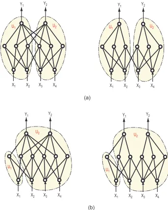
Consider different decompositions of two different networks, one in the left side of Figure 2.8 and the other one in right side of Figure 2.8. In the top decompositions, intuitively the right one is more modular than the left one. However, in the bottom decompositions, the left one is more modular than the right one since they have the same U1 unit and interactions between U1 and U2, yet the

leftU2unit has stronger couplings inside than the rightU2unit. These two different decompositions

give different results on modularity, so it is necessary to compare the modularity of their maximal decompositions in order to compare the modularity of two systems.

Decompositions of a system are hierarchical. Therefore the units are organized as a hierarchy according to their relations with other units inside the model. The neural network in Figure 2.9(a), which calculatesY1andY2from the four inputsI1, I2, I3, andX4, has two level 1 units,U1andU2,

respectively realizing outputY1andY2. U1has elements of{I1, I2, H1, H2, H3, H4, O1},5andU2has

elements of{I3, I4, H5, H6, O2}. U1 can be decomposed further as two child unitsU11 andU12. For

example, unitU11has elements{I1, H1, H2}. The right tree in Figure 2.9 represents the hierarchical

relation of the different units. The lowest module is called leave modules. Formally,

Definition 4 (Leave Module) A module which has no submodules.

As discussed in Section 2.5.3, the lower bound size of modules affect the modularity of a sys-tem. It is necessary to set up a threshold for decomposition. Threshold could be the number of elements or information inside subsystems. Also, it is possible that there are some constraints on the decomposition. For example, if the networks in Figure 2.9 are trained to learn two functions, one mapping (X1, X2) toY1and the other one mapping (X3, X4) toY2, the possible decompositions

should cluster nodesX1, X2, Y1to the same set. And, similarly, to (X3, X4, Y2). Then, modularity

of a system is taking maximum over the modularity of all the following feasible decompositions.

5

(38)

(a) Y 1 Y 2 X 4 X 3 X 2 X 1 Y 1 Y 2 X 4 X 3 X 2 X 1 (b) Y 1 Y 2 X 4 X 3 X 2 X 1 Y 1 Y 2 X 4 X 3 X 2 X 1 U 2 U 1 U 2 U 1 U 2 U 1 U 2 U 1

(39)

Hidden Layer Input Layer Output Layer (a) H 4 O 1 H 1 H 3 H 2 H 6 H 5 I 3 I 2 I 1 O 2 I 4 Y 1 Y 2 X 4 X 3 X 2 X 1 U 2 U 1 U 12 U 11 U 2 U 12 U 1 U 11 S (b) Figure 2.9: Structures of neural networks.

Definition 5 (Feasible Decomposition) A feasible decomposition is a decomposition which sat-isfies all possible constraints and in which the sizes of leave modules in the hierarchical tree should be no larger than the threshold, and the sizes of their parents are larger than the threshold.

2.5.6 Comparative Nature

It is common to say “system A is more modular than B” such and such. This requires that the formally defined modularity should be comparative. Although “modular” is a very fuzzy concept, it is feasible to define measurable modularity, just like “high” and “height.”

(40)

Fitness

Smoothed Landscape Jump

Figure 2.10: Different types of landscapes.

So, modularity should be universal in the sense that modularity is a quantitative parameter of every system. The extreme cases of modularity is a completely integrative system, which has the lowest modularity, and fully decomposable systems, which have the highest modularity.

2.5.7 Definition of Modularity

In summary, modularity has the following characteristics:

1. Hierarchy. The modularity of a system is an aggregation of the modularity at different levels. 2. Globality. Modularity is a global characteristic of a system and is an integration of the

mod-ularity of its subsystems.

3. Multi-Dimensionality. Modularity is related to many different aspects such as physical struc-ture, logical strucstruc-ture, and temporal relationships.

4. Relativity: Modularity compares inter-module interaction “density” to intra-module interac-tion “density.”

5. Universality. Modularity is defined over every system.

The modularity of a modular structure (fully decomposable) can be defined as,

Definition 6 (Modularity of a Decomposed System) Modularity is an attribute describing the degree of overall relative coupling among the parts of the decomposition at different levels in different dimensions.

(41)

of a decomposition of a system asMdandC as the set of all feasible decompositions of the system. Then

Definition 7 (Modularity of a System) Modularity of a systemMmis defined as the maximum

of the modularityMd of all possible decompositionsdinC. That is,

Mm= max

d∈CMd. (2.9)

2.6 Module

Modules in a system are the outcomes of increasing modularity of the system, so modules appear in highly modular (decomposable) systems. Since the purpose of defining modules is to make some parts of a large complex system treated nearly independently and therefore easier to analyze or design the whole system, it is necessary to have interfaces to make modules nearly independent from other parts of the system. Sometimes people want to re-use them in other complex systems, which requires that the interfaces should be standardized to be interchangeable in many different environments. Combining these points, a module can be defined as:

Definition 8 (Module) A module is a unit of a system which is nearly independent of the context and interacts with other units by interfaces.

2.6.1 System Associated

The concept of module only makes sense under a specific system, i.e., modules should be associated with some system. It is not clear to say “something is a module” without contexts, and it is better to say “something is a module of some system” or “something is a product or system.” For example, considering an automobile as a system, a gearbox should be a module of the automobile system, but for manufacturers of the gearbox, they will prefer to think it as a kind of product or system. A module could become a system if it is isolated from the system.

2.6.2 Interface

Interfaces describe in detail how modules interact, how they fit together, and how they communi-cate. Specification of component interfaces could include: attachment, spatial, transfer, control and communication, environmental, ambient, and user interfaces [84].

(42)

2.6.3 Functionality

Modules are usually designed, manufactured, and tested independently. To achieve the indepen-dence, it is necessary to provide clear design requirements and well-defined physical behavior (func-tions). So, a module generally realizes one or a few of the functions of the overall function of the system.

In system synthesis, what designers are generally required to do is to create mechanisms that function as desired or design a system to perform some functions. Pahl [71] points out that it is useful to apply functions to describe and solve design problems. Functional modeling provides a direct method for understanding and representing an overall artifact function without reliance on physical structures. Otto and Wood [70] also argued that conceptualizing, defining, or understanding an artifact, product, or system in terms of function is a fundamental aspect of engineering design. At the very beginning phase of design, there is only function structure and no physical realization,6

so in order to exploit modularity and identify modules in the initial conceptual design or reverse engineering, which reduces many efforts, development time, and costs for product design [71], it is useful to decompose conceptual designs according to function structures and, therefore, later physical designs.

2.6.4 Interchangeable

It is not necessary that modules be interchangeable. Interchangeability requires that interface speci-fications of modules should be standard. If a component is just developed and is new to the industry, then its interfaces are bound to be ill-designed and specified, and even if the component is unique to a company, then its interface specifications are generally not standardized within the industry. Only when specifications of a component become well specified and standardized do they become a standard component.

2.7 Summary

As pointed out in Chapter 1, modularity or modular structures are commonly existing in com-plex natural and artificial systems. This implies that modular structures are advantageous to non-modular structures for complex systems. This chapter begins with a discussion on the benefits of modularity, but modularity is not free, and it also has costs.

Based on the surveys on existing views on modularity, several questions about modularity have been clarified. Specifically they are system vs. model, specific meanings of “inter-module” and

6

(43)

“intra-module,” relativity of couplings, aggregation of modularity at different levels in a hierarchical structure, application domain of definition, and how to quantify couplings. Except for coupling quantification, the other 5 questions have been discussed in this chapter. The remaining question on coupling quantification will be discussed in the next two chapters.

For a nearly-decomposable system (or decomposition), modularity describes the degree of over-all relative couplings between parts at different scales in different dimensions. For a not-fully-decomposable system, modularity is defined as the maximal modularity of all feasible decompositions of the system.

(44)

Chapter 3 Quantifying Couplings with Information-Theoretic

Methods

3.1 Introduction

There are many qualitative and exploratory studies on modularity [3, 28, 46, 61, 81, 85, 86, 100], but few are quantitative [48, 29, 63]. Existing modular product design methods can be classified into the following two categories: function-based methods [71, 94] and matrix-based methods [19, 91, 27, 29, 113, 89]. Pahl and Beitz [71] developed a formal function model and proposed that modular product architectures can be derived from function diagrams which describe the flow of energy, materials, and signals between subsystems. Based on formal function models described by Pahl and Beitz, Stone et al.[94] developed a set of three heuristic methods for identifying modules from the function models. Most function-based methods are heuristic, and not quantitative, methods. The design structure matrix (DSM) representation method was invented by Donald Steward [93] and extended and refined by Steven Eppinger [19]. Most matrix-based modular product design methods are based on some quantitative measures of modularity. Most of those quantitative modularity measures typically use linkage counting methods, which compare the average number of linkages between modules with the average number of linkages inside modules. For example, following is one typical modularity measure of a product [34]:

Modularity =

PM

k=1

µPmk

i=_nk

Pmk

j=_nkRij

(mk−nk+1)2 −

Pmk

i=_nk(

Pnk−1

j=1 Rij+PNj=_mk+1Rij)

(mk−nk+1)(N−mk+nk−1)

¶

M ,

wherenk andmk are indices of the first and last component inkthmodule,M is the total number of modules inside the product,N is the total number of components in the product, andRij is the value ofith_{row and}_jth_{column element in the modularity matrix.}

(45)

design processes need some intuition and an art sense, those quantifications could be done formally in redesign processes and later phases of design processes. According to the author’s knowledge, there is no such quantitative way to quantify the interactions.

From information-theoretic views, this chapter develops mutual information-based methods which have been used to quantify independence in independent component analysis [49] to provide quan-titative ways to measure interactions. Now that information-theoretic methods can quantify in-teractions, they can directly quantify modularity without mapping designs or products to DSM or function diagrams first. Most information theoretic concepts, such as entropy and mutual infor-mation, are based on uncertainty and randomness very commonly existing in engineering practice and products, which can be modeled as stochastic systems since working conditions for engineering products are stochastic, noises in working environments are random, and the inputs of the system are random.

Since mutual information-based methods are based on randomness, systems of random variables are considered firstly, and a framework of modularity measure based on mutual information is established. Under the framework, modularity of dynamic behaviors of stochastic systems and design processes are discussed. According to information-theoretic views, adjacency matrices of weighted graphs can be mapped to covariance matrices of gaussian random variables, and it can be shown that general linkage counting methods are a special case of the information-theoretic views.

3.2 Preliminary on Information Theory

Most material in this section is from “The Theory of Information and Coding” by R. J. McEliece [62] and “Elements of Information Theory” by T. M. Cover and J. A. Thomas [15]. You can refer to these two books for more details.

3.2.1 Discrete Random Variables

The entropyH(X) of a discrete random variableX with probability distributionp(x) is defined by

H(X) =−X

x

p(x) logp(x). (3.1)

The joint entropyH(X, Y) of two discrete random variablesX andY with joint probability distri-butionp(x, y) is

H(X, Y) =−X

x,y

Information-theoretic methods for modularity in engineering design