An automated sleep-state classification algorithm for quantifying sleep timing and sleep-dependent dynamics of electroencephalographic and cerebral metabolic parameters

(1)

Nature and Science of Sleep

Dove

press

O r i g i N a l r e S e a r c h

open access to scientific and medical research

Open access Full Text article

An automated sleep-state classification algorithm

for quantifying sleep timing and sleep-dependent

dynamics of electroencephalographic and cerebral

metabolic parameters

Michael J Rempe1,2

William C Clegern2

Jonathan P Wisor2

1_{Mathematics and Computer Science,}

Whitworth University, Spokane, WA, USA; 2_{College of Medical Sciences} and Sleep and Performance Research Center, Washington State University, Spokane, WA, USA

Correspondence: Michael J Rempe Mathematics and Computer Science, Whitworth University, 300 W Hawthorne Road, Spokane, WA, 99251, USA

email [email protected]

Introduction: Rodent sleep research uses electroencephalography (EEG) and electromyography

(EMG) to determine the sleep state of an animal at any given time. EEG and EMG signals, typically sampled at .100 Hz, are segmented arbitrarily into epochs of equal duration ( usually 2–10 seconds), and each epoch is scored as wake, slow-wave sleep (SWS), or rapid-eye- movement sleep (REMS), on the basis of visual inspection. Automated state scoring can minimize the burden associated with state and thereby facilitate the use of shorter epoch durations.

Methods: We developed a semiautomated state-scoring procedure that uses a combination of

principal component analysis and naïve Bayes classification, with the EEG and EMG as inputs. We validated this algorithm against human-scored sleep-state scoring of data from C57BL/6J and BALB/CJ mice. We then applied a general homeostatic model to characterize the state-dependent dynamics of sleep slow-wave activity and cerebral glycolytic ﬂux, measured as lactate concentration.

Results: More than 89% of epochs scored as wake or SWS by the human were scored as the

same state by the machine, whether scoring in 2-second or 10-second epochs. The majority of epochs scored as REMS by the human were also scored as REMS by the machine. However, of epochs scored as REMS by the human, more than 10% were scored as SWS by the machine and 18 (10-second epochs) to 28% (2-second epochs) were scored as wake. These biases were not strain-specific, as strain differences in sleep-state timing relative to the light/dark cycle, EEG power spectral profiles, and the homeostatic dynamics of both slow waves and lactate were detected equally effectively with the automated method or the manual scoring method. Error associated with mathematical modeling of temporal dynamics of both EEG slow-wave activity and cerebral lactate either did not differ significantly when state scoring was done with auto-mated versus visual scoring, or was reduced with autoauto-mated state scoring relative to manual classification.

Conclusions: Machine scoring is as effective as human scoring in detecting experimental

effects in rodent sleep studies. Automated scoring is an efficient alternative to visual inspection in studies of strain differences in sleep and the temporal dynamics of sleep-related physiologi-cal parameters.

Keywords: EEG, automated scoring, principal component analysis, Bayes classification

Introduction

In rodent polysomnographic studies, electroencephalographic (EEG) and electromyo-graphic (EMG) data are recorded at a high sampling rate, typically 100 Hz or more, and then segmented into epochs of arbitrary duration (typically 2–10 seconds in rodents),

Nature and Science of Sleep downloaded from https://www.dovepress.com/ by 118.70.13.36 on 24-Aug-2020

For personal use only.

Number of times this article has been viewed

This article was published in the following Dove Press journal: Nature and Science of Sleep

(2)

Dovepress rempe et al

each of which is classified as wake, slow-wave sleep (SWS), or rapid-eye-movement sleep (REMS) on the basis of visual inspection. Although this approach is the gold standard for state scoring, there are several drawbacks: states determined by manual scoring can vary from person to person; when EEG and EMG features ﬂuctuate within a given epoch, the user must assign a single state; and the process is labor intensive and time consuming.

Automated scoring algorithms have been used as an alter-native to manual state scoring. Among previously proposed automated scoring approaches are: computing a quantitative state index for each epoch and scoring based on these indices1

using principal component analysis (PCA) and manual clus-tering of epochs in PCA space;2_{using a naïve Bayes classifier;}3

using linear discriminant analysis;4_{using classification trees;}4,5

using a support vector machine;6_{using a fully unsupervised}

Bayesian classifier;7_{and several methods that use a single}

channel of EEG data to categorize human sleep.8–10_{Here we}

present a hybrid approach to automated scoring of rodent sleep EEG and EMG data in which human-scored epochs are used as a training template for automated state scoring. We combine the PCA approach of Gilmour et al2_{with a naïve}

Bayes classifier that uses the first three principal-component vectors as inputs. Our method is therefore similar to that of Rytkönen et al,3_{except that we employ the naïve Bayes}

clas-sifier on the data after constructing manual scoring-derived, state-specific feature vectors and keeping only the first three principal component vectors, rather than splitting up the data into logarithmic frequency bands.

When sleep is scored in epochs, epoch duration is, to an extent, arbitrary. The duration of epochs used often depends on the duration of the sleep-related phenomena of interest in a given study. For instance, in studying brief REMS-related eye movements, 2-second epochs have been used.11_{In studying}

state-switching instability at sleep onset, 4-second epochs have been used when longer epoch durations failed to reveal this instability.12_{In studying EEG changes across}

SWS-to-REMS transition, a process that evolves gradually over 1–2 minutes, 10-second epochs were used to demonstrate that dynamic.13_{In studying the gross disruption of sleep/}

wake cycles by maternal separation of rodents, 30-second epochs were used.14_{These examples illustrate that sleep must}

be studied on different time scales and that machine scoring needs to be validated for these different time scales.

When choosing epoch duration, one balances countervail-ing factors. The fidelity of state scorcountervail-ing is increased as epoch duration is shortened, as the probability of a state transition occurring within each epoch is thereby reduced. However, the

effort associated with state scoring by visual inspection is increased as epoch duration is shortened. Because different research groups use different epoch lengths, it can be dif-ficult to compare sleep data across studies. This issue arises when epoched data has been used in mathematical modeling of sleep-dependent slow-wave dynamics,15–18_{as the time}

constants that describe temporal dynamics may be a function of epoch duration.

Here we present a systematic investigation of the effect of epoch length on sleep-dependent dynamics of slow-wave activity (SWA) and lactate concentration in the cerebral cortex. The latter serves as a marker for glucose utilization and varies as a function of sleep state.19–21_{To investigate the effect of}

epoch length on these dynamics, we segmented datasets into both 10-second and 2-second epochs. We used the hybrid PCA/ Bayes classifier to automatically score the recordings.

The agreement of a novel automated scoring method with scoring of data by an investigator is a typical performance measure for the novel method. But to the extent that the purpose of scoring sleep is to identify experimental effects of independent variables on dependent variables, whether or not the algorithm detects the same experimental effects as the human scorer is an important consideration as well. Therefore, the algorithm is applied here in two strains of mice and across the entire circadian cycle, in order to deter-mine whether time-of-day effects and differences between the strains in time spent asleep measured by human scoring are also detected algorithmically. Likewise, mathematical modeling with human-scored sleep-state data as an input parameter predicts the dynamics of SWA and lactate concen-tration over time.22_{Whether sleep-state data from automated}

scoring can effectively serve as a predictive parameter for modeling physiological processes is yet another consider-ation in evaluating a novel autoscoring algorithm.

Our goals for the current study were thus: 1) to deter-mine the agreement between a combined PCA/naïve Bayes autoscoring method and human scoring in measuring sleep timing and sleep homeostatic dynamics; 2) to determine the relative effectiveness of the autoscored and human-scored datasets in detecting experimental effects; and 3) to use this efficient autoscoring approach to determine the effect of 2-second versus 10-second epoch length on the time dynam-ics of EEG SWA and lactate concentration.

Methods

Experimental subjects

All procedures adhered to National Research Council guide-lines (Institute of Laboratory Animal Resources NRC 1996)

(3)

Dovepress Automated quantification of sleep-dependent parameters

and were approved by the institutional animal care and use committee of Washington State University. Male mice of the C57BL/6J (B6, n=12) and BALB/CJ (BA, n=10) strains were used in these experiments. They were purchased at age 8 weeks from Jackson Laboratories (Bar Harbor, ME, USA; strains #664 and #651). Animals were housed in a light/dark 12:12 cycle with unrestricted access to standard laboratory chow and water.

Surgical preparation of subjects

Surgery was performed as described previously,21,23_under

isoﬂurane anesthesia. Mice were surgically equipped for bilateral referential frontoparietal EEGs and neck EMGs. Frontal EEG electrode locations were 1.5 mm lateral to the midline and 1 mm anterior to bregma. The parietal EEG elec-trode location was 1.5 mm left of midline and 2 mm anterior from lambda. A guide cannula for placement of a lactate biosensor20,21,23_{was placed in the left frontal cerebral cortex}

1.1 mm anterior and 1.65 mm lateral from bregma. A dummy stylet was placed in the guide cannula until the day of experi-mentation, 10–14 days after surgery. Experimentation was completed within 3 weeks of surgical implantation.

Data collection and analysis

Sleep data were scored by trained experts, as in previous work.21,24,25_{Epochs in which EMG amplitude was relatively}

high and EEG amplitude was relatively low were scored as wake. Epochs in which EMG amplitude was relatively low and EEG amplitude relatively high were scored as SWS. Epochs in which both EMG amplitude and EEG amplitude were low and in which theta (5–9 Hz) activity predominated in the EEG were scored as REMS. Scoring of REMS was additionally context-dependent, in that epochs meeting these criteria that occurred within wake episodes were scored as wake, not REMS.

Lactate was measured using a lactate oxidase based bio-sensor implanted in the frontal cerebral cortex, as described elsewhere.20,21,23_{This technique was first published in 1997}26

and has since been refined and commercialized by Pinnacle Technology, Inc. (Lawrence, KS, USA; part #7004-Lactate). The sensing mechanism consists of a platinum–iridium electrode surrounded by a layer of lactate oxidase molecules. Metabolism of lactate by lactate oxidase produces hydro-gen peroxide, which produces a current in the platinum– iridium electrode. The current at the sensing electrode is proportionate to the concentration of the substrate for the lactate oxidase enzyme (lactate, the product of glycolysis). Current is monitored at a sampling rate of 1 Hz, providing

a moment-by-moment estimate of lactate concentration in the cerebral cortex. Current was averaged across all values within each epoch of data analyzed (n=10 for 10-second epochs; n=2 for 2-second epochs). In order to eliminate noise in the signal from the sensor, each epoch’s average value was compared with the mean of the previous ten epoch values. If it deviated from that mean by more than ten standard devia-tions of that mean, the value for that epoch was replaced by the mean value.

On the day of experimentation, the lactate sensor was precalibrated, as described elsewhere.21,23_{Approximately}

8 hours into the light portion of the light/dark 12:12 cycle, the dummy stylet was removed from the guide cannula and the lactate sensor was inserted into the guide cannula. The uninsulated, enzymatically active portion of the sensor was embedded at a depth of 1 mm in the cerebral cortex. This depth targets the deeper layers of cerebral cortex, although placement was not verified histologically. The animal was placed into a cylindrical cage, where it remained throughout the duration of the recording session. EEG, EMG, and lactate biosensor current were monitored continuously at 400 Hz for 40–48 hours thereafter. Data that occurred after insertion of the lactate sensor and before the second SWS episode of 1 minute or longer was not included due to exponential decay of current from the lactate sensor in this equilibrating phase.

For comparison of the effectiveness of human scoring and machine scoring in detecting strain differences in sleep timing across 10-second epochs, 8,640 epochs, represent-ing a complete circadian cycle, were subjected to analysis. Comparing machine scoring of 10-second epochs to manual scoring in this time range allowed us to determine whether there was a circadian phase-specific bias in the performance of the algorithm. To assess machine-scoring performance relative to human performance in scoring 2-second epochs, we sought to perform analysis on a similar number of epochs as in the 10-second epoch dataset. Each of the epochs used for validation of the algorithm had to be scored by a human, and we anticipated that scoring the numbers of 2-second epochs in one circadian cycle (43,200 epochs) would pro-duce significant fatigue in the human scoring the file. This fatigue would decrease the accuracy of the human scoring and thereby confound any measurement of the machine scoring accuracy for 2-second epochs relative to 10-second epochs. Instead, we reasoned that 8,640 2-second epochs represent 4.8 hours, so we added an additional 360 epochs to make the dataset an even 5 hours. Data from the 5-hour interval between 10 am and 3 pm were used in this analysis because at that time of day rodents transition across all three

(4)

states most reliably, allowing for a thorough assessment of the accuracy of scoring across all three states.

PCA and machine learning

To autoscore sleep data consisting of EEG and EMG data binned into 2-second or 10-second intervals, we used a com-bination of PCA and machine learning. The PCA began by constructing seven “feature” vectors from the EEG and EMG data traces, following Gilmour et al.2_{The seven features are:}

1) EEG power in the 1–4 Hz (delta) range; 2) EEG power in the 5–9 Hz (theta) range; 3) EEG power in the 10–20 Hz (low beta) range; 4) EEG power in the 30–40 Hz (high beta) range; 5) EMG power; 6) theta-to-delta ratio; and 7) beta-to-delta ratio. Each vector contained one element for each epoch in the recording, so each epoch can be thought of as a point in a seven-dimension space. PCA transforms these seven vectors into a set of seven linearly uncorrelated vectors called principal components. The first principal component points in the direction (in seven-dimension space) of great-est variance in the data, and each succeeding component points in the direction of greatest variance with the restric-tion that it is orthogonal to each of the preceding principal components.

This idea can be visualized in the following manner: because each epoch of data is given a value in seven different categories, it can be visualized as a point in seven-dimension space. If every epoch in a recording is plotted in this seven dimension space, they may form a random cloud of data with no discernible pattern. However, more commonly, when plotted this way the data tend to line up along one or two directions that are not parallel to any of the coordinate axes. The directions along which they line up are the principal components. It is important to note that the principal com-ponents are different for each recording, as each one requires a different combination of the seven features to best explain the variation in the data.

Once the principal component vectors were found for the data, we computed the percentage of the total variance in the feature vectors that was explained by each principal component. For every dataset included in this study, the first three principal component vectors accounted for more than 99% of the variance in the feature vectors, so we reduced the seven-dimension feature space down to three by keeping only the first three principal components. Once this transformation was made, the data were plotted with respect to the first three principal components, and clustering of epochs into wake, non-REM sleep (NREMS), and REMS was clearly visible for each dataset. Moreover, plotting the data using only the first

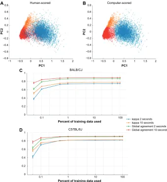
two principal component directions yielded distinct clusters (Figure 1A), indicating that PCA was effectively separating out the sleep states.

We combined this principal component approach with a naïve Bayes classifier to automatically score files. A naïve Bayes classifier requires that a subset of the epochs be scored by a human in order to train the classifier to score the rest of the epochs. The naïve Bayes classifier uses the training data to divide the three-dimensional principal component space into three distinct zones, one for each sleep state. Each unscored epoch is then scored on the basis of which zone it falls into. Finally, as REMS is consistently preceded by non-REMS rather than by wake in wild-type rodents, epochs scored as REMS that were preceded by at least 30-seconds of wake were rescored as wake. See the Discussion for more details. We implemented both the PCA and the naïve Bayes scor-ing in MATLAB. Scripts are available to interested parties on request. We first applied the PCA/naïve Bayes hybrid approach to fully-scored 24-hour 10-second epoch data files using the data from 10 am to 2 pm (Zeitgeber time 4–8; a time when all three states alternate on a regular basis) as training for the Bayes scoring algorithm. We used a variety of agreement statistics to compare the scores determined by the algorithm to those made by a human (see Agreement statistics, below). Plotting the machine-scored data along the first two principal component directions yielded images similar to the human-scored data (Figure 1B).

Agreement statistics

To quantify the agreement of the machine scoring and the human scoring, we calculated five statistical measures. Global agreement is the percentage of total epochs that are scored the same by the human and the algorithm. We also calculated the percentage agreement for wake by counting the number of epochs scored as wake by both human and machine, and divided by the number of epochs scored as wake by the human score. We repeated this calculation for SWS and REMS. Finally, we computed Cohen’s unweighted kappa,27_{a way}

to quantify agreement while accounting for agreement that would happen due to chance alone.

To determine how many human-scored epochs were needed to successfully train the algorithm to score an entire dataset, we ran the autoscoring procedure using various percentages of the human-scored data as training templates (Figure 1C and D). For each percentage, we randomly selected the appropriate number of human-scored epochs, while ensuring that in each case at least one epoch of each sleep state was present. For both strains, with data binned in

(5)

10-second epochs the kappa statistic and the global agreement approached 90%, using only about 1% of the human-scored dataset for training. For each run of the autoscoring algo-rithm, we used 4 hours of human-scored data as training. This corresponds to 9% of a 43-hour recording (as in Figure 1A and B), 16% of a 24-hour recording using 10-second epochs, and 80% of 8,640 2-second epochs.

Mathematical models of delta

activity and lactate dynamics

We employed a general homeostatic model to quantify the temporal dynamics of both EEG and lactate concentration.22,28

To model SWA (the EEG power in the 1–4 Hz range, called Process S) we assumed that S increases exponentially toward a constant upper asymptote (UA) during wake and REMS, and decreases exponentially toward a constant lower asymp-tote (LA) during SWS. The time course of S can be found by solving the following differential equation:

dS

dt = S LA S UA

−  



 − + −

−  



 −

σ

τ σ τ

1

1 1

d i

( ) ( ) ( ) (1)

where τi and τd are the time constants of the increasing and

decreasing exponential functions, respectively, and where 0.8

BALB/CJ Human-scored

C57BL/6J

Computer-scored

C

D

B A

0.6

0.4

0.2

0

0.8

0.6

0.4

0.2

0

0.8 1 1

0.6

0.4

0.2

0 −0.2

−0.4

−0.6

−0.8

0.8

0.6

0.4

0.2

0

−0.2

−0.4

−0.6

−0.8

−1 −0.5 0 0.5

PC1

Percent of training data used

PC1

PC

2

PC

2

1 1.5 2 −1 −0.5 0 0.5

0.1 1 10 100 _{kappa 2 seconds}

kappa 10 seconds Global agreement 2 seconds Global agreement 10 seconds

0.1 1 10 100

1 1.5 2

Figure 1 Comparison of human scoring to machine scoring.

Notes: Principal component plots of a 43-hour recording scored in 10-second epochs by a human (A) and using the machine learning algorithm (B). Each dot represents one 10-second epoch, and its color represents sleep state (SWS = blue, wake = red, reMS = orange). The computer-scored plot used data from 10 am to 2 pm (Zeitgeber time 4–8 in the first complete light/dark cycle of the recording) as training data to score every epoch in the entire 43-hour recording. Both for BALB/CJ mice (C) and C57BL/6J mice (D), the agreement between machine-scored and human-scored increased as more of the training data were used. For each genetic strain, 8,640 2-second epochs and 8,640 10-second epochs were scored by a human and by the autoscoring procedure, with 0.05%, 0.1%, 0.5%, 1%, 10%, 50%, 80%, and 100% of those 8,640 epochs used as training data. These correspond to 4 epochs, 9 epochs, 43 epochs, 86 epochs, 864 epochs, 4,320 epochs, 6,912 epochs, and 8,640 epochs, respectively. In each case it was ensured that at least one epoch of each state was present. Two measures of agreement between the human scoring and the machine scoring were computed: Cohen’s kappa and global agreement. The x-axis shows the percentage of the 8,640 epochs used as training data, indicating that the learning algorithm requires only about 1% of the training data to reach optimal performance.

Abbreviations: REMS, rapid-eye-movement sleep; SWS, slow-wave sleep.

(6)

σ=1 during an epoch scored as SWS and σ=0 otherwise. The model for the wake–sleep temporal dynamics of lactate (which we term Process L) is identical to that of Process S, except that UA and LA, respectively, are functions of time rather than constants. The equation is as follows:

dL

dt = L LA t L UA t

−  



 − + −

−  



 −

σ

τ σ τ

1

1 1

d i

( ( )) ( ) ( ( )) (2)

LA and UA were made functions of time to account for the changes in the lactate signal due to the gradual decay in the output of the lactate sensor over the course of the recording.22

To compute UA(t) and LA(t), we constructed a histogram of the lactate signal in a 2-hour moving window throughout the entire recording. The 90% level of these histograms was chosen as UA and the 10% level was chosen as LA. For both the Process S and Process L models the time constants for the rates of increase (τi) and decrease (τd) were optimized,

via the Nelder–Mead/simplex method, to minimize the error of the model relative to the raw data.29

Results

Sleep state scoring: human

versus machine

Visual inspection of the machine scoring compared with the human scoring (based on EEG and EMG signals) showed a high degree of agreement (Figure 2). To quantify agreement between the two scoring methods, we computed Cohen’s kappa, as well as global agreement and agreement of each of the states (Figure 3). Global agreement and kappa were high for both strains and both epoch lengths. We also pooled the 10-second epoch data and the 2-second epoch data from both strains, and we constructed confusion matrices for each (Table 1) indicating agreement between human scoring and the machine algorithm for each state.

The percentage of correct classifications for each state appears in the entries along the diagonal of the matrix, and misclassifications appear in the off-diagonal entries. For example, the first data row of Table 1 indicates that of all epochs scored as wake by the human scorer, 89.54% of those were also scored as wake by the algorithm, 9.71% of those epochs were scored as SWS, and 0.75% were scored as REMS.

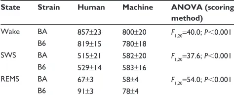
When data were processed in 10-second epochs, the scor-ing algorithm scored more epochs as SWS than did human scoring (Table 2; F_1,20=37.6; P,0.001; main effect of scoring method), at the expense of both REMS (F_1,20=54.0; P,0.001; main effect of scoring method) and wake (F_1,20=40.0;

P,0.001; main effect of scoring method). The absence of a significant time × scoring method interaction (F_23,920=1,

P.0.05) for any of the three states indicates that there was not a time-of-day–specific bias in the disagreement between scoring methods. Of epochs scored as wake by a human, 10% in BA and 10% in B6 were not scored as wake by machine. The human versus machine scoring discrepancy resulted in a 5% (B6 mice) to 7% (BA mice) reduction in total wake time over 24 hours with machine scoring relative to human scoring (Figure 4A and B; main effect of scoring method, F_1,20=40.0;

P,0.001). Of epochs scored as REMS by a human, 33% in

BA and 25% in B6 were not scored as REMS by machine. Consequently, the number of epochs scored as REMS over 24 hours was reduced by 13% (BA mice) to 14% (B6 mice; Figure 4E and F; main effect of scoring method, F_1,20=37.6;

P,0.001). Epochs scored as either of the two desynchronized states by human scoring were more likely to be scored as SWS by machine. Thus, the number of epochs scored as SWS by machine exceeded that of human scoring by 10% in BA and 13% in B6 (Figure 4C and D; main effect of scoring method,

F_1,20=54.0; P,0.001). Bias in the machine scoring was not strain-specific, as strain × scoring method interaction was not significant for any of the three states (F_1,20=1.6; P.0.2).

02:00 am EMG

(mv) EEG (µv)

300 200 100

−100 −200 −300

−0.2 0.0 0.2 0.4

−0.4 0

Human autoscored

02:20 am 02:40 am 03:00 am 03:20 am 03:40 am

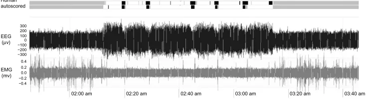
Figure 2 EEG and EMG data for comparison of human scoring and machine scoring.

Notes: The top two traces show human and autoscored sleep states for each 10-second epoch of the EEG and EMG shown in the lower panels. The sleep states are labeled with color (gray for wake, white for SWS, and black for REMS).

Abbreviations: EEG, electroencephalography; EMG, electromyography; REMS, rapid-eye-movement sleep; SWS, slow-wave sleep.

(7)

Table 1 Confusion matrix, human versus machine scoring;

per-centage of correct classifications

Wake (machine)

SWS (machine)

REMS (machine) Ten-second epochs

Wake (human) 89.54 9.71 0.75

SWS (human) 3.31 95.58 1.11

REMS (human) 18.66 10.89 70.45

Two-second epochs

Wake (human) 92.03 7.29 0.68

SWS (human) 6.98 91.48 1.54

REMS (human) 28.12 14.95 56.93

Abbreviations: REMS, rapid-eye-movement sleep; SWS, slow-wave sleep.

Table 2 Sleep states in 10-second epochs, human versus machine

scoring (minutes/24 hours)

State Strain Human Machine ANOVA (scoring

method)

Wake BA 857±23 800±20 F_1,20=40.0; P,0.001

B6 819±15 780±18

SWS BA 515±21 582±20 F_1,20=37.6; P,0.001

B6 529±14 583±16

reMS BA 67±3 58±4 F_1,20=54.0; P,0.001

B6 91±3 78±4

Abbreviations: ANOVA, analysis of variance; BA, BALB/CJ mice; B6, C57BL/6J mice; REMS, rapid-eye-movement sleep; SWS, slow-wave sleep.

1

0.9

0.8

0.7

0.6

0.5

0.4

0.3

0.1 0.2

0

BA 10-second B6 10-second

Agreement metric

BA 2-second B6 2-second

Wake SWS REMS Global kappa

Figure 3 Agreement statistics between human scoring and machine scoring.

Notes: For the data scored in 10-second epochs, the agreement statistics compare the human and machine scoring for the entire 40–48-hour recording. For the data in 2-second epochs, the comparison is between 8,640 epochs that were scored by hand and the same 8,640 epochs scored by the automated scoring algorithm. Lines inside boxes represent median values. The lower end of each box indicates the first quartile of the data (Q1), and the upper end represents the third quartile (Q3). To draw the whiskers, we calculated the interquartile range (IQR), which is the distance between Q1 and Q3. The lower whisker indicates the lowest data point within 1.5 IQR of Q1. The upper whisker indicates the largest data point within 1.5 IQR of Q3. Outliers more than 1.5 IQR but less than 3 IQR above Q3 or below Q1 are represented with open circles.

Abbreviations: B6, C57BL/6J mice; BA, BALB/CJ mice; REMS, rapid-eye-movement sleep; SWS, slow-wave sleep.

When data were scored in 2-second epochs, SWS as a percentage of time was no longer significantly affected by scoring method (F_1,20=3.3; P=0.086; Figure 5C and D). However, machine scoring systematically overrepresented wake (F_1,20=262.4; P,0.001; Figure 5A and B) and under-represented REMS (F_1,40=198.2; P,0.001; Figure 5E and F) relative to human scoring.

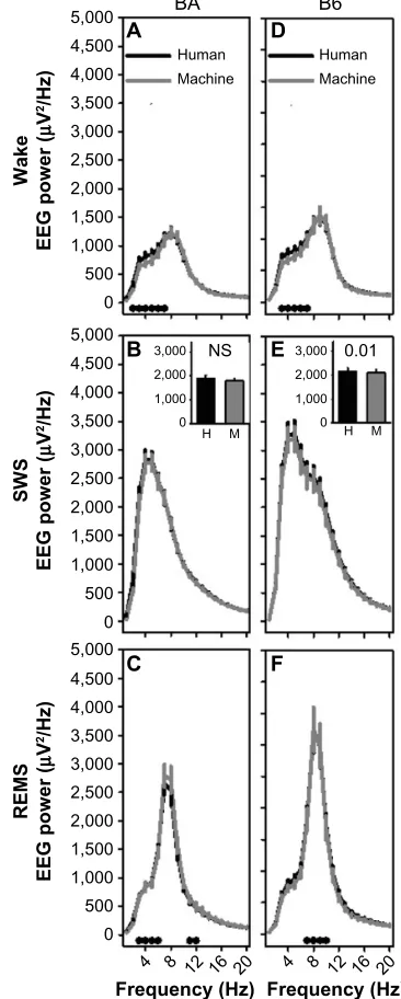
EEG power spectra: human

versus machine

EEG power spectra exhibited the typical state dependence irrespective of state-scoring method and epoch duration (Figure 6). In both strains, slow (,6 Hz) activity pre-dominated in SWS; theta (6–8 Hz) activity prepre-dominated in REMS; EEG amplitude remained relatively low at these frequencies in wake. Although the EEG spectral power curve for machine-scored states largely obscured that of human-scored states in both strains, there were significant

scoring method × frequency interactions for wake (10-second

F_19,380=10.1, P,0.001; 2-second F_19,380=4.0, P,0.001) and REMS (10-second F_19,380=3.7, P,0.001; 2-second F_19,380=2.2,

P=0.003), but not SWS. Additionally, 1–4 Hz SWA was reduced modestly (2%) but significantly in machine-scored 10-second epochs of SWS relative to human-scored SWS within the B6 strain specifically (Figure 6E, inset).

Measuring sleep state-dependent

dynamics of SWa and lactate:

human versus machine

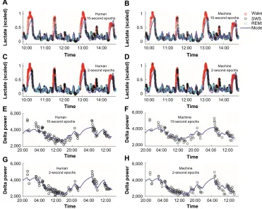
To further investigate the utility of the machine scoring, we employed a homeostatic model to predict the state-dependent dynamics of SWA and cerebral lactate concentration.22_We

applied this model to both the human-scored and machine-scored data using 10-second epochs and 2-second epochs (Figure 7). The temporal dynamics of the optimized model were unchanged with respect to scoring method using both

(8)

80 BA

Wake (%)

SWS (%)

REMS (%

)

B6

60

Human Machine

60 40

40 20

20 0

0

Clock time Clock time

F E

C

B A

D

20 0 4 8 12 16 20 20 0 4 8 12 16 20 4

8

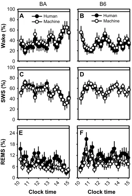
Figure 4 Sleep-state percentages in human-scored versus machine-scored 10-second epoch data.

Notes: Data from the BA strain (left column) and the B6 strain (right column), were binned into 60-minute intervals. Graphs represent the percentage of each interval spent in wake (A and B), SWS (C and D), and REMS (E and F). Open circles

represent machine-scored data and filled circles represent human-scored data. Dark and light phases are indicated by black and white bands at the top of each panel.

80

100 BA

Wake (%)

SWS (%)

REMS (%)

B6

60

Human Machine

40

20

0

80 100

60

40

20

0

24

18

12

6

0

F E

C

B A

D

10 11 12 13 14 15 10 11 12 13 14 15

Figure 5 Sleep-state percentages in human-scored versus machine-scored 2-second epoch data.

Notes: Data from the BA strain (left column) and the B6 strain (right column) were binned into 12-minute intervals. Graphs represent the percentage of each interval spent in wake (A and B), SWS (C and D), and REMS (E and F). Open circles

represent machine-scored data and filled circles represent human-scored data. Data are from Zeitgeber time 4–9.

10-second epochs (Figure 7A, B, E, and F) or 2-second epochs (Figure 7C, D, G, and H). Because only 8,640 of the 2-second epochs were scored by a human, only those data are shown in panels 7A–7D. This corresponds to 4.8 hours of data starting at 10 am. The dynamics of the lactate signal were minimally affected by the choice of 2-second or 10-second epoch length. In panels 7E–7H, the homeostatic model was fit to delta power (1–4 Hz) in 5-minute episodes made up of at least 90% SWS. Although the model of delta power also used 8,640 epochs as training for the machine scoring, all of the data are shown since the temporal dynamics of SWA are slower than those of lactate.

In modeling sleep-state SWA dynamics there was a sig-nificant effect of scoring method on both τi (the optimized

time constant for the rise of SWA as a function of prior time spent in desynchronized states; Figure 8A and C) and τd

values (the optimized time constant for the decline of SWA as a function of prior time spent in SWS; Figure 8B and D)

in modeling sleep-state SWA dynamics. Both time constants optimized at higher values in the machine-scored datasets relative to the human-scored datasets, irrespective of strain (strain × scoring method interaction, F_1,20,0.2, P.0.60; see strain differences discussed below). In modeling SWA in 10-second epochs, the mean optimized τi values (3.2 hours)

and τd (3.8 hours) across all animals from machine-scored

data were greater than those generated from human-scored data (2.6 hours, 3.5 hours) by 10% and 21%, respectively. In modeling SWA in 2-second epochs, the mean optimized

τi values (4.8 hours) and τd (3.8 hours) across all animals

from machine-scored data were greater than those gener-ated from human-scored data (4.2 hours, 3.1 hours) by 12% and 25%, respectively. Scoring method significantly affected τd (Figure 8F) but not τi values (Figure 8E) for the

temporal dynamics of lactate concentration in 10-second epochs. In modeling lactate in 10-second epochs, the mean optimized τd values (0.23 hours) across all animals from

(9)

Residuals (Figure 9), a measure of the deviation of optimized mathematical modeling values from the data being modeled, provide an indication of the performance of the model. Lower residuals indicate a better fit to the data being modeled. Two-way analysis of variance with strain as a between-subjects variable and scoring method (auto-mated versus manual) as a within-subjects variable indicated significant effects of scoring method on residual values for modeling lactate dynamics in 10-second epochs (Figure 9C;

F_1,20=5.3, P=0.032) and SWA dynamics in 2-second epochs (Figure 9B; F_1,20=5.3, P=0.032). Scoring method did not significantly affect residuals for lactate dynamics in 2-second epochs (Figure 9D) or SWA dynamics in 10-second epochs (Figure 9A). Residuals did not vary as a function of strain in any of the four analyses, nor were scoring method × strain interactions significant. Where residuals were affected by scoring method (Figure 9B and C), the residuals were lower (albeit modestly) for automated scoring than for manual scoring. Thus, the performance of automated scoring is as effective as, if not modestly more effective than, manual scoring, for use in modeling sleep state-dependent dynamics of physiological variables.

Machine scoring detects strain

differences in sleep timing, EEG

power spectra, and sleep-dependent

physiological parameter dynamics

Strain × scoring method interaction was not significant for any of the three states as a percentage of time, which indicates that there was not a strain-specific bias in the disagreement between scoring methods. The BA and B6 strains, by virtue of genomic differences, exhibit differences in sleep-state timing. Both human and machine scoring detected a significant main effect of strain on REMS as a percentage of time across the entire 24-hour light/dark 12:12 cycle (Table 3). Neither wake as a percentage of 24 hours nor SWS as a percentage of 24 hours differed between the two strains regardless of state-scoring method; however, all three states exhibited time-of-day–specific strain effects regard-less of whether states were scored by human or machine, as indicated by significant strain × time interaction for both scoring methods (Table 3).

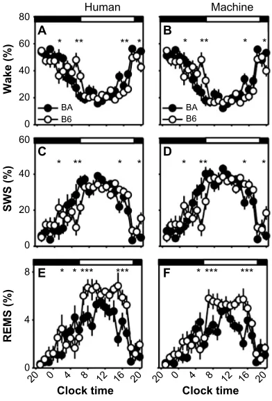
Posthoc comparisons across strains yielded strikingly similar time-of-day–specific effects of strain on sleep timing in the human-scored and machine-scored datasets (Figure 10). For instance, SWS as a percentage of time dif-fered significantly between strains (Fisher’s protected least-significant difference) in hours 5, 9, 10, 19, and 24, and at

5,000 A

B

C F

D

E

BA B6

4,500 4,000 3,500

Human Machine

2,500 3,000

2,000 1,500 1,000 500 0 5,000

3,000 2,000 1,000 0

H M H M

0.01 4,500 NS

4,000 3,500

2,500 3,000

2,000 1,500 1,000 500 0 5,000 4,500 4,000 3,500

2,500 3,000

2,000 1,500 1,000 500 0

Frequency (Hz)

REMS

EEG power

(

µ

V

2/Hz)

SWS

EEG power

(

µ

V

2/Hz)

Wake

EEG power

(

µ

V

2/Hz)

Frequency (Hz)

4 8 12 16 20 4 8 12 16 20

Figure 6 Machine-scored data in 10-second epochs exhibit similar frequency profiles to human-scored data.

Notes: The left column shows data for the BA strain and the right column shows data for the B6 strain. For wake (A and D), SWS (B and E), and REMS (C and F), the frequency profiles of the human-scored data (black line) and those of the machine-scored data (gray line) are shown. The black dots in panels (A, C, D and F) indicate

frequency bands in which posthoc comparisons (Fisher’s protected least-significant difference) indicated a difference between the curves. The insets in panels (B and E)

show 1–4 Hz SWA. P-values in these insets indicate main effect of scoring method on SWa.

Abbreviations: B6, C57BL/6J mice; BA, BALB/CJ mice; EEG, electroencephalography; EMG, electromyography; H, human; M, machine; NS, not significant; REMS, rapid-eye-movement sleep; SWA, slow-wave activity; SWS, slow-wave sleep.

machine-scored data were greater than those generated from human-scored data (0.18 hours) by 23%. Scoring method did not significantly affect either time constant, τd (Figure 8H)

or τi (Figure 8G) for the temporal dynamics of lactate

con-centration in 2-second epochs.

(10)

no other times, regardless of whether states were scored by human or machine. Wake time differed significantly between strains in hours 5, 9, 10, 19, and 24, regardless of whether states were scored by human or machine. REMS time differed significantly between strains in hours 9, 11–13, and 19–21 of recording, regardless of whether states were scored by human or machine. Thus, although machine-based scoring exhibited a significant bias toward SWS, it nonetheless detected the experimental effect of strain on sleep timing. This analysis was not repeated for the 2-second epoch data, as those 8,640 epochs represented a 5-hour window within which daily rhythms of sleep and wake are not apparent.

Repeated-measures analysis of variance indicated signifi-cant strain × frequency interactions affecting spectral profiles of wake, SWS, and REMS in both human-scored and machine-scored datasets for both 10-second (Table 4) and 2-second epoch data (not shown). Posthoc comparisons of EEG spec-tral profiles between strains across 1 Hz bins indicated that the strain difference detected in the EEG spectral profile in human scored datasets was replicated in the machine-scored

datasets (Figure 11). For instance, in 10-second epochs scored as wake, spectral power in the 9–11 Hz range was elevated in B6 mice relative to BA mice in both the human-scored and machine-scored datasets (Figure 11A and D). In 10-second epochs scored as SWS, spectral power in the 3–12 Hz range was elevated in B6 mice relative to BA mice in both the human-scored and machine-scored datasets (Figure 11B and E). In 10-second epochs scored as REMS, spectral power in the 6–11 Hz range was elevated in B6 mice relative to BA mice in both the human-scored and machine-scored datasets (Figure 11C and F). These data demonstrate that strain dif-ferences in EEG oscillatory activity across sleep states were detected by the machine-scoring method. Similarly, the over-lap between scoring methods in detecting strain differences in EEG spectral profiles within the 2-second datasets was near total (data not shown).

The temporal dynamics of both EEG SWA and lactate concentration across 10-second epochs were strain depen-dent regardless of scoring method (Figure 8A, B, E, and F). Strain comparison of SWA τi and τd via Student’s t-test

A

1

0.5

Lactate (scaled)

Lactate (scaled) Lactate (scaled)

Delta power

Delta power Delta power

Lactate (scaled)

0

1

0.5

0

1

0.5

0 1

0.5

0

10:00 11:00 12:00

Time Time

Time

Time Time

Time

Time Time

13:00 14:00 10:00 11:00

Wake SWS REMS Model

12:00 13:00 14:00

10:00 11:00 12:00 13:00 14:00 10:00

6,000

4,000

2,000

6,000

4,000

2,000

6,000

4,000

2,000

6,000

4,000

2,000 11:00 12:00

12:00 04:00

20:00 20:00 04:00 12:00 20:00 04:00 12:00 20:00 04:00 12:00

12:00 04:00

20:00 20:00 04:00 12:00 20:00 04:00 12:00 20:00 04:00 12:00 13:00

Human 2-second epochs

Human 10-second epochs

Human

2-second epochs 2-second epochsMachine Machine 10-second epochs

Machine 2-second epochs

Machine 10-second epochs Human

10-second epochs

14:00

B

D C

E F

H G

Figure 7 Homeostatic modeling of lactate data and SWA scored by human or machine.

Notes: The left column shows human-scored data and the right-hand column shows machine-scored data. The top four panels show scaled lactate data in 10-second epochs scored by a human (A), 10-second epochs autoscored (B), 2-second epochs scored by a human (C), and 2-second epochs autoscored (D). The bottom four panels show SWA in 5-minute sleep episodes using 10-second epochs scored by a human (E), 10-second epochs autoscored (F), 2-second epochs scored by a human (G), and 2-second

epochs autoscored (H). In each panel, a homeostatic model for lactate or SWA was fit to the data (solid curve). The difference in time scale between the lower panels and the upper panels reﬂects the difference in temporal dynamics of SWA versus those of lactate.

Abbreviations: REMS, rapid-eye-movement sleep; SWA, slow-wave activity; SWS, slow-wave sleep.

(11)

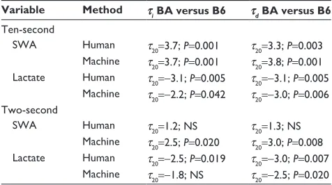
for independent measures yielded higher values for both parameters in the BA strain relative to the B6 strain, whether the scoring was automated or manual (τ₂₀.3.2; P,0.004, Table 5). The strain difference was inverted in the case of lactate-concentration dynamics across 10-second epochs; time constants for lactate were significantly reduced in BA mice relative to B6 mice (Figure 8E and F). Strain compari-son of lactate τi and τd via Student’s t-test for independent

measures yielded lower values for both parameters in the BA strain relative to the B6 strain, regardless of whether

10-second 2-second

Human Machine

<0.001

<0.001 0.009

0.010

NS

0.012 NS

NS

0.0 0.0

0.2 0.4 0.6 0.8 0.5 1.0 1.5 2.0 0 1 2 3 4 5 8

6

4

2

SWA

Time constant

τi

(hours)

SWA

Time constant

τd

(hours)

Lactate

Time constant

τi

(hours)

Lactate

Time constant

τd

(hours)

0

BA B6 BA B6

Strain Strain

F H

E G

B

A C

D

Figure 8 Strain differences in optimal time constants in general homeostatic modeling of state-dependent SWA and lactate dynamics.

Notes: Data represent optimized time constants for wake/REMS-dependent increases (τi) and SWS-dependent decreases (τd) in SWA (A–D) and lactate (E–H)

from human-scored data (black bars) and machine-scored data (gray bars). P-values are shown for main effect of scoring method on time constants.

Abbreviations: B6, C57BL/6J mice; BA, BALB/CJ mice; NS, not significant; REMS, rapid-eye-movement sleep; SWA, slow-wave activity; SWS, slow-wave sleep.

1,600

1,200

10-second

10-second 2-second

2-second

SWA

Residuals

(

µ

V)

SWA

Residuals

(

µ

V)

Lactat

e

Residuals

(

µ

A)

Lactat

e

Residuals

(

µ

A)

800

400

0

1,600

*

1,200

800

400

0

1.25

1.00

0.75

0.25

0.00

1.25

1.00 0.75

0.50 0.50

0.25

0.00

Strain

BA B6 NS NS

0.032 0.032

D C B A

Figure 9 Differences in residuals of model fit to data scored by human or machine.

Notes: Data represent the residuals associated with optimized time constants for modeling SWA (A and B) and lactate (C and D) from human-scored data (black bars) and machine-scored data (gray bars) in either 10-second or 2-second epochs.

P-values are shown for main effect of scoring method on time constants. Asterisk denotes significant difference for human versus machine scoring within the BA strain (Fisher’s protected least-significant difference).

Abbreviations: B6, C57BL/6J mice; BA, BALB/CJ mice; NS, not significant; R SWA, slow-wave activity.

Table 3 Strain difference in sleep timing: human versus machine

scoring

State Method BA versus

B6, minutes/ 24 hours

ANOVA (strain)

ANOVA (strain × time)

Wake human +38 NS F1,20=2.5; P,0.001

Machine +20 NS F_1,20=2.5; P,0.001

SWS human -14 NS F_1,20=2.6; P,0.001

Machine -1 NS F1,20=2.6; P,0.001

reMS human -24 F_1,20=27.0;

P,0.001

F_1,20=2.5; P,0.001

Machine -20 F_1,20=12.0;

P,0.002

F_1,20=2.5; P,0.001

Abbreviations: ANOVA, analysis of variance; B6, C57BL/6J mice; BA, BALB/CJ mice; NS, not significant; REMS, rapid-eye-movement sleep; SWS, slow-wave sleep.

(12)

the scoring was automated or manual (τ₂₀,–2.1; P,0.05, Table 5). Therefore, even in the presence of a bias toward longer time constants in the machine-scored dataset relative to the-human scored dataset, strain differences in the dynam-ics of both SWA and lactate were detected across 10-second epochs using both scoring methods.

80 Human

*

* * * * *

* * *

*

*** *** ***

***

* * * *

**

** **

Machine

Wake (%)

SWS (%)

REMS (%)

60

60 40

40 20

BA B6

20 0

0

0 4

E C

A B

D

F

8

20 0 4 8 12 16 20 20 0 4 8 12 16 20

Figure 10 Strain differences in sleep/wake state timing scored in 10-second epochs.

Notes: Strain differences in the time course of sleep/wake states were observed in human-scored data (A, C and E) or machine-scored data (B, D and F). Filled circles

represent data from the BA strain, and open circles represent data from the B6 strain. Asterisks indicate 60-minute epochs in which there is a statistically significant difference between strains (Fisher’s protected least-significant difference). Timing of the dark and light phases of the 12:12 cycle is indicated by the black and white bars at the top of each graph.

Table 4 Strain difference in 10-second EEG spectral profiles:

human versus machine

State Method ANOVA

(strain)

ANOVA

(strain × frequency)

Wake human NS F_19,380=4.3; P=0.001

Machine NS F_19,380=4.5; P=0.001

SWS human F_1,20=9.0; P=0.007 F_19,380=7.9; P=0.001

Machine F1,20=9.0; P=0.007 F19,380=7.8; P=0.001

reMS human NS F_19,380=12.8; P=0.001

Machine NS F19,380=12.8; P=0.001

Abbreviations: ANOVA, analysis of variance; NS, not significant; REMS, rapid-eye-movement sleep; SWS, slow-wave sleep.

5,000 4,500

Human

BA BA

B6 B6

Machine

4,000 3,500 3,000 2,500 2,000 1,500 1,000 500 0 5,000

3,000

NS NS

2,000 1,000 0

3,000 2,000 1,000 0 BA B6 BA B6 4,500

4,000 3,500 3,000 2,500 2,000 1,500 1,000 500 0 5,000 4,500 4,000 3,500 3,000 2,500 2,000 1,500 1,000 500 0

REMS

EEG power

(

µ

V

2/Hz)

SWS

EEG power

(

µ

V

2/Hz)

Wake

EEG power

(

µ

V

2/Hz)

C B

A D

E

F

Frequency (Hz)

4 8 12 16 20 4 8 12 16 20

Figure 11 Strain differences in EEG power spectra in 10-second epochs scored by human or machine.

Notes: The left column shows human-scored data and the right column shows machine-scored data. For wake (A and D), SWS (B and E), and REMS (C and F),

EEG power differed between strains at specific frequencies. The black dots at the base of each graph indicate frequency bands in which posthoc comparisons (Fisher’s protected least-significant difference) indicated a difference between the BA (black line) and B6 (gray line) strains. The insets in panels (B and (E) show 1–4 Hz SWA, which did not differ between strains.

Abbreviations: B6, C57BL/6J mice; BA, BALB/CJ mice; EEG, electroencephalography; NS, not significant; REMS, rapid-eye-movement sleep; SWS, slow-wave sleep.

The effect of strain on the temporal dynamics of both EEG SWA and lactate concentration across 2-second epochs was less statistically robust than for 10-second epochs (Table 5).

τd for lactate dynamics was the one parameter for which

both scoring methods yielded a significant effect of strain (Figure 8H). This parameter was significantly lower in BA

(13)

Table 5 Strain difference in homeostatic dynamics: human versus

machine

Variable Method τ_i BA versus B6 τ_d BA versus B6

Ten-second

SWa human τ20=3.7; P=0.001 τ20=3.3; P=0.003 Machine τ20=3.7; P=0.001 τ20=3.8; P=0.001 lactate human τ20=-3.1; P=0.005 τ20=-3.1; P=0.005

Machine τ20=-2.2; P=0.042 τ20=-3.0; P=0.006 Two-second

SWa human τ20=1.2; NS τ20=1.3; NS

Machine τ20=2.5; P=0.020 τ20=3.0; P=0.008 lactate human τ20=-2.5; P=0.019 τ20=-3.0; P=0.007

Machine τ20=-1.8; NS τ20=-2.5; P=0.020

Abbreviations: B6, C57BL/6J mice; BA, BALB/CJ mice; NS, not significant; SWA, slow-wave activity.

mice than in B6 mice, irrespective of state-scoring method (τ20,-2.4; P, 0.05, Table 5). For the other three parameters

assessed, Student’s t-test values for strain comparison were of equivalent direction (ie, positive for SWA and negative for lactate), if not statistically significant, for both state-scoring methods.

Discussion

This report introduces a novel method for automated scoring of sleep data. There were discrepancies between human-based and machine-human-based scoring, just as there are differences among human raters in state scoring. A more robust assess-ment of the automated scoring algorithm would compare it against two or more human scorers rather than just one. This would provide a measure of agreement not only between the algorithm and human scorers but also between one human scorer and another. This is a limitation of our approach.

Nonetheless, the utility of the machine-based scoring software introduced here is illustrated by its ability to detect strain differences in sleep-timing parameters, EEG spectral profiles, and sleep-dependent homeostatic variables. The machine-scored dataset detected strain differences in the percent of time spent in each sleep state with hourly resolu-tion; the timing of these strain differences with respect to the light/dark cycle replicated their timing in the human-scored dataset (Figure 10). The strain differences in EEG spectral power that were detected in the human-scored dataset were replicated precisely, at the level of 1 Hz intervals, in the machine-scored data. Strain differences in time constants associated with sleep-dependent dynamics of SWA and lactate were of equivalent magnitude and direction in the human-scored and machine-scored datasets. Although all of these parameters (sleep-state timing, EEG power spec-tral profiles, time constants in homeostatic models) varied

significantly between the human-scored and machine-scored datasets, scoring method and strain did not exhibit signifi-cant interaction in affecting these variables. Thus, the bias in machine-based state scoring was not strain-specific, and strain differences were not lost in the automation process. To the extent that the purpose of state scoring is to detect effects of independent variables on sleep parameters, the automated scoring algorithm introduced here fulfills its purpose in detecting strain differences.

Machine learning alone was not sufficient to accurately score REMS. Some epochs scored as wake by human experts were scored as REMS when automated scoring was based solely on PCA of epochs in isolation. Human raters use contextual cues, specifically the fact that REMS is consis-tently preceded by a protracted period of SWS in wild-type mice, to discriminate REMS epochs from wake epochs characterized by low EMG and EEG amplitudes occurring against a background of continuous wake. Therefore, we applied contextual information in the algorithmic scoring of REMS: episodes scored as REMS that were preceded by at least 30 seconds of wake were rescored as wake. While not as parsimonious as state scoring based solely on EEG and EMG features of each epoch, this logic replicates the use of contextual information by human experts and in any case increases the level of agreement with human scoring. In experimental circumstances when direct transitions from wake to REMS are expected to occur (such as studies on narcoleptic hypocretin-deficient mice30,31_{), the algorithm}

might be altered to ﬂag the occurrence of such events within the MATLAB interface, allowing for visual inspection and verification of such transitions. However, in the current study of wild-type mice, this consideration is not relevant. Also, while the choice of 30 seconds is reasonable, we acknowl-edge that it is somewhat arbitrary. In principle, one could determine the optimal amount of preceding wake to use in this rescoring rule by testing several different values and determining the best fit to human-scored data.

We chose to combine the PCA approach with a naïve Bayes classifier because it offers several benefits over other methods. In fact, this was first suggested in a previous study as a possible improvement to current approaches.2_{First of}

all, the method is easy to implement in MATLAB using the built-in functions pca.m and classify.m. Second, this approach combines the appealing visualization properties of PCA with the power and efficiency of machine learning. A researcher can visually inspect the effectiveness of the machine scor-ing by lookscor-ing at the EEG and EMG traces aligned with the machine score and by looking at the PCA plots of the

(14)

human-scored data and the machine-scored data. Because the method requires scoring a small subset of each data file, this hybrid method is relatively simple, requires only a small subset of each data file to be scored to train the algorithm, and does not overfit the data. We have shown good agree-ment between human-scored data and machine-scored data when only 10% of the dataset is scored by hand and used as training for the algorithm. Since the algorithm runs in less than 30 seconds for a 43-hour dataset, the time required to score an entire dataset using this automated approach is about one tenth of the time it would take to score the entire recording by hand.

implications of 2-second versus

10-second epoch length and scoring

method on time constants for EEG

and lactate dynamics

Using a homeostatic model to quantify EEG SWA dynamics with 10-second epochs scored by a human, we previously found optimal τi values that were significantly smaller than

those computed by other groups.16_{To our knowledge, the}

experimental setup was identical between our recordings and those of Franken et al,16_{except for the fact that we used}

an epoch length of 10 seconds and Franken et al used an epoch length of 4 seconds. Because epoch length was the only experimental difference we could find, we speculated that the epoch length may impact the optimal values of the time constants chosen to fit the model to the data. When fit-ting the model to SWA data (as in Figure 7E–H) following Franken et al,16_{each data point represents the average delta}

power in a 5-minute segment that contained at least 90% SWS. We suspected that the epoch length may affect these data points in the following ways: if a 10-second epoch was part SWS but part wake, the scorer may score it as SWS. Using a finer resolution, a scorer may determine that not all of those 10 seconds should be scored as SWS, which may mean that some 5-minute segments that used to contain at least 90% SWS were actually less than 90% and therefore would not create a data point for that 5-minute segment. On the other hand, if some 10-second epochs that were scored as wake actually had some SWS, this may create new data points because there may be 5-minute segments that now have 90% SWS. Because changing epoch length could add or remove data points, we reasoned that it may alter the time constants of the optimal fit of the model.

The autoscoring algorithm allowed us to quickly rescore 10-second epoch data into 2-second epochs, so we could run homeostatic models on the 2-second data to test

this hypothesis. We found that running the model using a shorter epoch length (2 seconds) did indeed increase the optimal τi values for both strains, making them closer to

those found in Franken et al.16_{However, the optimal value}

of τd did not change for either strain as a function of epoch

duration. Application of the automated scoring and model-ing techniques to both lactate and SWA in a broader array of strains (like those used by Franken et al16_{) may reveal}

whether sleep-dependent dynamics of lactate correlate with sleep timing or electroencephalographic parameters.

Conclusion

We have demonstrated that our machine-scoring algorithm is as effective as human scoring in several different aspects. Various measures of agreement between human scoring and machine scoring were high, and the machine scoring algorithm was just as effective as human scoring in deter-mining subtle differences between genetic strains in both the frequency domain and the time domain. As scoring an entire multiday recording requires less than a minute of computing time (even for 48 hours of 2-second epoch data), automated scoring is a very efficient alternative to visual inspection in rodent sleep studies and may be similarly effective with sleep data from other species, including humans.

Acknowledgments

We thank Jonathan P Brennecke for technical assistance. This work was supported by National Institute of Neurological Disorders and Stroke award R01 NS078498 and National Institute of Drug Abuse award R21 DA037708. The authors declare that they have no additional financial support for this work and no off-label or investigational use. All work was performed at Washington State University, Spokane.

References

1. Stephenson R, Caron AM, Cassel DB, Kostela JC. Automated analysis of
sleep-wake state in rats. J Neurosci Methods. 2009;184(2):263–274.
2. Gilmour TP, Fang J, Guan Z, Subramanian T. Manual rat sleep
clas-sification in principal component space. Neurosci Lett. 2010;469(1):
97–101.
3. Rytkönen KM, Zitting J, Porkka-Heiskanen T. Automated sleep scoring
in rats and mice using the naive Bayes classifier. J Neurosci Methods.
2011;202(1):60–64.
4. Brankack J, Kukushka VI, Vyssotski AL, Draguhn A. EEG gamma frequency and sleep-wake scoring in mice: comparing two types of
supervised classifiers. Brain Res. 2010;1322:59–71.
5. Gross BA, Walsh CM, Turakhia AA, Booth V, Mashour GA, Poe GR. Open-source logic-based automated sleep scoring software using
elec-trophysiological recordings in rats. J Neurosci Methods. 2009;184(1):