Channel Modeling Network Analysis In Sea Water
Medium For High Speed Using EM Waves
Gursewak Singh, Mahendra Kumar
Abstract: In this paper, channel modeling for velocity control of electromagnetic (EM) waves in water medium through some characteristics such as characteristics impedance of EM waves, refractive index, and electrical conductivity of sea water was analyzed and examined with help of some mathematical tools under simulation process to meet practical specifications. The main problem in underwater wireless communications is the slow speed of available acoustic communication. On the other side, acoustic communication has low data rate capability because of low frequency employment for acoustic signal. One of alternative solution to avoid this problem such as slow speed is an employment of Electromagnetic waves in water medium. The EM waves in water provide us platform of high speed and high data rate at high frequency. The main purpose of this paper was to examine the underwater EM communication network, its feasibility and applicability in underwater wireless communication (UWC). Based on observations, a channel model of EM high speed in underwater medium was designed and implemented using EM waves at high frequency. This development of speed channel model for water medium provides a high speed EM communication technology in underwater channel.
Keywords: Electromagnetic wave propagation; Refractive index; High-Frequency Effects; Impedance; Velocity measurement.
————————————————————
1.
INTRODUCTION
In today era, an abundant attention is being paid on evolution of underwater wireless communication network technology. Underwater wireless communication Network technology is being achieved through many communication methodologies such as acoustic communication, optical communication, electromagnetic (EM) communication [1-4]. The acoustic wireless communication technology has low data rate capacity and high propagation delay such as speed (1500m/s) as compared to electromagnetic communication. The propagation latency in wireless communication due to slow speed which does not helps the underwater wireless communication system to work in fast and optimal manner. Acoustic waves have very low data rate capability and impractical for real-time target tracking system. Moreover, acoustic data communication has high bad impact on marine life [2]. In these types of wireless networks, a web of many sensor nodes is spread and designed to transfer the information from one place to another side for achieving many real time target applications [5-7]. Alternative solution to these problems is employment of EM technology [8-9] which has high data rate capability, high speed of communication over short range and no bad impact on marine life which is part of our nature. Using EM waves, marine life can be protected very high level as compared to acoustic and optical waves [8-9]. The electromagnetic (EM) waves in the radio frequency (RF) range can also be employed for wireless underwater communication systems. The velocity of EM waves in underwater medium is 4 times quicker than acoustic waves, so there is great reduction in the channel latency. Additionally, EM wave’s sensitivity to reflection and refraction influence is less than acoustic waves in shallow water. Few underwater wireless communication systems based on EM waves have been proposed before [10-11]. The speed of EM wave mostly depends upon ( ) permittivity of medium, ( )
conductivity of water medium, ( ) permeability of medium [12].
Usual RF transmission performs badly in seawater owing to the losses generated by the high conductivity of seawater (normally, 4 S/m) [13]. The latency in channel produced by the low velocity of propagation in water is a limitation of acoustic communications [14].A substitute clarification to these problems is use of EM technology [9] Objective of this research paper is to examine its feasibility and velocity of electromagnetic waves in water medium. From here, the research paper is organized as follows. In Sect. 2, related work for mathematically design of channel model for velocity of propagation speed was introduced. In Sect. 3, Graphical performance results were observed. Finally, the work of this paper is concluded in Sect. 4.
2.
DESIGN AND DEVELOPMENT OF SPEED
CHANNEL MODEL
In this section, the velocity of propagation model was developed after using some significant parameter such as absolute value of characteristics impedance of EM waves. The speed of EM waves in sea water medium will be examined which depends upon frequency and electrical conductivity of medium.
2.1 Design and Development of Speed Channel Model through characteristics impedance of EM waves As it is known that the waves can be expressed as cyclic energy variations in form of information, eg. EM waves, Microwaves, light rays, TV signals etc . The main benefits of using electromagnetic waves instead of acoustic waves reducing the latency due to faster propagation and achieving a high data rate due to use of high frequency of the wave [15].EM waves consist of electric and magnetic field which are perpendicular to each another during its journey in any medium. In this work, speed channel model in water medium using EM waves will be designed and developed through mathematical tools such as exponential theory, vector theory and EM wave’s characteristics etc. In Fig. (1), a sinusoidal waveform of electrical field of EM waves is considered whose mathematical expression can be written below in form of eq. (1). [21, 26]. The waveform travels in y-axis direction.
p
p
_____________________
Research scholar, Guru Kashi University, Talwandi Sabo, Punjab, India,
X-axis
( , )
y t
o
t Y-axis
2
Fig 1.Sinusoidal EM wave
o
sin(
p( y,t )
)
(1) Where
o
is amplitude of sinusoidal waves and(
p)
isphase angle,
is wavelength,( , )
y t
is electric field of EM signal, t is time.Phase constant (Pc) can be defined as ratio of total angle of one cycle
2
360
0
and wavelength (
) which can be expressed in eq. (2) [16-17].2
Pc
(2)Velocity of wave
v
wave
can be expressed as ratio of change in displacement waves in y-axis direction w.r.t change in time given below as shown in Fig. (1) and eq. (3) [16-17]
wave
dy
v
dt
(3)Angular frequency (
) can be expressed as given below in form of eq. (4) by [16-17]
Pc v
wave
(4)
Using above eq. (2), eq. (3) and eq. (4), following formula can be derived such as in form of eq. (5) given below [16-17].
2
.
dy
.
dt
(5)Integrating [18] equation (5) to both sides, following expression can be obtained in form of eq. (6) and eq. (7).
2
.
dy
.
dt
(6)2
.
y
.
t
p
(7) Where
(
p)
is phase angle,
is wavelength ,When there is change in phase on sine waves, then phase angle
2
-
p
y
t
from equation (7) can beplaced in eq. (1) to obtain eq. (8) [16-17]
02
sin
( y,t
)
y
-
t
(8)Above eq. (8) can be re-written as below in form of eq. (9) in cosine waveform after changing phase
p by angle (900) [16-17]
0
( y,t )
cos
t
2
y
(9)
As per Euler identity by [16-17] given below in form of eq. (10).
j( p)
p p
e
cos
j sin
(10)
Putting phase angle
2
p
t
y
in eq. (10), Euler identity can be written in real part (Re) and imaginary part (Im) as below in form of eq. (11).
2j t y
2
cos
t
y
e
2
j sin
t
y
(11)
Above eq. (9) of electric field
( , )
y t
can be re-written as below in form of eq.(12) using Euler identity eq. (11). 2
j t y
0
( y,t )
Re e
Partial differentiation [18] of above eq. (12) can be performed w.r.t time (t) to obtain eq. (13), eq. (14)
2
j t y
0
' '
( y
)
Re e
t
,t
t
(13)
Rewrite above eq. (13) in form of eq. (14) after putting eq. (12) in eq. (13).
'
( y,t
j
t
)
( y,t )
(14)Equating eq. (14) to both side to express equation (15) below.
'
j
t
(15)Partial differentiation [18] of above eq. (12) can be performed w.r.t time (y) to obtain eq. (16) and eq. (17).
2
j t y
o
( y,t )
Re e
y
y
(16)
Rewrite above eq. (16) in form of eq. (17) after putting eq. (12) in eq. (16).
o( y,t )
( y,t ) 2
j y
p l ®
®
æ ö
¶Î ç ÷
Î = -ççè ÷÷ø* 
V
V (17)
In similar manner, Magnetic field ( , )
H y t varies in y-axis
direction as electrical field varies shown in eq. (12) and Fig. (1).
'
2
j t y
0
H( y,t )
H
Re e
(18)
Partial differentiation [18] of above eq. (18) can be performed w.r.t time (y) to obtain eq. (19) and eq. (20).
2
j t y
0
H( y,t )
Re e
y
y
H
(19)
Rewrite above eq. (19) in form of eq. (12) after putting eq. (18) in eq. (19).
( y,t )
H( y,
H 2
j t )
y
p l
®
æ ö
¶ ç ÷
= -ççè ÷÷ø* 
V
V
(20)
To calculate the velocity of EM waves in water medium, Maxwell equations from [21] will be used and written as below in form of eq. (21) and eq. (22).
( , )
-
( , )
pH y t
t
y t
(21)
( , )
( , )
( , )
p
y t
y t
H
y t
t
(22)
Where;
pis permittivity of water medium,( , )
y t
is electricfiled intensity ,
( , )
H y t
is magnetic field intensity,
pis permeability of water medium,
is conductivity of watermedium, j
t
from equation (15) [21] .
Re-write above eq. (21) in form of eq. (23) after putting eq. (15) in eq. (21) .
-
( ,
( , )
)
y
t
j
pH
y t
(23)Rewrite above eq. (22) in form of eq. (24) after putting eq. (15) in eq. (22).
( , )
( , )
H
y
t
j
p
y
t
(24)
magnetic field in z-axis direction as represented by eq. (26) [21]. x-axis f x
l
( , )
y t
f
y
l y-axis
f
z
l z-axis
H y t
( , )
®
Fig 2 vector representations in x-axis, y-axis, z-axis direction
x x
(
l
,t )
( y,t )
l
® ®
Î
=
Î
(25)
z z
H(l ,t ) H( y,t )l
® ®
= (26)
The curl of a vector field
( , )
y t
revealed as ( y,t ) ® »Ñ δ
can be written as below in form of vector representation as in eq. (27) matrix form with help of drawn Fig. (2), which is circulation or rotation of vector field in all directions [21].
" '
x y z
x
y z
x y z
( y,t )
( y,t ) ( y , ( y,t ) 0 0
-z y
t )
l l l
l l l » ® ® ® ® ¶ ¶ ¶ = ¶ ¶ ¶ æ ö çÑ´ ÷ = ç ÷ ç ÷ è ø Î Î ¶ Î Î ¶ ¶ 
V V V
V V V
V V
V V
(27)
As shown in Fig. (2), vector electric field
( , )
y t
component in x- axis direction. So, change in electric field
( , )
y t
component is shown in x-axis direction as shown in Eq. (28) in matrix form [21].
x y z
x z
" '
-x y z y
(
( y ,t ) (
y,t ) 0
y,t )
0
l l l
l l » ® ® ® æ ö ¶ ¶ ¶ ¶ çÑ´ Î ÷ = = Î ç ÷ ç ÷ è ø ¶ ¶ ¶ ¶ Î
V V V V
V V V V
(28)
Compare above eq. (23) and eq. (28) to obtain eq. (29)
( y,t ) - j p
y
H( y,t )
m w ® ® æ ö ¶ ç ÷ = çç ´ ´ ÷÷ è ø ¶ Î V V (29) Compare above eq. (17) and eq. (29) to obtain eq. (30).
p 2
j p ( y,t ) - jm w H(y,t)
l ® ® æ ö æ ö ç- ÷* ç ´ ´ ÷ ç ÷ çç ÷÷ ç è ø
è ø÷ Î = (30)
In similar manner, as shown in Fig. (2), vector magnetic field
( , )
H y t
component in z-axis direction. The change in magnetic field( , )
H y t
component is shown in z-axis direction as curl representation H( y,t )» ®
Ñ´ shown in Eq. (31) in matrix form [21]
x y z
z x
H( y,
x y z
t ) H(
y
0 0
y,t )
H( y,t )
l l l
l l » ® ® ® æ ö ¶ ¶ ¶ ¶ çÑ´ ÷ = = ç ÷ ç ÷ è ø ¶ ¶ ¶ 
V V V V
V V V V
(31) Compare above eq. (24) and eq. (31) to obtain eq. (32).
(
)
{
p}
H( y,t )
( y,t - j y ) d we ® ® É ¶ Î = + ¶ V V (32) Compare above eq. (20) and eq. (32) to obtain eq. (33).
(
)
{
p}
H( y,t ) ( y,t
j2p - d jwe )
l ® ® É æ æ öö ç- ç ÷÷* = + ç ç ÷÷ ç ç ÷÷ ç è ø÷ è ø Î (33) Divide eq. (30) and eq. (33) to obtain eq. (34)
(
)
{
}
p
p
( y,t ) H( y,
2
j - j t )
( y,t ) 2
H( y, ) j
j t
-p
m w
l
p d we
l É ® ® ® ® æ æ öö ç- ç ÷÷* * * ç çç ÷÷÷ ç è ø÷ è ø = æ ö æ ö ç ÷ Î ç ÷ æ ö ç- ç ÷÷* + ç ç ÷÷ ç ÷ è ø Î ç ÷ ç è ø÷ è ø (34)
After cross-multiplying eq. (34), following equation will be obtained as given below in form of eq. (35) and eq. (36).
(
)
(
)
p p 2 2( y,t )
( y,t )
j
j
H
m
w
d
we
® ® É*
+
Î
=
(35)(
)
(
)
p p ( y,t )( y,t ) j j H m w d we ® É ® * + Î = (36)
The Characteristics impedance (
) of EM wave can be defined as ratio of transverse components of the electric field and magnetic fields. The Characteristics Impedance (
) of EM wave is given in form of eq. (37) with help of eq. (36) [21].
( , )
( , )
p
1 2 1
2
1
p p
p
p p
j
j
j
j
j
(38) Where;
2
f
is angular frequency and
f Is frequency of signal.
p Is permittivity of medium,
is conductivity of water medium,
pis permeability of medium.Good conductor medium at conditions given in eq. (39) and eq. (40) [21] as;
1
p
(39)
0
, ,
upto p p o (40)
As per above characteristics discussed, channel model designing will be performed of EM waves in water medium. Considering high conductive medium and after applying condition from eq. (39) on eq. (38), following eq. (41) for characteristic impedance (
) will be achieved after separating its real ( ) and imaginary (
)components.
1 2
p
j
j
(41)
After squaring both side of eq. (41), following eq. (42) will be achieved.
2 2
2
p
j
j
(42)Separate the real and imaginary part of eq. (42), following eq. (43) and eq. (44) will be achieved given below.
2 20
(43)
2
p
(44) The real part (
) and imaginary part (
) ofcharacteristic impedance (
) will be obtained as below in form of eq. (45).
2
p
(45) Add the real part (
) and imaginary part (
) ofcharacteristic impedance (
) to calculate absolute value of Characteristics impedance (
) in equation (46)
which is to be considered in this research paper for finding real value of velocity of propagation of EM waves in water medium.
2
p
(46)
As, it is known from [20-23], the absolute value of Characteristics impedance (
) can also be written
below in form of equation (16).
0
r r
(47) Where(
) is absolute value of characteristics impedance, ( 0
) is absolute value of characteristics impedance in freespace, (
) is Refractive index, (
r) is relative permeability.As water is non magnetic medium, its relative permeability
r
r
is 1,and characteristics impedance0
376.8
ohm
is same as in free space [20-23], above eq. (47) can be re-written below in form of eq. (48) for absolute value of Characteristics impedance (
).
376.8
(48)
Refractive index (
) [21, 23-24] in eq. (49) can
be defined as ratio of velocity of light in free space (Such as c= 3x10⁸m/s) [21, 23-24] and (
V
) velocity in medium.
c
V
(49)
8
2
3 10
376.8
p
V
(50)
As from eq. (40), water is non magnetic medium; its
7
0
4
10
p
permeability is same as freespace.
2
f[19, 21, 26]Re-write above equation (50) in form of eq. (51) after putting
p
04
10
7,
2
f[19, 21, 26].7 14
10
10
3 10
4
376.8
fV
(51)As numerator part in eq. (51) calculated
3.14
3 10 4
376.8
value to put in eq. (51) to obtain equation (52).The value of velocity of propagation of EM waves in water medium from equation (51) which depends upon conductivity (
) of water medium and frequency (f
) of EM signal.7
10
f
V
(52) 2.2 Electrical conductivity (
) of sea waterThe performance of Electromagnetic waves in underwater environment depends on the accuracy of electrical conductivity of sea surface. Moreover, the Electromagnetic absorption due to water depends upon the electrical conductivity
of sea water measured in laboratory experiments given by equation (53) [27-28].
1 1 3 2
0 1 1 2
1 2 2 2
2 2
2 2 2 2
374 10
54 10
16 10
10058 10
1819 10
69 10
331 10
12 10
15
8461 10
69
1
4980 10
24 10
20 10
S
S
S
S S
S
S
T
S S
S
S
T
(53)
3 5 2
0 7 3 10 4
2.90 86 10 47 10
30 10 43 10
T T
T T
(54) Where
(T) is temperature is in degrees centigrade, (S) is salinity in PPT (parts per thousand),
is electrical conductivity in Siemens per meter.
0 is the electrical conductivity at S = 35 PPT and is given in dependence of temperature.The electrical conductivity of sea water calculated from mathematical experimental results depends upon salinity and temperature of underwater environments as derived in equation (53) by [27-28].
3.
RESULTS AND DISCUSSION
In this section, an examination on velocity of propagation in sea water medium was done by finding different results
through plotting figures and 3 D graphs which will analyze the velocity of propagation with variations of salinity (S) and temperature (T).
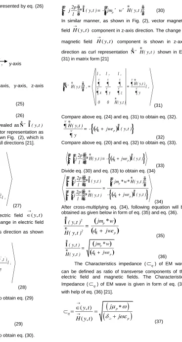
Fig 3 Velocity of propagation Vs conductivity and frequency
As shown in Fig. (3) and Table (1), at salinity 25PPT and frequency 300MHz, 400MHz, 500MHz, 600MHz, the
electrical conductivity is
3.8963(S/m),4.2852(S/m),4.6825(S/m),5.0870(S/m).At salinity 25 PPT, The characteristics impedance is 34.8517(ohm), 38.3738(ohm), 41.0426 (ohm) 43.1354(ohm). The Velocity of propagation is 2.7748x10⁷(m/s),3.0552x107(m/s),3.2677x107(m/s), 3.4343 x10⁷(m/s). As shown in Fig. (3) and Table (1), at salinity 35PPT, and frequency 300MHz, 400MHz, 500MHz, 600MHz electrical conductivity is 5.2741(S/m), 5.7986(S/m), 6.3342(S/m), and 6.8791(S/m).The Characteristics impedance is 29.9554(ohm), 32.9881(ohm), 35.2880(ohm), and 37.0935(ohm). The Velocity of propagation is 2.3850x10⁷(m/s), 2.6264x10⁷(m/s), 2.8096 x10⁷(m/ s) and 2.9533 x10⁷(m/s). As shown in Fig. (3), at salinity 40PPT, and frequency 300MHz, 400MHz, 500MHz, 600MHz, electrical conductivity is 5.94199(S/m), 6.5324(S/m), 7.1353(S/m) and 7.7487(S/m). The Characteristics impedance is 28.2219(ohm), 31.0801(ohm), 33.2481(ohm) and 34.9504(ohm). The Velocity of propagation is 2.2470x10⁷(m/s), 2.4745 x10⁷(m/s), 2.6471x10⁷(m/s), and 2.7827 x10⁷(m/s).
3 4
5 6
x 108 2
4
6
8 2
2.5 3 3.5 4
x 107
Frequency(Hz) velocity(m/s) in sea water
cond(S/m)
v
e
lo
c
it
y
(m
/s
Fig 4 Velocity of propagation Vs frequency at fixed temperature
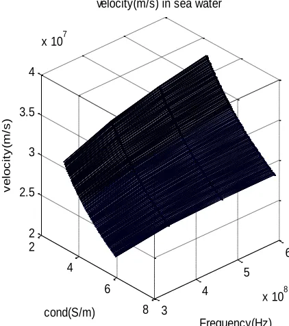
It can be observed from Fig. (3) and Table (1) that at fixed salinity and by increasing frequencies, the characteristics impedance increases which cause the increase in velocity of propagation. If salinity increases, the electrical conductivity increases, the characteristics impedance decreases which cause the decrease in velocity of propagation. The velocity of propagation increases by increasing frequency. On the other side, the velocity of propagation decreases by increasing electrical conductivity. As shown in Fig. (4), at salinity 30 PPT and temperature 25
0
C, at different frequency 300MHz, 400MHz, 500MHz, 600MHz, the electrical conductivity is 4.5927(S/m). Characteristics impedance is 32.1008(ohm), 37.0668(ohm), 41.4420 (ohm), 45.3974(ohm). The Velocity of propagation is 2.5558x10⁷ (m/s), 2.9512x10⁷(m/s), 3.2995x10⁷(m/s), 3.614x10⁷(m/s).
As shown in Fig. (4), at salinity 20 PPT and temperature 25
0
C, at different frequency 300MHz, 400MHz, 500MHz, 600MHz, the electrical conductivity is 3.1831(S/m).The Characteristics impedance is 38.5589(ohm), 44.5240(ohm), 49.7793(ohm),54.5305(ohm).Velocity of propagation is 3.0700x10⁷(m/s), 3.5449x10⁷(m/s), 3.9633x10⁷(m/s), 4.3416x10⁷(m/s). It can be observed from Fig. (4) that at fixed salinity and fixed temperature, by increasing frequencies, the characteristics impedance increases which cause the increase in velocity of propagation. If salinity increases, the electrical conductivity increases, the characteristics impedance decreases which cause the decrease in velocity of propagation. As shown In Fig. (4), the salinity increase from 20PPT to 30PPT, the velocity of propagation decreases at each step of same frequency.
Fig 5 Velocity of propagation Vs frequency at fixed salinity
Table 1 Velocity of propagation at different temperature, salinity and frequencies
At Salinity =25 PPT Sea water Sea water Sea water Sea water
Temperature (T) (0C) 25(0C) 35(0C) 35(0C) 45(0C)
Frequency
f (MHz) 300 400 500 600Velocity of propagation (ms-1) 2.7748 X10⁷ 3.0552 X10⁷ 3.2677 X10⁷ 3.4343 X10⁷
Electrical conductivity
(S m-1) 3.8963 4.2852 4.6825 5.0870Characteristics impedance
(ohm) 34.8517 38.3738 41.0426 43.1354
3 4 5 6
x 108 0
0.5 1 1.5 2 2.5 3 3.5 4 4.5x 10
7
v
e
lo
c
it
y
(m
/s
)
Frequency(Hz) velocity(m/s) in sea water
S=30PPT T=25 *C
S=20PPT T=25 *C
3 4 5 6
x 108 0
0.5 1 1.5 2 2.5 3 3.5 4 4.5x 10
7
v
e
lo
c
it
y
(m
/s
)
Frequency(Hz) velocity(m/s) in sea water
S=20PPT T=30 *C
At Salinity =35 PPT Sea water Sea water Sea water Sea water
Velocity of propagation (ms-1) 2.3850X10⁷ 2.6264X10⁷ 2.8096 X10⁷ 2.9533 X10⁷
Electrical conductivity
(S m-1) 5.2741 5.7986 6.3342 6.8791Characteristics impedance
(ohm) 29.9554 32.9881 35.2880 37.0935
At Salinity =40 PPT Sea water Sea water Sea water Sea water
Velocity of propagation (ms-1) 2.2470 X10⁷ 2.4745 X10⁷ 2.6471 X10⁷ 2.7827 X10⁷
Electrical conductivity
(S m-1) 5.9419 6.5324 7.1353 7.7487Characteristics impedance
(ohm) 28.2219 31.0801 33.2481 34.9504
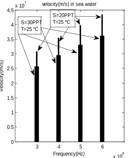
At salinity 20PPT and temperature 300C, as shown in Fig. (5), at different frequency 300MHz, 400MHz, 500MHz, 600MHz, the electrical conductivity is 3.5021(S/m).The Characteristics impedance is 36.7608(ohm), 42.4477(ohm) , 47.4579(ohm), 51.9876(ohm). The Velocity of propagation is 2.9268x10⁷(m/s), 3.3796x10⁷ (m/s), 3.7785x10⁷(m/s), 4.1391x10⁷(m/s). It can be observed from Fig. (5) that at fixed salinity and fixed temperature, by increasing frequencies, the characteristics impedance increases which cause the increase in velocity of propagation. If salinity fixed, the temperature increases which cause the electrical conductivity increases, the characteristics impedance decreases which further cause the decrease in velocity of propagation. In Fig. (5), the salinity fixed 20PPT but temperature increases from 25oC to 30oC, the velocity of propagation decreases at each step of same frequency. At salinity 20PPT, 30PPT, 35PPT, 40PPT and temperature 25 0C and frequency 400MHz, as shown in Fig. (6), at frequency 400MHz, the electrical conductivity is 3.8939(S/m), 4.5918(S/m) 5.2744(S/m), 5.9430(S/m). The Characteristics impedance is 40.2555(ohm), 37.0703(ohm), 34.5887(ohm), 32.5849(ohm). The Velocity of propagation is 3.2051x10⁷ (m/s), 2.9515 x10⁷(m/s), 2.7539x10⁷(m/s), and 2.5943x10⁷(m/s). At salinity 20PPT, 30PPT, 35PPT, 40PPT and temperature 25 0C and frequency 600MHz, as shown in Fig. (6), The electrical conductivity is 3.8939 (S/m), 4.5918(S/m), 5.2744(S/m), 5.9430(S/m). Characteristics impedance is 49.3027 (ohm), 45.4017(ohm), 42.3623(ohm), and 39.9082(ohm). The Velocity of propagation is 3.9254x10⁷(m/s),3.6148x107(m/s),3.3728x107(m/s),3.1774x 107(m/s).
Fig 6 Velocity of propagation Vs salinity at fixed temperature and frequency
As, It can be observed from Fig. (6), at fixed temperature and increment in salinity, the velocity of propagation decreases at fixed frequency. On the other side, at fixed temperature and increment in salinity, the velocity of propagation decreases at fixed frequency. However, by increasing frequency from 400 MHz to 600MHz, the velocity of propagation increases.
4.
CONCLUSION
In this work, feasibility and applicability of propagation of electromagnetic (EM) wave in water medium was examined through designing and development of speed channel model for electromagnetic wave. The employment of EM waves at high frequency which causes the faster propagation of EM waves in water medium with low
20 25 30 35 40
2.5 3 3.5 4 4.5x 10
7
v
e
lo
c
it
y
(m
/s
)
salinity(S)(PPT) velocity(m/s) in sea water
400MHz 600MHz S=20:5:40 PPT
propagation delay and low latency. Mainly, channel propagation speed model was designed through mathematical tools which provide us real feasibility for propagation of EM waves in water medium. Based on observations, high speed of underwater communication in sea water medium was designed and developed using EM waves at high frequency. The velocity of propagation decreases with increase of electrical conductivity by increasing temperature in sea water medium at fixed frequency level. The proposal of high speed model provides high speed communication technology at high frequency. Velocity of propagation decreases with increase of electrical conductivity by increasing temperature in sea water medium at fixed frequency level. On the others hand, It can be seen, if frequency level is increased from 300 MHz to 600MHz at fixed salinity, the velocity of propagation increases. However, by increasing temperature, the electrical conductivity increases which cause the decreases in velocity of propagation sea water medium. Finally, it can be observed that velocity of propagation increases by increasing the frequency. The employment of high frequency which causes the faster propagation of EM waves in water medium with low propagation delay and low latency.
ACKNOWLEDGEMENTS
I would like to thank to Dr. Mahendra Kumar, Dy.Dean Research, Department of ECE, GKU, constant support and encouragement to carry out this innovative work. His support, guidance and confidence boosted my abilities to perform this project successfully.
REFERENCES
[1] X. Che, I. Wells, P. Kear, G. Dickers, X. Gong, and M. Rhodes, ―A static multi-hop underwater wireless sensor network using RF electromagnetic communications,‖ in Proc. 2009 IEEE Int. Conf. on Distributed Computing Systems Workshops, pp. 460–463.
I. F. Akyildiz, D. Pompili, and T. Melodia, ―Underwater acoustic sensor networks: Research challenges,‖ Ad Hoc Networks, vol. 3, no. 3, pp. 257– 279, 2005.
[2] D. Anguita, D. Brizzolara, and G. Parodi, ―Building an underwater wireless sensor network based on optical communication: research challenges and current results,‖ in Proc. 2009 IEEE Int. Conf. on Sensor Technologies and Applications, pp. 476– 479.
[3] SArnon,―Underwater optical wireless communication network‖ Optical Engineering 49(1), 015001,January 2010.
[4]
K, Munasinghe, M Aseeri, S.Almorqi, M. F Hossain, M B Wali, and A Jamalipour (2017), EM-Based High Speed Wireless Sensor Networks for Underwater Surveillance and Target Tracking, Journal of Sensors, Vol 2017,pp.1-14,https://doi.org/10.1155/2017/6731204
[5] L. Liu, S. Zhou, and J.-H. Cui,(2008), Prospects and problems of wireless communication for underwater sensor networks, Wireless Communications and Mobile Computing, vol. 8, no.
[6] ]J.-H. Cui, J. Kong, M. Gerla, and S. Zhou,(2006), The challenges of building scalable mobile underwater wireless sensor networks for aquatic applications, IEEE Network, vol. 20, no. 3, pp. 12– 18, 2006.
[7] X. Che, I. Wells, G. Dickers, P. Kear, and X. Gong, ―Re-evaluation of RF electromagnetic communication in underwater sensor networks,‖ IEEE Communications Magazine, vol. 48, no. 12, pp. 143–151, 2010.
[8] ]Kumudu. M., Mohammed. A., and Sultan. A., (2017), ― EM-Based High Speed Wireless Sensor Networks for Underwater Surveillance and Target Tracking,‖ Hindawi Journal of Sensors , pp.1-14, https://doi.org/10.1155/2017/6731204.
[9] J. H. Goh, A. Shaw, A. I. Al-Shanmma’a, ―Underwater Wireless Communication System,‖ Journal of Physics, Conference Series 178, 2009. [10]]A. I. Al-Shamma’a, A. Shaw and S. Saman,
―Propagation of Electromagnetic Waves at MHz Frequencies through Seawater,‖ IEEE Transactions on Antennas and Propa- tion, Vol. 52, No. 11, November 2004, pp. 2843-2849.
[11]Chakraborty, U.; Tewary, T.; Chatterjee, R.P. Exploiting the loss-frequency relationship using rf [12]communication in underwater communication
networks. In Proceedings of 4th International Conference on Computers and Devices for Communication, CODEC 2009, Kolkata, India, [13]14–16 December, 2009..
[14]S. Bogie, ―Conduction and Magnetic Signaling in the Sea,‖ Radio Electronic Engineering, Vol. 42,
No. 10, 1972, pp.
447-452.doi:10.1049/ree.1972.0076.
[15]L. Liu, S. Zhou and J. Cui, ―Prospects and Problems of Wireless Communication for Underwater Sensor Net-works,‖ Wiley WCMC Special Issue on Underwater Sen-sor Networks (Invited), 2008.
[16]Lloret, J., Sendra, S., Ardid, M., and Rodrigues, J.,
(2012), Underwater Wireless Sensor
Communications in the 2.4 GHz ISM Frequency Band, 3(12), pp.4237–4264.
[17]Mihir,S.,(2014), Introduction to the Mechanics of Waves, pp.1-70
[18]Georgi, H .,(1993), The Physics of Waves, Prentice hall,USA,pp.1-465.
[19]Michael, S.,(1965 ), Calculus on Manifolds, A modern approach to classical theorems of advanced calculus, Addison-Wesley Publishing Company, pp.1-109.
[20]D.J.Griffiths, (1999), Introduction to Electrodynamics, Pearson Education. Prentice Hall; (Fourth edition)
[21]M.N.O Sadiku, (2007), Elements of Electromagnetics, Oxford University Press, NewYork, NY, USA, Fourth edition.
[22]Weik M.H. , (2000) , characteristic impedance. In: Computer Science and Communications Dictionary. Springer, Boston, MA, Online: 30 November 2017 https://doi.org/10.1007/1-4020-0613-6_2489.
[23]Rob Jeffries, (2018), Refractive index depends on both impedance and relative permeability, https://physics.stackexchange.com/questions/4026 75/can-refractive-index-be-used-interchangeably-with-wave impedance
[24]Plutoniummatt, (2009), Relationship between Refractive index and Impedance, physicsforums https://www.physicsforums.com/threads/relationshi p-between-refractive-index-and-inpedance.358588/ [25]T. S. Rappaport, (2002)., Wireless communications principles and practices,‖ Prentice Hall PTR, second Edition, 2002.
[26]Stuber, G.L, (1996). Principles of mobile communication (2/e 2001)
[27]Meissner. T, F. J. Wentz, The complex dielectric constant of pure and sea water from microwave satellite observations, IEEE Transactions on Geosciences and remote Sensing, Vol. 42, No. 9, Sep. 2004.
[28]