A Method for Surface Reconstruction Based on
Support Vector Machine
Lianwei Zhang, Wei Wang, Yan Li, Xiaolin Liu, Meiping Shi, Hangen He College of Mechatronics Engineering and Automation
National University of Defense Technology Changsha, Hunan, P.R. China [email protected]
Abstract—Surface reconstruction is one of the main parts of reverse engineering and environment modeling. In this paper a method for reconstruct surface based on Support Vector Machine (SVM) is proposed. In order to overcome the inefficiency of SVM, a feature-preserved nonuniform simplification method is employed to simplify cloud points set. The points set is reduced while the feature is preserved after simplification. Then a reconstruction method based on segmented data is proposed to accelerate SVM regression process for cloud data. Firstly, the original sampling data set is partitioned to generate several training data subsets and testing data subsets. A segmentation technique is adopted to keep the continuity on the borders. Secondly regression calculation is executed on every training subset to generate a SVM model, from which a segmented mesh is obtained according to the testing data subset. Finally, all the mesh surfaces are stitched into one whole surface. Both theoretical analysis and experimental result show that the segmentation technique presented in this paper is efficient to improve the performance of the SVM regression, while keeping the continuity of the subset borders.
Index Terms—Surface reconstruction, surface variance, support vector machine, segmentation
I. INTRODUCTION
Surface reconstruction is a hot topic in the fields such as reverse engineering, stereo vision. The aim of surface reconstruction based on cloud points coming from geometric bodies is to construct a 2-dimensional manifold embedded into 3-dimensional space. This problem was proposed firstly by Hoppe[1] in 1992. By now, many reconstruction methods have been proposed[2-11]. These techniques fall into four categories: interpolating and fitting reconstruction[3,4], piecewise linear reconstruction[5,6], deformed reconstruction [7-9], and neural network based reconstruction[10,11], etc.. The interpolating and fitting reconstruction method uses basic functions, such as polynomial, B-spline, to interpolate the sampling points in linear or non-linear way to calculate the approximate surface. The reconstructed surface passes through every point-sampled in the case of interpolating and may not pass through them in the case of fitting. This method is accurate. However, the noise sensitivity leaves
the surface rough. Piecewise linear reconstruction employs triangles or polyhedrons to approximate a given surface. It is simple and intuitionistic but may lead to topologic inconsistentency. The deformed reconstruction defines a closed surface which is deformed gradually under the outside force until the original points set is fitted. The difficulty of this method is to find the appropriate deforming functions and physical models. The neural network method reconstructs a surface by training a neural network which minimizes the distance between the network outputs and the expected outputs. The surface is represented by the weighting coefficients and thresholds of the network. Using three-level BP-network, this method can approximate any continuous functions and its every order derivative in any accuracy. But the problem with this group of surface construction algorithms is that they may suffer from local minimization, the difficulty to select network structure type, and the poor capability of generalization.
features and feeble features separately from points clouds based on SVM. These features are used to form the skeleton and region grid.
However, because the complexity of SVM grows dramatically with the increase of the number of training data, the performance degrades dramatically. The methods mentioned above can’t avoid the performance shortcoming brought out by SVM, hence they are not applicable to the task of surface reconstruction from huge number of points.
The reconstruction of any regular surface can be viewed as a regression problem. Then it is appropriate to apply SVM in 2-dimensional data space obtained from machine vision to reconstruct the human face model. An interesting effect is that the noise in the sampling data will be reduced as well as the holes will be repaired well owing to the good capability of generalization. In order to improve the efficiency of reconstruction, a simplification method is presented to reduce the redundancy of the original data set. Then a segmentation strategy is adopted in this paper. The whole data set is segmented into several blocks on which SVM regresses relatively fast. So the whole regression time decreases considerably. Moreover, to keep the continuity of the borders, the neighbor-blocks share a strip of sampling data. These data will be associated with large weighting coefficients. Thereby, the continuity of the final surface is preserved.
II. ALGORITHM DISSCUSSION
A. The surface reconstruction based on ε−SVM
Let the cloud points set, which is acqired by laser scanning or by stereo images matching, is represented as
} , , 2 , 1 | ) ,
{(x y i n
S = i i = L (1)
In which, xi∈R2 is the input, yi∈R is the value corresponding toxi, and n is the number of the sampled points. Surface reconstruction based on SVM is to find the
support vectors set { }
i
SV
SV = of the points set through regressing, whose linear weighted sum represents the original surface under feature mapping.
Suppose ε− insensitive loss function be
⎩
⎨
⎧
ε > − ε − − ε ≤ − = − ε | ) ( |, | ) ( | | ) ( |, 0 | ) ( | x f y x f y x f y x fy (2)
where ε is the training error, f(x) is the regression function. And let ϕ:xi →ϕ(xi) be the feature mapping
mapping samples into feature space. Using the linear regression function
b x w x
f( )= ⋅ϕ( )+ (3)
to fit the sampling data {(ϕ(xi),yi)}in feature space. Here, wis the normal vector of linear regression function,
b is the bias. To search the most approximatef(x), the optimization goal is presented as
} ) ( 2 / || min{|| 1
2 + ∑ ξ +ξ
=
∗ n
i i i
C w
.
.t s l i b x w f b x w f i i i i i i i i , , 2 , 1 , 0 , ) ( ) ( L = ≥ ξ ξ ξ + ε ≤ + ϕ ⋅ + − ξ + ε ≤ − ϕ ⋅ −⎪
⎩
⎪
⎨
⎧
∗∗ (4)
where, ξi,ξ∗i are the slack variables, representing the training error introduced by training data; C is the punishing factor, representing the cost of training error. The above optimization problem constrained by inequations can be transformed into its dual problem using Lagrangian } 1 , 1 1 * 2 / ) ( ), ( ) )( ( ) ( ) ( { min ,
∑ α −α α −α <ϕ ϕ > + ∑ α −α +ε∑α +α − α α = ∗ ∗ = = ∗ ∗ n j
i i i j j i j
n
i
n
i i i i i i i i x x y . .t s
⎪
⎪
⎩
⎪
⎪
⎨
⎧
= ≤ α ≤ = ≤ α ≤ = ∑ α −α ∗ = ∗ l i C l i C i i li i i
, , 2 , 1 , 0 , , 2 , 1 , 0 0 ) ( 1 L L (5)
where, αi,α∗iare Lagrange multipliers.
Solve this dual problem to bring out the normal vector and regression function
∑ α −α =
=
∗
n
i i i i
y w
1( )
∑α −α <ϕ ϕ >+ =
= ∗
n
i i i i
b x x x f 1 ) ( ), ( ) ( )
( (6)
Thexi, whose Lagrange multiplier αi ≠0orα∗ ≠0
i , is
named Support Vector (SV). Usually, the SVs are the minority in all training samples. Then the valid samples in (6) are reduced largely. And
∑ α −α <ϕ ϕ >+ =
∈ ∗
SV i
x i i i
b x x x
f( ) ( ) ( ), ( ) (7)
B. Data simplification
Generally, the number of data acquired by laser scanning or by stereo matching is very large. Many points-sampled are redundant. The efficiency of regression on such data set is very low. So it is necessary to simplify the cloud points to decrease the redundancy among the original data. Using the simplified data, the performance of regression will be improved.
feature, nonuniform method is proposed. This kind of method can change sampling ratio according to the curvature of the surface. However, because the expression of the surface is unknown, the curvature of the surface cannot be calculated analytically. Furthermore, because of the lack of mesh structure with the points-sampled, the curvature cannot be calculated approximately as Ref.[19]. Two techniques are adopted to approximate the curvature. One is to find a surface fitting the surface in a small neighborhood whose curvature is close to the curvature of the surface to be reconstructed at some point. The other is to approximate the curvature by Principal Component Analysis. No matter which kind of technique is adopted, an appropriate neighborhood should be defined. In this paper, the covariance analysis is employed to approximate the curvature. The leaf node, brought out by K-D[20] space partitioning method, is taken as the local neighborhood.
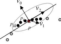
Suppose pi be a sampled point, N(pi) be it’s k-neighborhood(see fig.1), the covariance matrix is defined as
⎥
⎥
⎥
⎥
⎥
⎦
⎤
⎢
⎢
⎢
⎢
⎢
⎣
⎡
⎥
⎥
⎥
⎥
⎥
⎦
⎤
⎢
⎢
⎢
⎢
⎢
⎣
⎡
− − −
− − −
=
p p
p p
p p
p p
p p
p p C
ik i i T
ik i i
L L
2 1
2 1
, (8)
in which, pis the barycenter of N(pi),pij∈N(pi).
Let the three eigenvalues of C be λi(i =0,1,2) . Because the matrix C is positive and semi-definite,
0
≥
λi .Suppose λ0 ≤λ1 ≤λ2. The three eigenvectors respectively corresponding to λi are vi(i=0,1,2), which compose an orthogonal basis. Across barycenter ofN(pi), three planes are obtained with vias the normal. These three planes cross each other orthogonally. Let L be a plane(x− p)v=0across the barycenter p in which vis the unit normal vector. Then the sum of square distance from all points in N(pi) to the plane is
2 || ( )) || / || ||2 2 T ij
d =
∑
p −p v v =v Cv. (9)Let
0 0 1 1 2 2
v a v= +a v +a v . (10)
Then 2 T d =v Cv
0 0 1 1 2 2 0 0 1 1 2 2
(a v a v a v )TC a v( a v a v )
= + + + +
2 2 2
0 0 0 1 1 1 2 2 2
T T T
a v Cv a v Cv a v Cv
= + +
2 2 2
0 0 1 1 2 2
aλ a λ aλ
= + +
2 2 2
0 1 2 0
(a a a )λ
≥ + +
0
λ = . If L0 is the plane
0
(x p v− ) =0, (11)
Then the sum of square distance from all points in N(pi)
to the planeL0is least. Then L0 can be envisioned as the least square plane. L0 is taken as the tangent plane ofN(pi) and as the normal of L0.
The surface variance is defined as[16]
) /(
)
( λ0 λ0 λ1 λ2
σ pi = + + . (12)
Surface variance reflects the deviation degree of the points to the tangent plane. In the flat region, the points in
) (pi
N are close to the tangent planeL0, then σ(pi) is small. In the rough region, the points in N(pi) are
dispersive to the tangent planeL0, then σ(pi)is large. So
) (pi
σ is a good approximation of the curvature at
p
. Based on the analysis above, the nonuniform simplification method based on surface variance can be presented. The space partitioning method of K-D tree is adopted to partition the data space. After partitioning, the generated leaf nodes contain all the sampled points.Before simplifying, three thresholds, the lower boundary of the number of the points in a leaf node M, the upper boundary of the number of the points in a leaf node N and the upper boundary of the curvature U are selected. When partitioned, the data set of a father node is divided into two subsets by a plane crossing the barycenter of the node along one axis of the three axes. These two subsets have the almost same number of points. Each subset corresponds to one subnode. If the number of points sampled in a node is bigger than the threshold N, this means that the local neighborhood yet contains more points and needs to partition again. If the number of points sampled is smaller than the threshold M, this means that the local neighborhood already contains few points and doesn’t need to partition. If the number of points is bigger than the threshold M but smaller than N, the surface curvature σwill be calculated and compared with the threshold U to decide whether to partition or not. If σis bigger than U, this means that the local neighborhood is rougher and the sampling density should be increased. Then the partitioning operation will be continued on the node. Otherwise, the local neighborhood is flat and the 1
v
2
v
0
v
p i p ik p
partitioning operation stops. The node is taken as a leaf node. For every leaf node, the sampled points closest to the barycenter of the node will be selected to represent all the points in the local neighborhood.
C. Data segmentation
It’s obviously that equation (5) is a quadratic programming problem with 2n optimization variables, n
linear equations and 4n linear inequations. If the points set contains many samples, the regressing time is considerable. In order to reduce the learning time of SVM, we have to take an segmentation strategy to overcome it. We divide the sampled points into several subsets Sis which satisfy
i
S =S
U ,
φ =
≠ j j i
i S
S I . (13)
Then a training set and a testing set are created for every subsetSi . Training every training set, a support vector setSVi is brought out.
However, theSVi corresponding to every training set is independent due to the independence ofSi. The SVis don’t have the internal relationship as the support vectors of original data set. This results in the discontinuity on the borders of training sets. Then the surface reconstructed is cracked as displayed in fig.4 (b) and (e) which is not unexpected. Two technologies are used to increase the continuity of the regress function on the borders:
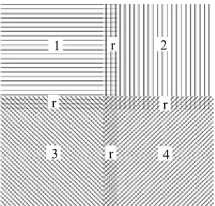
(1) making the adjacent data set share an overlapped region when segmenting(see fig.2);In other word words, if Si is adjacent to Sj, then letSiISj ≠φ.
(2) making the samples in the overlapped region have large weighting coefficients; this is to say, there have several copies of the kind of samples in the two subsets, so they are trained several times.
The first one makes the border an interior region of the training subset; the second one increases the weighting coefficients of points-sampled in shared region. These two technologies will improve the generalization of SVM on the borders.
Space partitioning scheme used surface variance[15] can be used to segment the points-sampled more uniformly. However, the high sampling density assumed in our data allows simple rectangle partitioning to work efficiently.
If the samples set S is divided into k subsets, the primal programming problem is transformed into
k quadratic programming problems. Suppose the computation complexity of every quadratic programming problem is O(nβ), then the total computation complexity after segmentation is ( β)/ β−1
k n
O . For classical quadratic
programming problem, β>2 , the total computation complexity after segmentation will be less than 1/k of the primal question. So, segmentation can reduce the computing consumption of regression theoretically.
D. The description of surface reconstruction based on SVM
The process of reconstruction based on SVM consists of two stages, training stage and testing stage. In the first stage, a SVM model consisting of all support vectors is acquired by training the training data set using the selected kernel function and training parameters. In the testing stage, testing output is gotten by testing the grid data using the SVM model.
Two methods can be used to construct the testing data. One is to construct according to the training data directly. By resampling the points, we can get a testing data set. The other is to construct by remeshing the training region. The second method can generate a mesh of the surface for scattered data. It is convenient for the following geometric processing. The second method is adopted to generate the testing data set.
The algorithm of surface reconstruction based on SVM is describes as the following steps:
(1) calculating the 2-dimension region of the samples, then divide the sampling data set into several subsets; any two adjacent subsets share a small strip region r.
(2) calculating a training data set Siand a testing data set according to every subset. Those points belonging to the shared region are appended into the adjacent training subsets for mtimes.
(3) training every Siusing selected kernel function and training parameters based on ε−SVM; and a SVM model will be created.
(4) testing on every testing data subset using the SVM model and generate a testing output.
(5) integrating all testing outputs into one mesh which represents the reconstructed surface.
Figure 2 Segmentation of training data
1 2
3 4
r
r r
III. EXPERIMENTS AND ANALYSIS
To verify the efficiency of our algorithms of simplification and segmentation surface reconstruction based on SVM, we experiment on a platform with Inter CoreII 2.13G/2G RAM/Geforce 8600GTS. The performance of our algorithm is measured by the quality of the final surfaces and the time consumption required to regress which are contrasted with the effect without segmentation.
A. Experiments
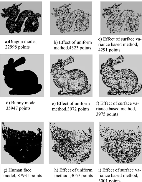
First, the cloud points is simplified using the method proposed in subsection B of section II. Three models are used to demonstrate the validity of the simplifying method. The simplifying result is shown in fig.3.
Thenε−SVM is adopted to regress surfaces with the Gauss kernel function.
) / || ||
exp( ) ,
(xi xj = − xi−xj 2 α2
k . (14)
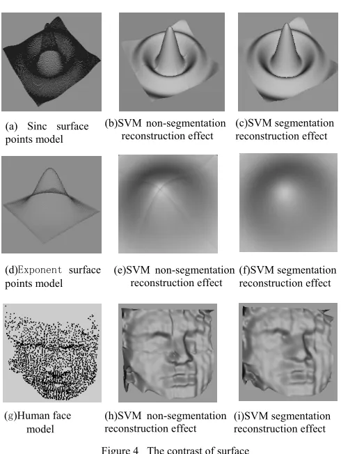
Three kinds of points set are selected to verify our segmentation recontruction method. Two of them are cloud points set created from sinc function surface function and exponent function surface. The number of the sampled points of sinc function surface is 22500 and the number of points of the exponent function is 9800. The third one is human face model generated from stero
matching technology. The surfaces reconstructed from the simplified points of reconstruction are shown in fig.4.
B. Parameter selection
The performance of the simplification is determined by the thresholds M、N and U. Let S be the simplifying ratio. Usually, we have M<S<N. Changing the thresholds M and N, the ratio is changed accordingly. For cloud points, selecting big M and N, the significant simplifying performance is achieved. Parameters M and N make the algorithm avoid the oversimplifying which may occur in[15]. The third parameter U influences the capability of detail-preserving of the algorithm presented. Two kinds of data set, bunny model data set and human face data set are selected to test the performance of this method. From fig.3 we can see that the details on the dragon model simplified using surface variance method are preserved better than those on the model simplified using uniform method. The effect is as same as that on the Bunny model. Then the surface variance based method can adapt the variance of curvature on the surface better than the uniform method.
Experimental results also show that simplification reduces the computing consumption of regression significantly. Before simplification, the regression process on face data set is very slow and almost endless. After simplification, the process is finished in tens of second with the same SVM parameters. This makes the reconstruction based on SVM practical.
A more important problem is the influence of the simplification to accuracy of reconstruction. We compare the testing result on the original sampled points using the SVM model by training the original sinc data set and the simplified sinc data set. The error of the first SVM model is about 174.2 and the error of the second SVM model is about 182.0. Then the error introduced by the simplification is about 4% of the whole error of the first SVM model. Therefore, in spite of the great simplifying ratio and the performance of regression, the accuracy of reconstruction doesn’t decline obviously. Fig.4 illustrates that smooth surfaces are achieved by the SVM based method. So, the SVM method keeps the smoothness of the models.
The segmentation parameters include the number of blocks k , the size of common region r and the parameterm. For parameterk, the bigger k is, the less the number of points in the subset is due to there are more common regions shared by some subsets. Because of the less points in every subset, the regression time of every subset deceases with the increasing ofk. But the total regression time behaviors different. When kis bigger than certain value, the total time consumed to regress will increase due to the points appended to the whole training data sets increasing as well as extra time consumption caused by segmenting. For the parameterr, the bigger r
is, the more continuous the reconstructed surface is. But the training data increases at the same time and consumes Figure 3 Effect of simplification
d) Bunny mode, 35947 points
g) Human face model, 87931 points
i) Effect of surface va- riance based method, 3001 points e) Effect of uniform
method,3972 points
f) Effect of surface va- riance based method, 3975 points
h) Effect of uniform method ,3057 points a)Dragon mode,
22998 points b) Effect of uniform method,4323 points
more training time. For parameterm, to increase mis to increase the punishing factors of the points located in the region in common. Therefore, the generalization is improved at the cost of more time consumption. Generally speaking, if the number of training data is more than 1000, the training speed will descend greatly. So the parametersk,rand mshould take the appropriate values. For our experiments, thek=4, r =1/20, m=2 can provide the expected effect. The reconstructed surface is continuous as well as the time consumption to regress is sound.
The main SVM regression parameters include punishing factor Cand training errorε. They determine the capability of generalization. If C is too big, the punishment on samples beyond the ε band is heavy, making the generalization bad although the training error is small. Otherwise, if Cis too small, the punishment on samples beyond the ε band is light, making the generalization good but the training error is large. To training errorε, if ε is too big, the training margin is large and the ε band is wide, then the regression accuracy is high but the number of SVi is increased. The expression (7) becomes complex. Otherwise, if ε is too small, the margin is small and the ε band is narrow, then the regression accuracy is low but the number of SVi
deceases. The expression (7) becomes simple. So the selection of C and ε is in a dilemma. There is no universal method for selecting of parameters C andε. We use the cross-validation technique to select parametersC and ε.
C. The effect of reconstruction
We selectk=4, and then the original sampled points set is divided into four subsets. The common region shared by several subsets is about 1/20 of the whole region and mequals 2. In order to explain the efficiency of our method, a contrast is made between segmentation reconstruction with a common region and segmentation reconstruction without a common region. The effect is shown in fig.4. From fig.4 (b), (e)and (h), (c), (f)and (i) we can see that if the subsets share no common region, the surface integrated from subsurfaces is cracked and discontinuous. Then the continuity of the original surface is damaged. Using the method of segmentation reconstruction proposed in this paper, the surface integrated from subsurfaces is continuous even on the borders. The continuity of the model is kept down. It is obvious that the second method is better than the first. Consider the smoothness, fig.4 (c) and (f) also show that if the primal configuration is smooth, the second method will keep the smoothness of the surface. This demonstrates that SVM regression has the excellent capability of function approximate.
D. Efficiency analysis
Although the segmentation reconstruction method decreases the complexity of the programming problem, it also increases the number of training data which can degree the efficiency of the method. The number of samples appended is about 10% of the original points set. Select appropriate SVM parameters to compare the performance improved. The table 1 shows the performance of segmentation reconstruction. Generally speaking, the segmentation method will decrease the regression time to more than a half of the unsegmentation method.
Although existing 10% common region, the training time consumed deceases obviously after segmentation. The time consumed of segmentation is 1/5 of non-segmentation. As k equaling 4, it accords with the analysis in section II. So the algorithm proposed in this paper is very efficient.
Table 1 The efficiency of segmentation regression
Models Time consumption of non-segmentation Time consumption of segmentation
Sinc surface 21s 5.3s
Exponent surface 51s 24.7s
Human face 464s 91s
(g)Human face model (a) Sinc surface points model
(b)SVM non-segmentation reconstruction effect
Figure 4 The contrast of surface reconstruction based on SVM
(c)SVM segmentation reconstruction effect
(h)SVM non-segmentation
reconstruction effect (i)SVM segmentation reconstruction effect (e)SVM non-segmentation
reconstruction effect (d)Exponent surface
points model
IV. CONCLUSION
Surface reconstruction is an important topic in reverse-engineering and applications of virtual environment reconstruction. The simplification method and regression algorithm are researched in this paper. A simplification method based on surface variance using K-D partitioning technique is presented. A segmentation regression strategy based on ε−SVM is studied by which the sampling data are divided into several subsets. Then SVM regression is executed on the subsets rapidly. The complexity of the problem is descended and the time consumption is reduced obviously. Experiments prove the efficiency of this algorithm.
ACKNOWLEDGEMENT
This research is partially funded by the National HighTech Research and Development Plan of China under Grant No. 2006AA0517. The authors thank to Dr. Tao Wu and Tingbo Hu for providing the human face data used in this paper. Our thanks also to Stanford University for making these models available to us.
REFERENCES
[1] H. Hoppe, T. DeRose, T. Duchamp, et al, “Surface reconstruction from unorganized points,” Computer Graphics, 1992, v26, n2, pp71-78.
[2] J.J. Wu, Q.f. Wang, Y.B.o Huang, et al, “Review of surface reconstruction methods in reverse engineering,” Journal of Engineering Graphics, 2004, 25(2):133-142.
[3] J. Stiller, “Point-normal interpolation schemes reproducing spheres cylinders and cones,” Geometric Design, 2007, v24, n5, pp286-301.
[4] J. Peters, “Local smooth surface interpolation: a classification,” Computer Aided Geometric Design, 1990, v7, n1-4, pp191-195.
[5] Y.b.Wang, Y.h Sheng., G.n Lv., et al, “A Delaunay-based Surface Reconstrution Algrithm for Unorganized Sampling Points,” Journal of Image and Graphics, 2007, v12, n9, pp1537-1543.
[6] J.G. Li, D, Yang, X.H. Meng, Q.M. Chen, et al, “Conforming Voronoi Tessellation in 3D,” Journal of Computer-Aided Design&Computer Graphics, 2005, v17, n10, 2143-2151. [7] X.Y. Zhang, S.Y. Zhang, X.Z. Ye, “Interactive free-from
deformation for sculpture,” Journal of Computer-Aided Design&Computer Graphics, 2005, v17, n11, 2420-2426. [8] J.V. Miller, D.E. Breen, W.E. Lorensen, et al,
“Geometrically deformed models: a method for extracting closed geometric models from volume data,” SIGGRAPH’91, 1991, v25, n4, pp217-226.
[9] G. Turk, J.F. O’Brien, “Shape transformation using variational implicit functions,” SIGGRAPH’99, 1999, pp335-342.
[10] P. Gu, X. Yan, “Neural network approach to reconstruction of freeform surfaces for reverse engineering,” Computer Aided Design, 1995, v27, n1, pp59-64.
[11] H.T. Wang, L.Y. Zhang, Z.W. Li, et al, “B-spline surface reconstruction from scattered data points based on SOM neural network,” Journal of Image and Graphics, 2007, v12, n2, pp349-355.
[12] V. N. Vapnik, “The nature of statistical learning theory,” Springer Verlag, New York,1995.
[13] B. Scholkopf, J. Giesen, S. Spalinger, “Kernel methods for implicit surface modeling,” Technical Report,
ftp://ftp.kyb.tuebingen.mpg.de, 2004.
[14] Y.Cai, J.Xiao, “Surface reconstruction from points based on support vector machine,” Journal of System Simulation, 2007, v19, n15, pp2027-2029.
[15] H.T.Wang, L.Y.Zhang, J.Du, et al, “Simplification and error analysis based on implicit surface for measuring points-sets,” Journal of Image and Graphics, 2007, v12, n11, pp2114-2118.
[16] M. Pauly, L. Kobbelt, M. Gross, “Multiresolution modeling of point-sampled geometry,” Technical Report vol.378, ETH Zurich: Institute of Scientific Computing, 2002. [17] D. J. Weir, M.J. Milroy, C. Bradley, et al, “Reverse
engineering physical models employing wrap-around B-spline surfaces and quadrics,” Journal of Engineering Manufacture-Part B, 1996, 210, pp147-157.
[18] L.Ma, G.h.Peng, D.f.Geng, “Nonuniform simplification of cloud data based on octree,” Computer Application, 2007,v27, n8, pp3614-3618.
[19] M.Desbrun, M. Meyer, P. Schroder, et al. “Implicit fairing of irregular meshes using diffusion and curvature flow,” SIGGRAPH’99, 1999, pp317–324.