Runway Incursion Event Forecast Model based on LS-SVR with Multi-kernel

Runway Incursion Event Forecast Model based

on LS-SVR with Multi-kernel

Guimei Xu1_{, Shengguo Huang}2 College of Civil Aviation,

Nanjing University of Aeronautics and Astronautics, Nanjing, China

Email: 1_{[email protected],} 2_{[email protected]}

Abstract—Forecasting of runway incursion event is very significant to guide the job of civil aviation safety management. It is an important part of the runway incursion early warning management. However, prediction of runway incursion event is a complicated problem due to its non-linearity and the small quantity of training data. As a novel type of learning machine, support vector machine (SVM) has been gaining popularity due to their promising performance, such as dealing with the data of small sample, the high dimension and the excellent generalization ability. However, the generalization ability of SVM often relies on whether the selected kernel function is suitable for real data. To lessen the sensitivity of different kernels and improve generalization ability, least square support vector regression (LS-SVR) with multi-kernel is proposed to forecast the runway incursion event in this paper. The two experimental results indicate that LS-SVR with multi-kernel model is better than LS-SVR with individual kernel model and generalized regression neural network (GRNN) model. Consequently, multi-kernel LS-SVR model is a proper alternative for forecasting of the runway incursion event.

Index Terms—airport runways; forecast model; least square support vector machine; multi-kernel

I. INTRODUCTION

Runway incursion is a kind of unsafe event, which seriously affect airport safety. It is easy to cause disastrous collision or accident. Recently, under the request of international civil aviation organization (ICAO), the various countries begin to solve the problem of runway incursion vigorously [1, 2].Civil aviation administration of China brings this question into the project of the national 863 plans “a new generation national of air traffic management system”, and starts implementing the project of “civil aviation airport runway safety programming” in 2008. Therefore, runway incursion event has already become the hot spot research in civil aviation. Forecasting runway incursion event exactly can provide reliable basis for training people and working out flight plan scientifically, guide the job of civil aviation safety management and prevent runway incursion event occurring.

At present, artificial neural network (ANN) is a

popular tool to research the nonlinear system [3, 4]. The theory foundation of artificial neural network algorithm is based on traditional statistics, consequently, ANN need a large amount of training data. However, runway incursion is small probability event and its data is generally little. Therefore, ANN is not suitable for forecasting of runway incursion event. Superior forecasting accuracy can be gained with a small quantity of training data by grey model, but grey model only depicts a monotonously increasing or decreasing process with time as exponential law. So a certain error is always generated in forecasting runway incursion event by using grey model. Therefore, it is imperative to look for a more excellent method in forecasting runway incursion event.

Developed by Vapnik [5，6], SVM is the method which is receiving increasing attention with remarkable results recently. The main difference between ANN and SVM is the principle of risk minimization. ANN implements the empirical risk minimization principle to minimize the error on the training data. However, SVM implements the principle of structural risk minimization in place of experiential risk minimization, which makes it has excellent generalization ability in the situation of small sample. In addition, SVM can change a non-linear learning problem into a linear learning problem in order to reduce the algorithm complexity through kernel trick, which allows every dot product to be replaced simply by a kernel function. Different kernel functions can be chosen during the SVM regression, corresponding to the different transformed feature spaces. So kernel functions play an essential role in the SVM regression since they determine the feature spaces in which data examples are fitted and can directly affect the SVM regression results and performances.

When applying SVM to solve real regression problems, one has to deal with the practical difficulty: how to select an appropriate kernel function which fits particular data better than any other kernel functions. An abnormal way is to try many different kernels and choose the one which works best. But this approach could be time-consuming if the size or the number of attributes of training data is huge. In this paper, multi-kernel SVM in which several different kernels are combined is been put forward. The SVM with multi-kernel model is probably expected to outperform the SVM with individual kernel model because different kernels might complement each other well. SVM regression is defined as support vector

This work was supported by the National Natural Science Foundation of China (Grant No. 60879008).

regression (SVR). LS-SVR algorithm is improved based on SVR algorithm. Therefore, LS-SVR with multi-kernel model is used to forecast runway incursion event in this study. At last, the LS-SVR with multi-kernel is compared to GRNN and LS-SVR individual kernel.

The organization of the paper is as follows. We will review the theories of SVR and LS-SVR in Section II. In Section III, we will introduce multi-kernel LS-SVR algorithm. Multi-kernel LS-SVR model and parameters optimization algorithm will be introduced in Section IV. In Section V and VI, we will present the two experiments and results. Finally, conclusions are drawn in Section VII.

II. ARITHMETIC OF SVR AND LS-SVR A. SVR Algorithm

Recently, SVM has been applied successfully to solve non-linear regression estimation problems [7-11]. A regression version of SVM has emerged as an alternative and powerful technique to solve regression problems by introducing an alternative loss function. In the sequel, this version is referred to as support vector regression (SVR). Here a brief description of SVR is given.

Given a set of data

( , )

x y

i i ,

d i

x

∈

R

，

(

1, 2,..., )

i

y

∈

R i

=

n

，where

x

_i denotes the input vector,

y

_idenotes the corresponding output value and

n

denotes the total number. In SVR, the regression function is approximated by the following function:

1

1 2 1 2

( )

( )

[ ,

,...,

] ,

[ , ,..., ]

h

T i i

i

T T

h h

y

w

x

b

W

x

b

W

w w

w

φ

φ

φ φ φ

φ

=

=

+ =

+

=

=

∑

₍₁₎

Where,

b

is the scalar threshold,

W

is the weight coefficient, and

φ

( )

x

is called the feature nonlinearly mapped from the input space

x

.

The above problem is equivalent to the solution of the following optimal problem:

1

min

2

( )

. .

1, 2,...,

( )

T T

i i

T

i i

J

W W

y

W

x

b

s t

i

n

W

x

b

y

φ

ε

φ

ε

=

⎧ −

− ≤

⎪

₌

⎨

+ − ≤

⎪⎩

(2)

Sometimes, the optimal solutions can not be obtained form above equations. We introduce slack variables

ξ

,

ξ

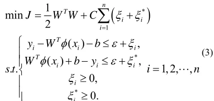
* to guarantee that the convex optimization problem is feasible. Hence the optimization problem is expressed as:

(

*

)

1

*

*

1

min

2

( )

,

( )

,

. .

1, 2, ,

0,

0.

n T

i i i

T

i i i

T

i i i

i i

J

W W

C

y

W

x

b

W

x

b

y

s t

i

n

ξ ξ

φ

ε ξ

φ

ε ξ

ξ

ξ

=

=

+

+

⎧ −

− ≤ +

⎪

_{+ − ≤ +}

⎪

₌

_⋅⋅⋅

⎨

_≥

⎪

⎪

_≥

⎩

∑

(3)

The constant C (C>0) determines the tradeoff between flatness of f and the amount of tolerable deviations which are larger than

ε

. The formulation above corresponds to the solution of a loss function described by:

| | :

0

| |

,

| |

.

if

otherwise

ε

ξ ε

ξ

ξ ε

≤

⎧

= ⎨

₋

⎩

(4)

The loss function is shown in Fig.1.

Figure 1. The soft margin loss setting for a linear SVR

Finally, by introducing Lagrange multipliers and kernel function, and maximizing the dual function of Eq. (3), the regression function given by Eq. (1) has the following explicit form:

*

1

( )

(

) ( , )

n

i i i

i

f x

a

a K x x

b

=

=

∑

−

+

(5)

In Eq. (5),

a

_i and

a

*_i are the so-called Lagrange multipliers. They satisfy the equalities

a

i

×

a

i*

=

0

,

0

i

x

≥

and

a

_i*

≥

0

where

i

=

1, 2,...,

n

, and are obtained by maximizing the dual function of Eq. (3), and the maximal dual function in Eq. (3) which has the following form:

* * *

1 1

* * 1 1

( , )

(

)

(

)

1

(

)(

) ( , )

2

n n

i i i i i i i

i i

n n

i i j j i j i j

Max R a a

y a

a

a

a

a

a

a

a K x x

ε

= =

= =

=

−

−

+

−

−

−

∑

∑

∑∑

(6)

* 1

*

(

) 0,

0

1, 2,..., ,

0

1, 2,..., .

n

i i i

i i

a

a

a

C

i

n

a

C

i

n

=

−

=

≤ ≤

=

≤

≤

=

∑

(7)

Based on the Karush — Kuhn — Tucker’s (KKT) conditions of solving quadratic programming problem, (

a

_i

−

a

_i*) in Eq. (5), only some of them will be held as non-zero values. These approximation errors of data point on non-zero coefficient will equal to or larger than

ε

, and are referred to as the support vector. That is, these data points lie on or outside the

ε

-bound of decision function. According to Eq. (5), the support vectors are clearly the only elements of the data points employed in determining the decision function as the coefficient

a

_i

−

a

*_i of other data points are all equal to zero. Generally, the larger the

ε

value, the fewer the number of support vectors, and thus the sparser the representation of the solution. Nevertheless, increasing

ε

decreased the approximation accuracy of training data. In this sense,

ε

determines the trade-off between the sparseness of representation and closeness to data.

The term

K x x

( , )

_{i j} in Eq. (5) is called the kernel function. Where the value of kernel function equals the inner product of two vectors

x

_i and

x

_j in the feature space

φ

( )

x

_i and

φ

( )

x

j , meaning that

( , )

_{i j}

( )

_i

( )

_j

K x x

=

φ

x

•

φ

x

. The kernel function is intended to handle any dimension feature space without the need to calculate

φ

( )

x

accurately [12]. If any function can satisfy Mercer’s condition, it can be employed as a kernel function [6]. In SVR, several kernel functions have been used widely and successfully, such as polynomial basis function with degree d

( , ) (

T

1) ,

d

1, 2,...

i j i i

K x y

=

x y

+

d

=

(8) Gaussian RBF kernel with tuning parameter σ，

K x x

( , ) exp(

i j

=

−

&

x

i

−

x

j

&

2

/2

σ

2

)

(9)

and sigmoid function with parameterθ,

K x y

( , ) tanh(

i j

=

x x

i

⋅ −

j

θ

)

(10)

B. LS-SVR Algorithm

LS-SVR tries to minimize primal cost function subject to equality constraints instead of inequality ones. Therefore, LS-SVR solves a set of linear equations instead of computational cost quadratic programming problem. According to statistics theory and abnormal SVR knowledge, the training sample regression problem can be described into the Eq. (1).

According to structural risk minimization, through transforming error’s first power to two powers, the sample regression problem can be described into the following restraint optimization problem:

2 1 ,

1

1

min ( , )

2

2

. .

( )

1, 2,..., .

n T

i i T

i i i

J W e

W W

C

e

s t

y

W

φ

x

b e

i

n

=

=

+

=

+ +

=

∑

₍₁₁₎

Where, ei∈R denotes slack variables, J denotes loss function, C is a regularization parameter.

By transforming this formula into dual form with Lagrange multipliers ai, following formula is obtained.

1

( , , ; )

( , )

{

( )

}.

n

T

i i i i

i

L W b e a

J W e

a W

φ

x

b e

y

=

=

−

∑

+ + −

(12)

Based on the Karush-Kuhn-Tucker’s (KKT) conditions:

1

1

0

( )

0

0

0

0

( )

0

n i i i

n i i

i i i

T

i i i

i

L

W

a

x

W

L

a

b

L

a

Ce

e

L

W

x

b e

y

a

φ

φ

=

=

∂

= →

=

∂

∂

_{= →}

₌

∂

∂

_{= → =}

∂

∂

_{= →}

_{+ + − =}

∂

∑

∑

(13)

From equation set above, W and e can be eliminated.

0

₁

0

T

b

I

a

y

I

C I

−

⎡

⎤ ⎡ ⎤ ⎡ ⎤

=

⎢

_{Ω +}

⎥ ⎢ ⎥ ⎢ ⎥

⎣ ⎦ ⎣ ⎦

⎣

⎦

(14)

Where, a = [a1, a2… al]; Ωij = K(xi, xj) = Φ(xi)TΦ(xj). The solution of ai and b can be obtained. Hence, the LS-SVR decision function is:

1

( )

( , )

n

i i i

y x

a K x x

b

=

=

∑

+

(15)

III. MULTI-KERNEL LS-SVRALTORITHM

Eq. (15) is the decision function of LS-SVR with individual kernel. It has the following limitations [13, 14]: first, this decision function can only correspond to some special function sets, but it can not correspond to some mixed function sets. For example, if kernel function is RBF function, then the decision function correspond to some radial basis function sets, not mixed function sets of radial basis function and polynomial function. Second, the majority of kernel functions have a free parameter to control its generalization performance (for example, RBF kernel with σ parameter). This individual kernel function can not select several free parameters. Therefore, based on abnormal LS-SVR algorithm, multi-kernel LS-SVR algorithm is presented.

1 r T k k k

y

W

φ

b

=

=

∑

+

(16)

Where,

[

₁

,

₂

,...,

]

T k k k kh

W

=

W W

W

, r is the number of

select kernel functions.

Optimization objective function is:

2

1 1

1

1

1

min ( , )

2

2

. .

( )

,

1, 2,..., .

r n

T

k k k i

k i

r T

i k k i i

k

J W e

C W W

C

e

s t y

W

φ

x

b e i

n

= =

=

=

+

=

+ +

=

∑

∑

∑

(17)

Where,

C k

_k

,

=

1, 2,...,

r

are penalty factors of kernel functions.

Lagrange function is:

1 1

(

, , , )

( , )

{

( )

}

k i i

n r

T

i k k i i i

i k

L W b e a

J W e

a

W

φ

x

b e

y

= =

=

−

+ + −

∑ ∑

(18)

Based on KKT conditions, Eq. (13) becomes:

1

1

1

1

0

( )

0

0

0

0

( )

0

n

k i k i i k k n i i i i i r T

k k i i i k

i

L

W

a

x

W

C

L

a

b

L

a

Ce

e

L

W

x

b e

y

a

φ

φ

= = =

∂

= →

=

∂

∂

= →

=

∂

∂

_{= → =}

∂

∂

_{= →}

_{+ + − =}

∂

∑

∑

∑

(19)

From equation set above,

W

_k and

e

_i can be eliminated.

0

_{' 1}

0

T

b

I

a

y

I

C I

−

⎡

⎤ ⎡ ⎤ ⎡ ⎤

=

⎢

_{Ω +}

⎥ ⎢ ⎥ ⎢ ⎥

⎣ ⎦ ⎣ ⎦

⎣

⎦

(20)

Where, ' 1 1

1

1

( ), ( )

( , )

r r

ij i j k i j

k k k k

x

x

K x x

C

φ

φ

C

= =

Ω =

∑

<

> =

∑

The multi-kernel LS-SVR decision function is:

1 2 1 2 1

( , )

( , )

( )

( , )

n

i i i i

r

i _{i r i}

a K x x

a K x x

y x

a K x x

b

=

+

+

=

+

+

∑

"

(21)

Where, j i

a

denote the weight of the jth kernel function correspond to the ith training sample.

1

,

2

,

r

K K

"

K

denote different kernel functions. IV. MULTI-KERNEL LS-SVRMODEL IN FORECASTING

THE RUNWAY INCURSION NEVENT

Forecasting of runway incursion event is the time series forecasting problem. And the goal is to search a forecasting model with excellent generalization ability by utilizing the training sample obtained by historical data.

The process of constructing multi-kernel LS-SVR model is described below.

A. Construction of Training Sample Sets

For a time series An= {a1, a2, …, an}, training sample sets T= {(x1, y1), …, (xn-m, yn-m)} are established. Where

1 2 1

2 3 1 2

1 1

,

m m

m m

n m n m n n

a

a

a

a

a

a

a

a

X

Y

a

a

a

a

+ + + − − + −

⎡

⎤

⎡

⎤

⎢

⎥

⎢

⎥

⎢

⎥

⎢

⎥

=

=

⎢

⎥

⎢

⎥

⎢

⎥

⎢

⎥

⎣

⎦

⎣

⎦

"

"

#

#

#

#

#

"

(22)

xi={ai,ai+1,…,ai+m-1} is the input vector, yi={ai+m} is the output value, m is the embedded dimension.

B. Optimizing Parameters of the Multi-kernel LS-SVR Model

Despite its superior features, LS-SVR is limited in academic research and industrial applications, because the user must define various parameters appropriately. To construct the LS-SVR model efficiently, LS-SVR’s parameters must be set carefully [14, 15]. Inappropriate parameters in LS-SVR lead to over-fitting or under-fitting. Different parameter settings can cause significant differences in performance. Therefore, selecting the optimal hyper-parameter is an important step in multi-kernel LS-SVR model design. The parameters include:

(1) Kernel function: The kernel function is used to construct a nonlinear decision hyper-surface on the LS-SVR input space. In this paper, Polynomial basis function with d and Gaussian RBF function with tuning parameter

σ

₁ and

σ

₂ are selected as kernel functions.

(2) Regularization parameter C: C determines the trade-off

cost between minimizing the training error and minimizing the model’s complexity.

Multi-kernel LS-SVR model generalization performance (estimation accuracy) and efficiency depends on the

hyper-parameters (C, d,

σ

₁ and

σ

₂) being set correctly.

Therefore, following discuss the step of parameters optimization.

Step 1: sketchy initialization

C

and

d

are

C

′

and

d

′

.

Step 2: set

C

=

C

′

and

d

=

d

′

, seeks for a group superior

σ

₁* and

σ

*₂.

Step 3: set

σ

₁

=

σ

₁* and

σ

₂

=

σ

₂*, seeks for a group

superior

C

*and

d

*.

V. ONE EXPERIMENTAL ANALYSIS A. Selection of Sample Data

B. Determination of the Embedded Dimension m

The election of embedded dimension m has a great influence on the forecasting performance of LS-SVR. Sample data are used to test the effect of embedded dimension m on forecasting accuracy.

In this study, root mean square relative error (RMSRE) is used as the performance index, which is as follows:

2

1

ˆ

1

(

)

100%

l

i i i i

y

y

RMSRE

l

=

y

−

=

∑

×

(23)

Where y_i and yˆ_i represent the actual and validation values respectively, l is the number of testing samples.

RMSRE values of testing data gained by LS-SVR which trained with various m values are shown in Fig.2, It indicates that the election of embedded dimension m has a great influence on the forecasting accuracy.

Figure 2. Effect of embedded dimension m on forecasting accuracy

As shown in Fig.2, when m=5, RMSRE achieves the minimum value. Therefore, in this study, take m=5 as the optimal embedded dimension.

C. Optimizing the Model Parameters

The process of parameters optimization is shown in TABLE I and II. Where, “*” values denote the superior parameters.

TABLEI. SELECTION PROCEDURE OF

σ

₁ AND

σ

₂ WHILE C=1, d=3.

1

σ

σ

₂ RMSRE

0.01 1000 0.221

0.1 1000 0.214

1 1000 0.212

10* 1000* 0.141*

100 1000 0.189

10 0.01 0.256

10 0.1 0.213

10* 1* 0.089*

10 10 0.197

10 100 0.263

TABLE II. SELECTION PROCEDURE OF C AND d WHILE 1

10

σ

=

AND

σ

₂

=

1

.

C d RMSRE

0.01 1 0.136

0.1 2 0.093

1 3 0.089

10* 4* 0.036*

100 5 0.104

According to TABLE I and II,

* * * *

1 2

10,

4,

10,

1.

C

=

d

=

σ

=

σ

=

D. Analysis the Results of Forecasting Model

Using the parameters of m, C, d,

σ

₁ and

σ

₂ which were determined above to train the multi-kernel LS-SVR model. The regression model is achieved. The regression curve of runway incursion event is shown in Fig.3.

Figure 3. Regression curve of runway incursion event

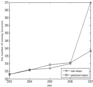
As shown in Fig.3, the LS-SVR with multi-kernel model exactly depicts the distributing of the sample data. Using the model to predict the number of runway incursion event from 2003 to 2007, then testing curve is shown in Fig.4.

As shown in Fig.4, the LS-SVR with multi-kernel model basically forecast the tendency of runway incursion event from 2003 to 2007. Although the

difference between real value and predicted value of the certain spot is big, but the overall change tendencies of two curves are consistent.

TALBE III. TRAINING PERFORMANCE OF THREE MODELS

MKLS-SVR LS-SVR GRNN

year real value predicted value predicted value predicted value

1993 186 186.025 186.153 187.089

1994 200 200.023 200.987 201.456

1995 240 239.956 239.023 238.458

1996 275 275.031 275.631 276.542

1997 292 292.142 292.753 293.980

1998 325 325.027 325.346 326.273

1999 327 327.145 327.360 328.781

2000 405 405.070 405.321 407.046

2001 407 407.324 408.163 410.683

2002 339 339.056 339.793 340.056

MAE 0.089 0.649 1.745

RMSE 0.126 0.725 1.888

TALBE IV. PREDICTION PERFORMANCE OF THREE MODELS

MKLS-SVR LS-SVR GRNN

year real value predicted value predicted value predicted value

2003 323 323.039 323.142 323.864

2004 326 325.895 325.670 324.888

2005 327 328.227 328.615 329.487

2006 330 330.670 331.621 332.005

2007 370 338.330 336.210 331.245

MAE 6.742 7.500 9.045

RMSE 14.177 15.147 17.402

In order to analysis the performance of the LS-SVR with multi-kernel (MKLS-SVR) model, the LS-SVR with individual kernel (LS-SVR) model and GRNN model are established at the same time. Mean absolute error (MAE) and root mean square error (RMSE) are used to evaluate the training and forecasting accuracy of the three models. The training and forecasting results of three models are shown in TABLE III and IV. As shown in TABLE III and IV, MAE and RMSE of multi-kernel LS-SVR model are smaller than the other models. It indicates: in the aspect of training and forecasting performance, LS-SVR model has better training and forecasting ability than GRNN model; in the aspect of kernel function, multi-kernel function is better than individual function.

VI. ANOTHER EXPERIMENTAL ANALYSIS A. Selection of Sample Data and Parameters

The sample data is the same of the above experiment. The regularization parameter C of LS-SVR is set 1 during the LS-SVR training. The two kinds of kernels: polynomial kernels and RBF kernels are selected to train the data. The degree of the polynomial kernels is set to 1, 2, 3, 4, 5 and the parameter

σ

of the RBF kernels is set to 0.001, 0.01, 0.1, 1, and 10. TABLE V shows the forecasting accuracies of the sample dataset. Next, we select three kernels randomly which ensemble multi-kernel LS-SVR to obtain the forecasting accuracies, as show in TABLE VI.

TABLE V. FORECASTING ACCURACIES OF SEVERAL KERNEL FUNCTIONS

Poly_kernel d RMSRE RBF_kernel σ RMSRE

Poly_1 1 0.138 rbf_0.001 0.001 0.054

Poly_2 2 0.068 rbf_0.01 0.01 0.052

Poly_3 3 0.061 rbf_0.1 0.1 0.049

Poly_4 4 0.068 rbf_1 1 0.046

TABLE VI. FORECASTING ACCURACIES OF THREE SELECTED KERNEL FUNCTIONS

Forecast RMSRE RMSRE RMSRE Average MKLS-SVR 1 Poly_1 0.138 Poly_2 0.068 rbf_0.01 0.052 0.086 0.048 2 Poly_1 0.138 Poly_3 0.061 rbf_0.1 0.049 0.083 0.046 3 Poly_4 0.068 rbf_1 0.046 rbf_0.01 0.052 0.055 0.043 4 Poly_1 0.138 Poly_3 0.061 Poly_5 0.080 0.093 0.064 5 rbf_0.1 0.049 rbf_1 0.046 rbf_10 0.043 0.046 0.044 B. Performance Analysis

The following gives the detailed analysis about the experimental results from the multi-kernel LS-SVR model.

In three of the five forecasts (forecasts 1-3), the multi-kernel LS-SVR model outperforms the best LS-SVR with individual kernel function model. Even if one or two of the three LS-SVR with individual kernel model have big RMSRE (0.138), the multi-kernel LS-SVR model can still achieve small RMSRE (0.049). For example, in forecast 2, the forecasting RMSRE of the three LS-SVR with individual model are 0.138, 0.061 and 0.049, while the RMSRE from the multi-kernel LS-SVR is 0.046. This is a good example to demonstrate that different kernel functions can complement each other in the multi-kernel LS-SVR model to achieve a better performance than any of the LS-SVR with individual kernel. In forecast 4 and 5, the multi-kernel LS-SVR model does not beat the best of the LS-SVR with individual model though it achieves better performance than the average and the second best. The possible reason is that in either of the forecasts, the two multi-kernel LS-SVR models have the same type of the kernel function but different parameters of the kernels. The two multi-kernel LS-SVR models with the same kernel type may work similarly for the same data and do not have too much information to complement.

VII. CONCLUSION

In this paper, multi-kernel LS-SVR model is applied to forecast runway incursion event. The real data sets are used to investigate its feasibility in forecasting runway incursion. LS-SVR implements the principle of structural risk minimization in place of experiential risk minimization, which makes it have excellent generalization ability in the situation of small sample. In addition, multi-kernel LS-SVR model is suitable for forecasting runway incursion event, which different kernel functions can complement each other well. The two experimental results reveal the potential of the proposed approach for forecasting runway incursion event.

REFERENCES

[1] Transport Canada, “National Civil Aviation Safety

Committee Sub-Committee on Runway Incursions,” Final Report, pp.7-12, Sep.2000.

[2] FAA, “FAA Runway Safety Report,” Jue.2003.

[3] J. W. Taylr, R. Buizza, “Neural network load forecasting

with weather ensemble predictions,” IEEE Transactions

on Power Systems, Vol.17, No.3, pp.626-632, 2002.

[4] E. Jorjani, S. C. Chelgani, S. Mesroghli, “Application of

artificial neural network to predict chemical

desulfurization of Tabas coal.” Fuel, Vol.87, No.12,

pp.2727-2734, 2008.

[5] V. N. Vapnik, “Estimation of Dependencies Based on

Empirical Data,” Berlin: Springer-Verlag, 1982.

[6] V. N. Vapnik, “The Nature of Statistical Learning Theory,”

New York: Springer-Verlag, 1995.

[7] J. T. Suykens, G. I. Van, “Least squares support vector

machines,” Singapore: Singapore World Scientific,

pp.13-15, 2002.

[8] C. H. Wu, T. Zeng, H. Wang, et al, “A real-valued genetic

algorithm to optimize the parameters of support vector

machine for predicting bankruptcy,” Expert Systems with

Applications, Vol.32, No.2, pp.397-408, 2007.

[9] P. F. Pai, “System reliability forecasting by support vector

machines with genetic algorithm,” Mathematical and

Computer Modeling, Vol.4, No.3, pp.262-274, 2006.

[10]K. Y. Chen, C. H. Wang, “Support vector regression with

genetic algorithms in forecasting tourism demand,”

Tourism Management, Vol.28, pp.215-226, 2007.

[11]B. Liu, H. Su, W. Huang, et al, “Temperature prediction

control based on least squares support vector machines,”

Journal of Control Theory and Application, Vol.4,

pp.365-370, 2004.

[12]F. E. H. Tay, L. Cao, “Application of support vector

machines in financial time series forecasting,” Omega,

Vol.29, No.4, pp.309-317, 2001.

[13]Z. J. Bao, D. Y. Pi, Y. X. Sun, “Nonlinear Model

Predictive Control Based on Support Vector Machine with

Multi-kernel,” Systems Engineering and Electronics,

Vol.15, No.5, pp.691-697, 2007.

[14]N. Zhang, Q. M. Liao, R. Su, et al, “Multi-kernel SVM

Based Classification for Tumor Segmentation by Fusion of

MRI Images,” International Workshop on Imaging

Systems and Techniques, pp.278-282, May.2009.

Guimei Xu was born in Jiangyan, Jiangsu province, China in

1980. She obtained a Bachelor degree in Computer Science and Technology from Nanjing University of Aeronautics and Astronautics, Nanjing, China in 2004.

She is currently a candidate for doctor’s degree of Nanjing University of Aeronautics and Astronautics, Nanjing, China. Her research interests include safety system engineering.

Shengguo Huang was born in Le-an, Jiangxi province, China in 1941. He obtained a Bachelor degree in control theory and application from Nanjing University of Aeronautics and Astronautics, Nanjing, China in 1965.