Half-Against-Half Structure with SVM and
k
-NN Classifiers in Benthic Macroinvertebrate
Image Classification
Henry Joutsijoki
School of Information Sciences, University of Tampere, Kanslerinrinne 1, FI-33014, Tampere, Finland Email: [email protected]
Abstract— We investigated how Half-Against-Half Support Vector Machine (HAH-SVM) and Half-Against-Half k -Nearest Neighbour (HAH-KNN) methods succeed in the classification of the benthic macroinvertebrate images. Au-tomated taxa identification of benthic macroinvertebrates is a slightly researched area and in this paper HAH-KNN was for the first time applied to this application area. The main problem, when Half-Against-Half structure is used, is to find the right way to divide the classes in nodes. This problem was solved by using two different approaches. Firstly, we applied the Scatter method for the class division problem. Secondly, we formed the class divisions in a Half-Against-Half structure by a random choice. We performed extensive experimental tests with four different feature sets and tested every feature set with seven different kernel functions in the case of SVM. Furthermore, HAH-KNN was tested with four measures. The tests showed that by the Scatter method and random choice formed HAH-SVMs performed the classification problem very well obtaining over 95% accuracy while with HAH-KNN above 92% accuracy was achieved. Moreover, the 7D and 15D feature sets together with the RBF kernel function are good choices for this classification task when HAH-SVM was used and 15D feature set, when HAH-KNN was used. Generally speaking, Half-Against-Half structure is a promising multi-class extension for SVM and an interesting variant fork-NN classifier.
Index Terms— benthic macroinvertebrates, support vector machine, k-nearest neighbour, half-against-half structure, classification
I. INTRODUCTION
The growing interest towards biological issues in the past decades has increased our knowledge about the nature and the environment surrounding us. The interest is still expanding and the exponentially growing amount of information brings us continuously more challenges to develop computationally better and more reliable tools for analyzing the data. Due to the nature’s diversity and, hence, its complexity general tools are difficult to invent. An important part of the nature is freshwater ecosys-tems. These are in a minority position when taking account into all aquatic environments in the Globe and, that is why, the constant biomonitoring is needed. Due to the environmental legislation, the need of biomoni-toring has increased in the past decades [26]. Benthic
This work was supported by Tampere Doctoral Program in Informa-tion Sciences and Engineering and with the grant given by Maj and Tor Nessling Foundation.
macroinvertebrates are an essential part of the freshwater ecosystems. They live on the bottom of the waterbodies and their life cycle is usually from 1 to 2 years [26]. Benthic macroinvertebrates react quickly to changes in water quality and the observed changes in them are good indicators for the situation of a freshwater ecosystem [27]. Chemical samples give a short snap-shot of the situa-tion for the researchers, but for long-term biomonitoring benthic macroinvertebrates or more generally biological organisms are better indicators [26].
If the benthic macroinvertebrates are used in an ex-tensive biomonitoring, this requires that the identification methods of the benthic macroinvertebrates are good and reliable. Generally, the automated taxa identification of benthic macroinvertebrates [7]–[10], [12]–[16], [18], [19], [23], [27] has received scant attention in the areas of pattern recognition and machine learning. Traditionally, the identification of benthic macroinvertebrate specimens is made by the taxonomist. The greatest problem for using automated taxa identification techniques in real life is the reluctance of taxonomic experts [4], [26]. By automated taxa identification the costs of identification process could be decreased greatly and it would make the identification more effective. By this means more extensive biomonitoring could be made and the problems of the freshwater ecosystems could be prevented.
Support Vector Machines (SVMs) [2], [28] has been applied to the automated taxa identification of benthic macroinvertebrates with great success. One-vs-all and one-vs-one methods were examined in [8] and in [8], [9] special attention for the problem of the tie situations was given. Tie situation problem can be reflected in the benthic macroinvertebrate identification to a situation where the taxon of a new sample cannot be uniquely determined. In real world tie situations are not rare at all, because often taxonomists encounter specimens which cannot be unambiguously determined, when different taxonomists can have different opinions what species is in question. Directed Acyclic Graph Support Vector Machine (DAGSVM) was applied in [10] and it showed to be a good choice for the classification of benthic macroinvertebrates.
con-trive to classify the benthic macroinvertebrate samples at our disposal. Secondly, we examine which kernel function is the best one for this multi-class extension, whereas in [8]–[10] the one-vs-all, one-vs-one and DAGSVM multi-class extensions were investigated. Thirdly, we contem-plate how the HAH-SVM built by the Scatter method (algorithm described exactly in [11]) manages compared to a randomly builded HAH-SVM (see [7]). Fourthly, we propose a variant fork-NN classifier called Half-Against-Half k-Nearest Neighbour (HAH-KNN) and we investi-gate how it manages to classify benthic macroinvertebrate images.
In Section II we describe shortly the theory of SVM based on [2], [5], [7], [28] and we introduce the Half-Against-Half Support Vector Machines [7], [17] method as well as HAH-KNN. Section III is devoted to the results and we also present the technical details how the experimental tests were arranged. The last section is left to discussion, conclusion and further research questions.
II. METHODS
A. Support Vector Machine
Let us have a given training set
{(x1, y1),(x2, y2), . . . ,(xl, yl)} where xi ∈ Rn are the training examples and yi ∈ {−1,1} are the corresponding class labels of xi, i = 1,2, . . . , l. The goal is to find a hyperplane f(x) = hw,xi+b = 0 classes separating with maximum margin where w is a weight vector and b ∈ R is a threshold. The closest points to the hyperplane are called support vectors and the margin has the value of kw2k (see details [2], [8]). An optimal hyperplane can be found by solving the quadratic programming problem:
min
w,b,ξ 1 2kwk
2 +C
l
X
i=1
ξi (1)
subject to yi(hw,xii+b) ≥ 1−ξi and ξi ≥ 0, i =
1,2, . . . , l, whereξi’s are the slack variables. The optima-tization problem in (1) can be solved more easily in the dual form:
maxL(α) =
l
X
i=1 αi−12
l
X
i=1
l
X
j=1
αiαjyiyjhxi,xji (2)
subject to Pli=1αiyi = 0 and 0 ≤ αi ≤ C where C is a user-defined parameter, which controls the trade-off between maximum margin and minimum classification error. New example x can be classified according to the sign of the decision function
f(x) =
l
X
i=1
αiyihx,xii+b (3) whereb can be evaluated, for instance, as a mean of all possible values ofb (see details [8], [9]).
The use of kernel trick [2] enlarged the capabilities of SVM. The main point is to map the training data into a higher dimensional space by a nonlinear transformation
φ. In the feature space the data, which is linearly non-separable in the input space, can be separated with a hyperplane. Fortunately, with the help of the kernel function, K(x,z) = hφ(x), φ(z)i, we can evaluate the separating hyperplane without doing the actual mapping to the higher dimensional space. Commonly used (also in this paper) kernel functions are: linear kernel function
hx,zi, polynomial kernel functions(1+hx,zi)dwhered∈ N is the order of the kernel function. Furthermore, there are Radial Basis Function (RBF) exp(−kx−zk2/2σ2)
withσ >0and Sigmoid kernel functiontanh(κhx,zi+δ) with κ > 0 and δ < 0. All valid kernel functions need to satisfy the conditions of Mercer’s theorem [28]. Calculations for the optimal hyperplane with the kernel functions go analogously as in the linearly separable and linearly non-separable cases. Now, the decision function in (3) has the form
f(x) =
l
X
i=1
αiyihφ(x), φ(xi)i+b (4)
and a new example is classified according to the sign of
f(x).
B. Half-Against-Half Support Vector Machines
HAH-SVM is an interesting variation for extending SVM to also concern multi-class cases. It was introduced by Lei and Govindaraju [17]. HAH-SVM [7] is a mixture of one-vs-one, one-vs-all and DAGSVM methods, since the complexity of the training phase is similar to one-vs-one [17] and the number of classifiers is O(K) as in the one-vs-all method and the structure has the same kind of exterior features as DAGSVM has. Every node in an HAH-SVM contains a binary SVM classifier. The classification of a new example begins at the root node and according to the results of an SVM classifier, we move via right or left edge until we are in a leaf where the final class label of the test example can be found.
C. Half-Against-Halfk-Nearest Neighbour
HAH-KNN is a variation for a traditional k-Nearest Neighbour (k-NN) [3] classifier. The main idea in a basic
k-NN classifier is to find the k nearest examples from the training data for a test example. Final class label for the test example is determined by the majority rule where the class having the most examples within the k nearest neighbours assigns the final class label. The key questions in k-NN is the choice ofk value and the measure used. Typically applied measures are Euclidean, cityblock (also known as Manhattan distance), correlation and cosine measure. Whenk-NN is used in multi-class classification (the number of classes is higher than two), it needs to be remembered that tie situations can occur with allkvalues greater than1. The only situation where ties cannot occur is when k = 1 is used in classification. Otherwise, ties are possible and they need special attention. Ties can be solved, for instance, by choosing the final class for the test example according to the class label of the closest example to it.
Half-Against-Half k-Nearest-Neighbour has the same basic principles as HAH-SVM has. HAH-KNN uses the same tree structure as HAH-SVM, but now in a node there is a k-NN classifier instead of an SVM classifier. HAH-KNN has an advantage compared to normal k -NN classifier. Because every node contains a binary k -NN classifier, we can prevent tie situations easily by choosing some positive odd k value for classification. A problem in HAH-KNN is that different class divisions may produce different classification results but since k -NN has a character of being a local classifier instead of global classifier, the changes in class divisions may have smaller effects. In this paper the same Half-Against-Half structures were used for HAH-KNN as were used for HAH-SVM.
III. EXPERIMENTALRESULTS
A. Data Description and Test Arrangements
Data is compounded of 1350 images from eight tax-onomical groups of benthic macroinvertebrates: {Baetis
rhodani, Diura nanseni, Heptagenia sulphurea, Hy-dropsyche pellucidulla, HyHy-dropsyche siltalai, Isoperla sp., Rhyacophila nubila and Taeniopteryx nebulosa}. Group
sizes alternate and are 116, 129, 172, 102, 271, 311, 83 and 166 samples. We will refer to the groups with the capital letters A-H. Example images about benthic macroinvertebrates can be found from Figure 2.
We used in classification the usual training, validation, and test sets technique. We divided the data 100 times into training, validation and test sets such that 10% of the data was selected to be a test set and another 10% was a validation set and the rest of the data, 80%, was left to the training set. Firstly, we trained the SVMs with the training data. Secondly, we evaluated the performance of a trained model with the validation set. Thirdly, we took the mean of the 100 accuracies obtained from the validation sets. Parameter values were selected for the final testing phase
by selecting those parameter values which gained the best mean accuracies. When the parameter values were chosen, SVMs were trained again with the training data including the validation set. In the case of HAH-KNN the bestkvalue was determined in the similar manner. Mean accuracy of validation sets determined the best k value which was used in final classification.
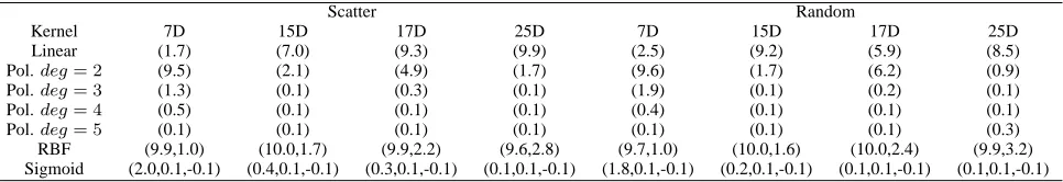
We had four different parameters depending on the kernel function. All kernel functions have one common parameter, box constraint, and whose parameter space was {0.1,0.2, . . . ,10}. RBF has two parameters, σ and box constraint, and they had the same parameter space
{0.1,0.2, . . . ,10}. Sigmoid kernel function has three pa-rameters: box constraint, κ > 0 and δ < 0. For the box constraint andκparameter spaces were the same as before, but nowδ∈ {−10.0,−9.9, . . . ,−0.1}. We tested 100 parameter values in the case of polynomial kernel functions. Furthermore, the RBF and Sigmoid kernel functions were tested with 10000 parameter combinations and for Sigmoid kernel we made an agreement ofκ=−δ
because, otherwise, the number of parameter combina-tions would have increased from 10000 to 1003. The
obtained optimal parameter values can be seen in Table I. HAH-KNN was tested with four different measures. These were Euclidean, cityblock, correlation and cosine. Furthermore, all the tests with HAH-KNN were repeated with oddkvalues from1to51, but only the results with the best kvalues are presented in this paper. The best k
values in each test situation are presented in Tables II-IX.
In feature selection we have used the knowledge from [7]–[10] and one feature set, 17D, was a mixture of 15D and 25D features. Three other feature sets were 7D, 15D and 25D. The data had altogether 25 features and the features can be divided into two categories: simple shape features and grey value features. Features were extracted from the images by using ImageJ [6]. The descriptions of 7D, 15D and 25D feature sets can be found from [8]–[10] and 17D feature set was {Area, Mean, Max, X, Y, XM, YM, Perimeter, BX, BY, Width, Height, Major, Circularity, Feret, Integrated Density, Median}. The definitions of all features can be found from [6] and more details about the preprocessing stage can be found from [27].
A F B D C H E G A vs. F B vs. D C vs. H E vs. G
{AF} vs. {BD} {CH} vs. {EG} {ABDF} vs. {CEGH}
A G B C D F E H
A vs. G B vs. C D vs. F E vs. H {AG} vs. {BC} {DF} vs. {EH}
{ABCG} vs. {DFEH}
Figure 1: Scatter HAH structure on the left and random HAH structure on the right.
Figure 2: Example images of benthic macroinvertebrates. The taxonomic group order of benthic macroinvertebrates is A-H from top left to bottom right.
TABLE I.: The best kernel parameters obtained with the Scatter HAH-SVM and random HAH-SVM
Scatter Random
Kernel 7D 15D 17D 25D 7D 15D 17D 25D
Linear (1.7) (7.0) (9.3) (9.9) (2.5) (9.2) (5.9) (8.5)
Pol.deg= 2 (9.5) (2.1) (4.9) (1.7) (9.6) (1.7) (6.2) (0.9)
Pol.deg= 3 (1.3) (0.1) (0.3) (0.1) (1.9) (0.1) (0.2) (0.1)
Pol.deg= 4 (0.5) (0.1) (0.1) (0.1) (0.4) (0.1) (0.1) (0.1)
Pol.deg= 5 (0.1) (0.1) (0.1) (0.1) (0.1) (0.1) (0.1) (0.3)
RBF (9.9,1.0) (10.0,1.7) (9.9,2.2) (9.6,2.8) (9.7,1.0) (10.0,1.6) (10.0,2.4) (9.9,3.2) Sigmoid (2.0,0.1,-0.1) (0.4,0.1,-0.1) (0.3,0.1,-0.1) (0.1,0.1,-0.1) (1.8,0.1,-0.1) (0.2,0.1,-0.1) (0.1,0.1,-0.1) (0.1,0.1,-0.1)
B. Results
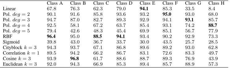
The smallest feature set 7D achieved very good results in [8], [10] when one-vs-one, one-vs-all and DAGSVM were used. The same tendency also continued for the present HAH-SVM case. Tables II and III show the exact results of 7D feature set and different kernel functions. A noticeable observation is that in every result table Sigmoid kernel function obtained the worst results. This may be a consequence from the preprocessing stage where the data was only standardized to have zero mean and unit variance and no transformations such as linear scaling or normalization were made. The results show that randomly formed and with the Scatter method formed HAH-SVMs obtained good results with 7D features. In both cases classes B, D, F, G and H were classified with classification rates above 90% which is an excellent achievement. The rest of the classes were also classified very well since they reached above 88% classification rates. From the kernel functions RBF was the best one in Tables II and III. Also,
the polynomial kernel functions from the cubic to the 5th degree gained good results.
below 90% and in the case of class F cityblock and Euclidean metrics were the only that gained above 90% classification rates. An interesting detail was that class H was recognized only with 66% or lower classification rate. In Table III the HAH-KNN results were similar to results in Table II. Now, class G was the only class in which HAH-KNN obtained the topmost classification rate from all classification rates. The greatest changes in HAH-KNN classification rates between Tables II and III happened in the case of correlation measure. More specifically, classes D, E and G had around 3% change and class H got around 5% change compared to Table II.
Table IV shows the results of 15D feature set. The gen-eral level of the classification rose from the 7D case a bit. Now, RBF kernel function achieved the best classification rate in seven classes from eight possible. Class H was the only that was classified better with other than RBF kernel. Classes D and E were classified with 98.0% and 98.4% classification rates and all the rest of the classes were classified above 90% classification rate. In Table V there is more deviation compared to the previous table. The topmost results were spread over the quadratic, cubic and RBF kernel functions. Overall, the highest classification rates classwise examined did not alternate very much between Scatter and random HAH-SVMs. A surprising aspect is that the linear kernel function did not contrive well in classification although in [8] it gained good results. The reason behind this may be in the structure of HAH-SVM. For instance, in the root node there were training examples from more than two classes to be separated with a single binary SVM, so the input space (or the feature space) is too complicated to be separated with linear kernel function. On the other hand, in one-vs-one method each SVM classifier has only training examples from no more than two classes, and, therefore the space is easier to separate using the linear kernel function.
The results of HAH-KNN in Tables IV and V are interesting because both class division methods produced almost identical results in the cases of all measures tested. Maximum difference between these two division methods was 0.2% in classification rates. A noticeable detail is that in Table IV four classes were identified with the highest classification rates among all methods. Cityblock metric achieved 93.4% classification rate in class A and 97.1% classification rate in class B together with cosine and Euclidean measures. Classes D and G were recognized especially well with cityblock metric since the classifica-tion rates were above 99% and, furthermore, in the case of class D 99.4% classification rate was obtained also by cor-relation and Euclidean measures. Class E was recognized with high classification rate being 96.3% as its highest. In the case of class C cityblock metric gained the highest classification rate 90.2% and it was the only one from the HAH-KNN results which exceeded the limit of 90%. Cityblock and Euclidean metrics were the best alternatives for class F. They obtained above 90% classification rate and from these two metrics the cityblock got the higher one being 92.2%. Class H is an interesting case because
it was clearly the worst classified. Cityblock was again the best option having 79.5% classification rate but when it is compared to RBF or 4th degree polynomial kernel function results, even cityblock clearly remained behind from these two. If this class had been identified with higher classification rate, HAH-KNN would have been comparable with the best HAH-SVM results. A general difference between Tables IV and V is that in the latter only classes D and G were classified better with HAH-KNN than HAH-SVM when in the former classes A, B, D and G were corresponding classes.
In the 17D feature set the level of classification de-creased compared to the previous result tables. Classes C and H were the most difficult to recognize when the HAH-SVM was created by the Scatter method and in the case of a random choice class C was the only one which remained below 90% classification rate. In the Scatter case the topmost classification rates were spread over four kernel functions and in the random HAH-SVM the highest classwise classification rates were distributed within three kernel functions. The cubic kernel function and RBF were the best choices with the 17D feature set. More details about the 17D results can be found from Tables VI and VII.
When considering HAH-KNN results in Tables VI and VII, there are minor changes between the results. The only greater difference was that in the case of class G cityblock metric yielded 93.0% classification rate with Scatter method when in random case the corresponding classification rate was 88.3%. General trend in HAH-KNN results was decreasing compared to the previous tables. In the case of classes A, B, and G above 90% classification rates were achieved by cityblock metric in Table VI. Cosine measure was the best alternative for class B as it was also the best one in 15D results. Now, the classification rate was a bit less than 97%. Cosine mea-sure together with Scatter method obtained around 89% classification rates for D, E and F. Furthermore, cityblock and Euclidean metrics gained above 85% classification rates within these classes. Classes C and H were the poorest ones to be recognized in Tables VI and VII. Both of these classes remained below 70% classification rates with all measures tested. Especially with the correlation and cosine measures the classification rates were below 50% when class H was considered.
TABLE II.: Scatter HAH: Classification rates (%) with kernel functions, measures and 7D feature set.
Class A Class B Class C Class D Class E Class F Class G Class H Linear 41.2 71.8 54.2 84.2 76.9 67.9 0.0 27.6 Pol.deg= 2 76.3 78.1 87.3 83.2 93.5 87.8 78.6 60.4 Pol.deg= 3 87.9 89.2 87.0 92.3 92.3 95.6 87.0 85.7 Pol.deg= 4 88.4 89.4 87.2 93.0 91.2 97.0 92.4 91.8 Pol.deg= 5 85.7 86.5 83.3 92.5 91.4 95.6 92.6 92.2 RBF 89.7 96.1 88.2 98.5 91.4 96.5 93.2 90.2 Sigmoid 53.4 35.9 42.7 46.8 49.1 55.2 41.8 46.2 Cityblockk= 3 87.3 95.5 75.1 95.8 88.1 91.6 97.5 63.6 Correlationk= 1 81.9 90.1 68.0 92.4 67.7 68.1 80.7 50.5 Cosinek= 3 85.8 96.7 77.4 95.8 84.3 86.3 93.9 59.3 Euclideank= 3 85.1 96.2 79.3 95.9 89.1 90.6 96.2 66.0
TABLE III.: Random HAH: Classification rates (%) with kernel functions, measures and 7D feature set.
Class A Class B Class C Class D Class E Class F Class G Class H Linear 93.3 95.2 70.5 34.1 60.4 96.9 14.4 20.8 Pol.deg= 2 87.1 98.3 85.7 80.8 74.0 95.0 87.4 79.9 Pol.deg= 3 91.6 92.4 88.1 87.8 86.6 96.0 94.8 88.6 Pol.deg= 4 88.8 91.3 88.1 91.4 87.5 96.5 93.7 92.4 Pol.deg= 5 84.5 87.3 84.4 91.8 89.0 95.7 95.0 93.2
RBF 91.1 98.7 88.8 98.5 88.2 97.0 96.2 91.3
Sigmoid 78.8 71.7 52.0 54.3 63.7 59.1 61.6 31.9 Cityblockk= 3 87.3 96.5 75.1 95.8 87.3 91.7 97.5 63.6 Correlationk= 3 82.1 90.3 66.2 88.8 70.6 68.3 77.4 55.0 Cosinek= 3 85.8 96.9 77.5 95.8 83.7 86.9 93.9 59.3 Euclideank= 3 85.1 96.7 79.4 95.9 88.7 91.1 96.2 66.0
TABLE IV.: Scatter HAH: Classification rates (%) with kernel functions, measures and 15D feature set.
Class A Class B Class C Class D Class E Class F Class G Class H Linear 73.7 91.2 71.0 58.0 91.6 92.5 68.1 40.3 Pol.deg= 2 90.3 92.8 91.7 93.7 93.8 93.1 84.8 84.7 Pol.deg= 3 90.2 89.8 89.3 91.9 96.9 95.4 90.5 91.5 Pol.deg= 4 87.5 71.8 77.8 76.9 93.3 94.1 87.2 92.4 Pol.deg= 5 76.4 51.5 56.7 51.5 86.8 89.1 76.1 81.9 RBF 92.5 95.9 93.2 98.0 98.4 96.1 94.5 90.7 Sigmoid 48.2 52.5 25.3 47.0 52.2 54.1 28.3 33.5 Cityblockk= 1 93.4 97.1 90.2 99.4 96.3 92.2 99.2 79.5 Correlationk= 1 89.9 97.0 72.4 99.4 91.1 71.6 92.4 62.1 Cosinek= 3 89.8 97.1 78.8 97.3 95.3 94.1 94.9 63.3 Euclideank= 1 91.8 97.1 87.6 99.4 95.3 90.3 97.1 77.6
TABLE V.: Random HAH: Classification rates (%) with kernel functions, measures and 15D feature set.
Class A Class B Class C Class D Class E Class F Class G Class H Linear 81.7 95.4 79.9 85.3 91.8 95.9 49.6 60.5 Pol.deg= 2 93.1 97.1 92.0 89.4 91.7 97.8 92.4 88.9 Pol.deg= 3 94.8 94.1 94.2 88.7 93.2 96.2 96.0 94.5 Pol.deg= 4 88.7 63.4 83.1 63.6 91.5 95.8 92.7 91.6 Pol.deg= 5 76.2 36.9 68.7 39.6 84.6 85.4 86.1 83.7 RBF 92.1 98.4 93.7 98.0 97.1 97.1 98.3 92.1 Sigmoid 21.3 75.0 50.1 47.4 37.4 47.2 45.2 19.1 Cityblockk= 1 93.4 97.1 90.2 99.4 96.3 92.2 99.2 79.5 Correlationk= 1 89.9 97.0 72.4 99.4 91.1 71.6 92.4 62.1 Cosinek= 3 89.8 97.2 78.7 97.3 95.5 94.1 94.9 63.2 Euclideank= 1 91.8 97.1 87.6 99.4 95.3 90.3 97.1 77.6
TABLE VI.: Scatter HAH: Classification rates (%) with kernel functions, measures and 17D feature set.
TABLE VII.: Random HAH: Classification rates (%) with kernel functions, measures and 17D feature set.
Class A Class B Class C Class D Class E Class F Class G Class H Linear 91.4 95.0 74.3 83.3 79.8 94.8 35.1 47.5 Pol.deg= 2 96.9 96.7 87.0 83.6 87.3 96.8 97.3 79.9 Pol.deg= 3 96.1 85.8 89.9 82.1 87.4 96.3 98.0 91.9 Pol.deg= 4 92.3 44.1 70.7 50.7 86.0 95.3 95.1 95.2 Pol.deg= 5 81.8 28.8 59.6 34.5 67.5 83.4 73.7 84.6
RBF 95.6 97.0 88.3 91.6 90.8 94.7 98.1 74.6
Sigmoid 41.2 31.3 25.0 43.8 60.6 54.3 47.0 20.5 Cityblockk= 3 94.1 94.0 67.4 87.9 89.8 89.7 88.3 62.9 Correlationk= 1 89.5 94.2 66.2 86.7 83.1 72.6 83.3 49.7 Cosinek= 3 93.9 96.9 61.4 88.9 88.6 89.8 75.2 43.5 Euclideank= 3 92.0 95.1 67.3 85.3 89.0 86.0 87.7 57.2
TABLE VIII.: Scatter HAH: Classification rates (%) with kernel functions, measures and 25D feature set.
Class A Class B Class C Class D Class E Class F Class G Class H Linear 72.6 91.2 80.4 58.0 91.4 91.6 76.5 35.5 Pol.deg= 2 93.4 92.0 92.2 95.1 96.1 94.9 93.5 84.2 Pol.deg= 3 89.5 80.8 81.5 87.8 91.9 93.1 87.8 88.4 Pol.deg= 4 77.1 60.0 59.3 64.3 79.2 78.6 67.0 79.5 Pol.deg= 5 74.6 51.2 62.4 54.8 69.5 71.5 77.1 77.4 RBF 95.6 95.9 89.8 95.2 94.0 93.0 91.5 81.5 Sigmoid 28.8 49.8 30.6 33.4 32.6 28.5 19.2 30.4 Cityblockk= 3 95.7 95.6 78.6 93.1 92.8 88.4 96.3 64.3 Correlationk= 3 93.4 95.3 64.7 89.0 87.4 78.6 78.0 47.1 Cosinek= 3 96.3 96.7 69.5 90.7 86.7 89.0 80.5 46.0 Euclideank= 9 96.4 94.1 63.1 82.3 91.7 89.0 93.0 58.7
TABLE IX.: Random HAH: Classification rates (%) with kernel functions, measures and 25D feature set.
Class A Class B Class C Class D Class E Class F Class G Class H Linear 83.8 93.4 79.3 86.8 89.1 95.0 58.2 64.8 Pol.deg= 2 96.9 97.1 94.0 87.1 92.0 95.4 95.0 88.8 Pol.deg= 3 91.3 78.4 84.0 71.3 89.3 91.9 94.6 91.7 Pol.deg= 4 79.0 48.7 72.3 49.9 75.6 76.0 88.3 82.7 Pol.deg= 5 73.7 43.3 68.4 44.4 67.0 67.8 84.0 78.7 RBF 95.9 96.4 89.7 92.5 93.1 95.9 97.2 84.6 Sigmoid 42.6 28.5 23.1 33.8 37.9 32.5 36.5 22.4 Cityblockk= 3 95.7 95.6 77.6 93.1 92.2 88.7 96.3 64.3 Correlationk= 3 94.8 95.0 63.6 89.2 87.5 79.6 75.7 46.6 Cosinek= 3 96.3 96.7 69.5 90.9 86.7 90.1 80.5 46.2 Euclideank= 3 94.0 94.3 74.5 90.5 90.6 84.7 92.7 56.0
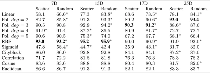
TABLE X.: Mean accuracies from the scatter HAH and random HAH (%) and the results of the statistical tests. Statistical significance between the accuracies obtained by Scatter method and random choice is marked with an asterisk.
7D 15D 17D 25D
Scatter Random Scatter Random Scatter Random Scatter Random Linear 58.1 66.6∗ 77.3 83.8∗ 68.6 78.5∗ 78.1 84.1∗
Pol.deg= 2 82.7 85.8∗ 91.3 93.3∗ 89.2 90.6∗ 93.0 93.4
Pol.deg= 3 90.5 90.8 92.9 94.2∗ 90.3 91.2∗ 88.6∗ 87.6 Pol.deg= 4 91.9∗ 91.4 87.2∗ 86.5 80.9 81.7∗ 72.7 72.7 Pol.deg= 5 90.6 90.5 75.3∗ 74.0 67.2 67.7 68.1∗ 66.4 RBF 93.0 93.2∗ 95.2 95.9∗ 90.0 90.9∗ 91.9 93.0∗
Sigmoid 47.8 58.4∗ 44.7∗ 42.4 35.9 43.1∗ 31.7 32.0 Cityblock 86.0 86.0 92.8 92.8 84.1 84.1 87.2∗ 87.0 Correlation 71.7 72.2 81.8 81.8 76.3 76.3 78.3 78.3 Cosine 83.6 83.6 88.8 88.8 80.4 80.3 81.7 82.0∗
benthic macroinvertebrate images better than 7D feature set although it has over three times more features than in 7D feature set.
HAH-KNN results in Tables VIII and IX are interest-ing. In Table VIII classes A, B and G were classified better by HAH-KNN compared to HAH-SVM results. In the case of class A 96.4% classification rate was achieved by Euclidean metric with k = 3. Moreover, class B was recognized with 96.7% classification rate with cosine measure and class G was identified with 96.3% with cityblock metric. Classes D and E were also identified above 92% classification rates when cityblock metric was used. Class D was classified above 90% classification rate with cosine measure and class E with Euclidean metric. Class F instead gained below 90% classification rates with all measures tested. Again, classes C and H were the hardest classes to be classified with HAH-KNN. Class C achieved below 80% classification rates and especially with other measures than cityblock the results were below 70%. In the case of class H the results were even poorer. All of the tested measures obtained below 70% classi-fication rates and with correlation and cosine measures the results were below 50%. Table IX shows no dramatic changes compared to Table VIII results. All differences were within a 3% interval except with Euclidean metric in the case of classes C, D and F where the differences between Scatter and random divisions were above 4%. Also, only in the case of class D HAH-KNN achieved the highest classification rate when in Table VIII this happened within three classes.
In Table X we see an interesting result. When compar-ing the best accuracies of the Scatter and random columns in each feature set case, we see that the same kernel functions obtained the best performances. Moreover, the difference between the best accuracies using the Scatter method and random choice was below 1%. In every feature set case a random choice produced the better result, but from the practical point of view these results are equally good since their difference was so small. The best feature set choice would be 15D together with RBF kernel function. The 7D and 25D feature sets had quite similar results and the 17D feature set was the poorest one.
In the case of HAH-KNN mean accuracies from ran-dom and Scatter division were nearly identical. The greatest difference between the mean accuracies of Scatter and random divisions was 0.5% and it occurred with 7D feature set when correlation measure was used. With all feature set alternatives cityblock and Euclidean metrics were the best alternatives. With 7D feature set the highest mean accuracies were obtained by Euclidean metric being 86.6% and 86.7%. Furthermore, cityblock metric gained 86.0% mean accuracy with both class division ways. The new feature set, 17D, did not contrive very well since the highest mean accuracy was 84.1% and it was obtained by cityblock metric. However, it needs to be noticed that the mean accuracy of 84.1% was the fourth highest results within the both class division ways when all 17D mean
accuracies are taken into account. The largest feature set, 25D, obtained a bit better mean accuracies com-pared to 17D feature set results. Now, cityblock metric gained 87.2% and 87.0% mean accuracies with Scatter and random divisions and these results are again the fourth highest mean accuracies when HAH-SVM results are taken into account. The best results were obtained with HAH-KNN when 15D feature set was used. The same phenomenom also occurred in HAH-SVM results. Now, with Euclidean metric mean accuracy of 91.3% was gained. Furthermore, with cityblock metric 92.8% mean accuracy was gained which is a very good result. Actually, it is the third highest mean accuracy of 15D results with Scatter division and it is the fourth highest mean accuracy in random division results when 15D feature set was used.
IV. DISCUSSION
In this paper we applied Half-Against-Half multi-class SVMs and a variant Half-Against-Half k-Nearest Neigh-bour (HAH-KNN) method in automated taxa identifica-tion of benthic macroinvertebrates. We formed two Half-Against-Half structures where the one was created by using Scatter method [11] recursively in each node where there was an SVM ork-NN classifier. The other structure was created randomly to have a point of comparison for the structure built by Scatter method. Experimental tests were extensive. We tested four different feature sets and every feature set was tested with seven kernel functions. Furthermore, HAH-KNN was tested with four different measures and with the odd k values from1 to 51. Altogether we made 88 different test arrangements.
In the class division Scatter method worked well al-though it obtained a bit lower accuracies than the random division. Overall, the data was very well classifiable and it may be that even if we made the feature selection and class division in the nodes by using whatever algorithm, we would not get any better results. An important aspect is that there was less than 1% difference between the highest accuracies gained by the random and Scatter methods in each feature set case and despite whether HAH-SVM or HAH-KNN was used. With the HAH-KNN 92.8% mean accuracy was reached with 15D feature set and cityblock metric and this was the best result within all HAH-KNN results. RBF kernel function was the best choice for HAH-SVM and the mean accuracies were 95.2% with Scatter method and 95.9% with random division. Overall, HAH-KNN and HAH-SVM are very promising techniques for benthic macroinvertebrate classification.
it is interesting to apply other classification methods, for instance, linear discriminant analysis, Bayes classifier, Naïve Bayes and Logistic regression with the HAH struc-ture in benthic macroinvertebrate image classification.
ACKNOWLEDGMENT
The author wants to thank Finnish Environment Insti-tute, Jyväskylä, Finland for the data. The author is also thankful to the Tampere Graduate Program in Informa-tion Science and Engineering and Maj and Tor Nessling Foundation for the support. The author also wants to thank Markku Siermala, Ph.D., for the Scatter method and Jorma Laurikkala, Ph.D., for statistical tests.
REFERENCES
[1] K.J. Cios, W. Pedrycz, R.W. Swiniarski and L.A. Kurgan,
Data Mining: A Knowledge Discovery Approach,
Springer-Verlag, 2007.
[2] C. Cortes and V. Vapnik, “Support-vector networks,”
Ma-chine Learning, Vol. 20, No.3, pp. 273–297, 1995.
[3] R.O. Duda, P.E. Hart and D.G. Stork, Pattern
Classifica-tion, John Wiley & Sons, 2nd ed., 2001.
[4] K.J. Gaston and M.A. O’Neill, “Automated species identi-fication: why not?,” Philophical Transactions of the Royal
Society B, pp. 359, 655–667, 2004.
[5] T. Howley and M.G. Madden,“The genetic evolution of kernels for support vector machine classifiers,”
Proceed-ings of AICS-2004 15th Irish Conference on Artificial Intelligence & Cognition Science, 2004.
[6] ImageJ:public domain Java-based image processing pro-gram. Available: http://rsbweb.nih.gov/ij/
[7] H. Joutsijoki, “Half-Against-Half support vector machines in classification of benthic macroinvertebrate images,”
Pro-ceedings of 2012 International Conference on Computer and Information Science (ICCIS 2012), IEEE, Vol. 1, pp.
414–419, 2012.
[8] H. Joutsijoki and M. Juhola, “Comparing the one-vs-one and one-vs-all methods in benthic macroinvertebrate im-age classification,” Lecture Notes in Artificial Intelligence, 6871, Springer-Verlag, pp. 399–413, 2011.
[9] H. Joutsijoki and M. Juhola, “Kernel selection in multi-class support vector machines and its consequence to the number of ties in majority voting method,” Artificial
Intelligence Review, Vol. 40, No. 3, pp. 213–230, 2013.
[10] H. Joutsijoki and M. Juhola, “Automated benthic macroin-vertebrate identification with decision acyclic graph sup-port vector machines,” Proceedings of the IASTED 2nd
International Conference on Computational Bioscience,
pp. 323–328, 2011.
[11] M. Juhola and M. Siermala, “A scatter method for data and variable importance evaluation,” Vol. 19, No. 2, Integrated
Computer-Aided Engineering, pp. 137–149, 2012.
[12] S. Kiranyaz, M. Gabbouj, J. Pulkkinen, T. Ince and K. Meissner, “Network of evolutionary binary classifiers for classification and retrieval in macroinvertebrate databases,”
Proceedings of 2010 IEEE 17th International Conference in Image Processing, pp. 2257–2260, 2010.
[13] S. Kiranyaz, M. Gabbouj, J. Pulkkinen, T. Ince and K. Meissner, “Classification and retrieval on macroinverte-brate image databases using evolutionary RBF neural networks,” Proceedings of the International Workshop on
Advanced Image Technology, 2010.
[14] S. Kiranyaz, T. Ince, J. Pulkkinen, M. Gabbouj, J. Ärje, S. Kärkkäinen, V. Tirronen, M. Juhola, T. Turpeinen, K. Meissner, “Classification and retrieval on macroin-vertebrate image databases,” Computers in Biology and
Medicine, Vol. 41, No.7, pp. 463–472, 2011.
[15] N. Larios, J. Lin, M. Zhang, D. Lytle, A. Moldenke, L. Shapiro and T. Dietterich, “Stacked spatial-pyramid kernel: An object-class recognition method to combine scores from random trees,” 2011 IEEE Workshop on Applications
of Computer Vision (WACV), pp. 329–335, 2011.
[16] N. Larios, B. Soran, L. G. Shapiro, G. Martinez-Muñoz, J. Lin and T. G. Dietterich, “Haar random forest features and SVM spatial matching kernel for stonefly species identifi-cation,” Proceedings of 20th International Conference on
Pattern Recognition (ICPR), pp. 2624–2627, 2010.
[17] H. Lei and V. Govindaraju, “Half-Against-Half multi-class support vector machines,” Lecture Notes in Computer
Science, 3541, Springer-Verlag, pp. 156–164, 2005.
[18] D.A. Lytle, G. Martinez-Muñoz, W. Zhang, N. Larios, L. Shapiro, R. Paasch, A. Moldenke, E.N. Mortensen, S. Todorovic and T.G. Dietterich, “Automated processing and identification of benthic invertebrate samples,” Journal of
North American Benthological Society, Vol. 29, No.3, pp.
867–874, 2010.
[19] G. Martinez-Muñoz, W. Zhang, N. Payet, S. Todorovic, N. Larios, A. Yamamuro, D. Lytle, A. Moldenke, E. Mortensen, R. Paasch, L. Shapiro, and T. Dietterich, “Dictionary-free categorization of very similar objects via stacked evidence trees,” Proceedings of IEEE Conference
on Computer Vision and Pattern Recognition (CVPR), pp.
549–556, 2009.
[20] M.A. Pett, Nonparametric Statistics for Healt Care
Re-search: Statistics for Small Samples and Unusual Distri-butions, SAGE Publications, 1997.
[21] J. Saarikoski, J. Laurikkala, K. Järvelin and M. Juhola, “A study of self-organising maps in information retrieval,”
Journal of Documentation, Vol. 54, No. 2, pp. 304–322,
2009.
[22] J. Saarikoski, J. Laurikkala, K. Järvelin and M. Juhola, “Self-Organising maps in document classification: A com-parison with six machine learning methods,” Lecture Notes
in Computer Science, 6593, pp. 260–269, 2011.
[23] M.J. Sarpola, R.K. Paasch, E.N. Mortensen, T.G. Di-etterich, D.A. Lytle, A.R. Moldenke and L.G. Shapiro, “An aquatic insect imaging system to automate insect classification,” Transactions of the ASABE, Vol. 51, No.6, pp. 2217–2225, 2008.
[24] S. Siegel and N.J. Jr. Castellan, Nonparametric Statistics
for the Behavioral Sciences, McGraw-Hill, 1988.
[25] J.A.K. Suykens and J. Vandewalle, “Least squares support vector machine classifiers,” Neural Processing Letters, Vol. 9, pp. 293–300, 1999.
[26] V. Tirronen, A. Caponio, T. Haanpää and K. Meissner, “Multiple order gradient feature for macro-invertebrate identification using support vector machines,” Lecture
Notes in Computer Science, 5495, pp. 489–497, 2009.
[27] J. Ärje, S. Kärkkäinen, K. Meissner and T. Turpeinen, “Statistical classification and proportion estimation - an application to a macroinvertebrate image database,”
Pro-ceedings of 2010 IEEE International Workshop on Ma-chine Learning for Signal Processing (MLSP 2010), pp.
373–378, 2010.
[28] V.N. Vapnik, The Nature of Statistical Learning Theory, 2nd edition, Springer, 2000.
Henry Joutsijoki received his M.Sc. and Phil.Lic. degrees