Neural Network Adaptive Control for a Class of Matched SISO Nonlinear Uncertain Systems with Zero Dynamics

Neural Network Adaptive Control for a Class of

Matched SISO Nonlinear Uncertain Systems with

Zero Dynamics

Hui Hu

Dept of Electrical and Information Engineering, Hunan Institute of Engineering, Hunan Xiangtan, China Email: [email protected]

Peng Guo

Dept of Computer Science, Hunan Institute of Engineering, Hunan Xiangtan, China Email:[email protected]

Abstract

—

The paper presents a direct adaptive tracking control scheme for a class of matched SISO affine nonlinear uncertain systems with zero dynamic using neural network. Through neural network approximation, neural network is used as the emulator of the unknown ideal controller. A quadratic cost function of the error between the unknown ideal controller and the used neural network controller is minimized using a gradient descent method to adjust parameters in neural network. The convergence of parameters and the uniformly ultimately boundedness of tracking error and all states of the closed-loop system are guaranteed based on Lyapunov stability theorem. The effectiveness of the proposed controller is illustrated through the simulation results.

Index Terms

—

tracking control, matched uncertain nonlinear, gradient descent method, neural network, zero dynamic

I. INTRODUCTION

There are some inevitable uncertainties in actual system which will cause instability and difficulties in dealing with system. Therefore, the study of uncertain nonlinear system is of vital importance. Control of uncertain nonlinear dynamic systems is still a challenging problem though it attracted many researchers in control community during the past few decades led to development of fruitful methods based on adaptive control concepts. Alternatively, in recent years, adaptive neural network [3, 7, 8, 9, 10, 12, 19, 20, 22, 25] and fuzzy logic control [1, 2, 5, 6, 13, 14, 15, 16, 17, 18, 21, 23] become an active research area. These methodologies become especially more helpful if control of highly uncertain, nonlinear and complex systems is the design issue. The main philosophy that is exploited heavily in system theory applications is the universal function approximation property of neural networks or fuzzy logic. Benefits of using neural networks or fuzzy logic for control applications include its ability to effectively control nonlinear plants while adapting to unmodeled dynamics. In general, a two-step procedure is taken. First, based on implicit function theorem an ideal controller developed to

stabilize the underlying system and make the tracking approach a neighborhood of zero. Then, a neural network or fuzzy logic to approximate this ideal controller is designed. Based on the Lyapunov stability analysis, an adaptation law is devised to update the adjustable parameters. However a bounding controller may also be added for more performance robustness. In the above most methods the parameter adaptation laws are designed based on a Lyapunov approach, where an error signal between the desired output and the actual output is used to update the adjustable parameters and the control laws are composed of three control terms: a linear control term, an adaptive neural network control term and a robustifying control term used to compensate for disturbances and approximation errors. On the other hand, almost all of the above works don’t considered the zero dynamics, though it plays an important role in nonlinear system control. Considering that zero dynamics exist in many practical systems, including isothermal continuous stirred tank reactors, aircraft trajectory tracking control systems and others, it is necessary to investigate their influence on nonlinear system. In the paper, according to [5], we introduce a direct adaptive neural network control approach for a class of matched SISO affine nonlinear uncertain systems with zero dynamics. The basic idea is to use neural network to adaptively construct an unknown ideal controller and the parameter adaptive laws is designed ,based on the gradient descent method, to directly minimizing the error between the unknown ideal controller and the neural network controller And no robustifying control term is used in controller. This paper proves the availability of the method in both theory and simulation experiment.

II. PROBLEM FORMULATION

Consider the following matched SISO affine nonlinear uncertain system:

(

)

( ) ( ) ( ) ( )

( )

x f x f x g x g x u

y h x

= + Δ + + Δ

⎧ ⎨

=

⎩ (1)

Where_x∈Rnand _{u y}, _∈R are system state, system input

and output respectively. n

x R

Ω ⊂ , Ω ⊂u R are two

compact sets. f x( )and g x( )are smooth vector fields.

( )

f x

Δ and Δg x( )are bounded uncertain terms.h x( )∈ R is smooth scalar function.

Assumption 1: Nominal system(1)possesses a strong

relative degree r<n .

x

f x

_{( )}

( )

g x u

( )

y

h x

=

+

⎧

⎨

=

⎩

(2)

Assumption 2: Uncertainties meet the match conditions.

1

2 ( ) ( ) ( ) ( )

f x g x x

g x g x x

δ δ

Δ = ( )

Δ = ( )

(3)

According to differential geometry theory of nonlinear system, we know that there is a nonlinear transformation

(

_T, _T

)

T

x ξ η

Τ( ) = , which turns system(1)to

[

]

{

}

1

1 2

1

1

( , ) ( , ) ( ) 1 ( ) ( , )

i i

r

d

i r

dt d

x x u

dt q y

ξ _ξ

ξ _{α ξ η β ξ η δ δ}

η ξ η

ξ

+

= = 1, , −

= + + +

=

=

⎧ ⎪ ⎪ ⎪ ⎨ ⎪ ⎪ ⎪ ⎩

(4)

where i 1 _{( )}

i L h xf

ξ ₌ − _{， ( , )} r _{( )}

f

L h x

α ξ η = and

1

( , ) r ( ) 0

g f

L L h x

β ξ η ₌ − _{≠ . For all}

( )

_,

x

x u ∈ Ω × R

t

he functionβ ξ η( , ) is nonzero and bounded. This implies that β ξ η( , ) is strictly either positive or negative. Without loss of generality, it is assumed that it exists a positive constant

c

such that β ξ η( , )≥ >c 0 for all

( )

x u, ∈ Ω × x R .

Assumption 3: For all_{x∈ R}n , we have

1+δ2( )x ≥ϑ( ) 0x > (5)

Assumption 4: Zero dynamics d q(0, )

dt

η _{= η is}

exponentially stable, and the function ( , )qξ η is Lipschitz in ξ

.

By Lyapunov converse theorem[11]_{, there is a} Lyapunov function V0( )η which satisfies

2 2

1 V0( ) 2

σ η ≤ η σ η≤ (6) 2

0

3

( ) _{(0, )}

V q

η _{η σ η}

η

∂ _{≤ −}

∂ (7)

0

4 ( ) V η

σ η η

∂ _≤

∂ (8)

Whereσi,i=1,2,3,4 are positive constant.

( , ) (0, )

qξ η −q η ≤L_ξ ξ (9) Where L_ξ is Lipschitz constant.

Define the reference vector ( 1)

( r )T r

d d d d

y = y y y − ∈R

The reference signal

y

d and its time derivative are

assumed to be smooth and bounded. We also define the tracking error as

d

e= y −y

and corresponding error vector as ( 1)

( , , r )T r

e= e e e − ∈R

Then the error equation in the new coordinate is as follows:

[

]

{

}

( )

0 dr ( , ) ( , ) 1( ) 1 2( )

e=A e+b y⎡_⎣ −α ξ η β ξ η δ− x + +δ x u ⎤_⎦

(10)

Where 0

0 1 0 0

0 0 1 0

0 0 0 1

0 0 0 0 0 _{r r}

A

×

⎡ ⎤

⎢ ⎥

⎢ ⎥

⎢ ⎥

=

⎢ ⎥

⎢ ⎥

⎢ ⎥

⎣ ⎦

,

1

0 0 0

1 _r

b

×

⎡ ⎤ ⎢ ⎥ ⎢ ⎥ ⎢ ⎥

=

⎢ ⎥ ⎢ ⎥ ⎢ ⎥ ⎣ ⎦

.

Obviously, if

(

A b0,

)

can be controllable, then there will exist a constant matrix

[

0, ,1 1

]

T r

K= k k k₋ which makes eigenvalues of matrix Ac=A0−bKT all have negative real part. Thus, for any given positive definite symmetric matrix

Q

, there exists a unique positive definite

symmetric solution

P

to the following Lyapunov

algebraic equation: T

c c

A P+PA = −Q (11) The control objective is to design an adaptive neural network controller for a class of matched SISO affine nonlinear systems (1) such that the system output follows a desired trajectory while all signals in the closed-loop system remain bounded.

Assumption 5: Desired output

y

d and its r-order time

derivative are assumed to be smooth and bounded. Then there exists a positive constant bdwhich makes

(1) ( )

( r )T

d d d d

y y y ≤b

(12)

III. DESIGN OF CONTROLLER Define a signal

( )

= r T tanh T

d

b Pe

y K e

ν + +λ ⎛⎜ ⎞⎟

Ξ

where tanh( )• is the hyperbolic tangent function, ,Ξ λare the positive design parameters tanh( ) ( 1,1)• ∈ − , when error e→ ∞+ , the value of tanh +

T

b Pe

⎛ ⎞

→ ∞

⎜ ⎟

Ξ

⎝ ⎠ . And

when error e→ ∞- _{,the value of} tanh

-T

b Pe

⎛ ⎞

→ ∞

⎜ _Ξ ⎟

⎝ ⎠ .

When e→0 , tanh 0

T

b Pe

⎛ ⎞

→

⎜ ⎟

Ξ

⎝ ⎠ .The term

tanh b PeT

λ ⎛⎜ _Ξ ⎞⎟

⎝ ⎠

is a

smooth approximation of the

discontinuous term

(

T

)

sign b Pe

λ usually used in robust control. So, λ

is

selected larger than the magnitude of the uncertainty and it will affect the convergence rate of the tracking error, and Ξ is chosen very small to best approximate the sign function and it will affect the size of the residual set to which the tracking error will converge. The sign function is not used here to avoid problems associated with it as chattering and solutions existence.

By adding and subtracting ν in (10), we obtain

(

)

(

)

{

}

0

1 2

tanh

( , ) ( ) 1 ( )

T

T b Pe

e A bK e b

b x x u

λ

α ξ η β δ δ ν

⎛ ⎞

= − − ⎜ _Ξ ⎟−

⎝ ⎠

⎡ ⎤

+ _⎣ + + + − _⎦

(13)

if

δ

₁( ), ( )x

δ

₂ x are known, there exists some ideal

controller *_{( )}

u z satisfying the following equality :

[

]

(

)

1

(

)

*

2 1

( ) ( , ) 1 ( ) ( , ) ( , ) ( )

u z = β ξ η +δ x − v−α ξ η β ξ η δ− x

(14) The closed-loop error dynamic is reduced to (15)

(

0

)

tanh

T

T b Pe

e= A −bK e−bλ ⎛_⎜ ⎞_⎟ Ξ

⎝ ⎠ (15)

Considering the following Lyapunov function: T

V =e Pe (16) According to (11) and (15), we have

_{V = −e Qe}T ₋2λ_{b Pe}T tanh⎛b PeT ⎞

⎜ ⎟

Ξ

⎝ ⎠ (17)

Since the term _{b Pe}T tanh⎛b PeT ⎞

⎜ _Ξ ⎟

⎝ ⎠ is always

positive,we conclude that V ≤0 ,and only when

0

e

=

,V =0 which means lim | | 0 t→∞ e = .

However, in ideal controller (14) δ1( ), ( )x δ2 x are unknown ,so *_{( )}

u z is not available. In what follows, a neural network will be used to construct the unknown ideal controller.

In control engineering, radial basis function (RBF) NNs are usually used as a tool for modeling nonlinear functions because of their good capabilities in function approximation. In this paper, the following RBF NN

( ) T( )

u z =φ zθis used to approximate the ideal controller *_{( )}

u z , where _z=⎡ξ ηT, ,T _v⎤T

⎣ ⎦ , θ =( , ,θ1 θM)T is the

adjustable parameter, and φ( ) ( ( ), , ( ))z = φ1 z φM z Tis the

basic function vector. It has been proven that network can approximate any smooth function over a compact set

q

Z R

Ω ⊂ to arbitrarily any accuracy as

*_{( )} T_{( )} * _{( )}

u z =φ zθ δ+ z (18) with bounded function approximation error δ( )z satisfying δ( )z ≤δ .Where θ* is an ideal parameter vector which minimizes the function δ( )z .In this paper ,we assume that the used neural network does not violate the universal approximation property on the compact set ΩZ,which is assumed large enough so that

the variable zremains inside it under closed-loop control. RBFNN represents a class of linearly parameterized approximators and can be replaced by any other linearly parameterized approximators such as spline functions[24] or fuzzy systems[23]. Moreover, nonlinearly parameterized approximators, such as multilayer neural network(MNN), can be linearized as linearly parameterized approximators, with the higher order terms of Taylor series expansions being taken as part of the modeling error, as shown in [19],[20].

Let us define the error between the controllers u z( )and

*_{( )} u z as

*_{( ) ( )} T_{( ) ( )} u

e =u z −u z =φ zθ δ+ z (19) Where _{θ θ θ=} *_{− is the parameter estimation error vector.} By substituting *_{( )}

u z into the equation (13) and considering (19), we get

[

]

[

]

[

]

[

]

[

]

(

)

1

*

2 2

* 2

* 2

c

c

tanh ( , ) ( , ) ( )

- ( , ) 1 ( ) ( , ) 1 ( ) ( ) - ( , ) 1 ( ) ( )

= tanh ( , ) 1 ( ) ( ) ( )

T

T

b Pe

e A e b b x v

b x u x u z

x u z

b Pe

A e b b x u z u z

λ α ξ η β ξ η δ

β ξ η δ β ξ η δ

β ξ η δ

λ β ξ η δ

⎛ ⎞

= − ⎜ ⎟− + − −

Ξ

⎝ ⎠

⎡ _{+ + + −}

⎣

⎤

+ _⎦

⎛ ⎞

− ⎜ ⎟− + −

Ξ

⎝ ⎠

(20) Considering Ac=A0−bKT, then (20) can be rewritten as

( )

[

]

2

tanh T ( , ) 1 ( )

r T

u

b Pe

e +K e+λ ⎛⎜ ⎞⎟=β ξ η +δ x e

Ξ

⎝ ⎠ (21)

We notice here that *_{( )}

u z is an unknown quantity , so the signal eudefined in (19) is not available. Eq.(21) will be

used to overcome the difficulty. Indeed ,from(21), we see that even if the signaleuis not available for measurement,

will be exploited in the design of the parameters adaptive law.

Now, consider a quadratic cost function defined as

[

]

₂

[

]

(

_*

)

2

2 2

1 _{1 ( )} 1 _{1 ( ) ( ) ( )}

2 2

T u

J_θ = +δ x e = +δ x u z −φ zθ (22)

By applying the gradient descent method, we obtain as an adaptive law for the parameters θ

[

2

]

( ) 1 ( ) ( ) u

J x z e

θ

θ = − ∇γ θ =γ +δ φ (23)

Since

e

uand

δ

2

( )

x

are not available, the adaptive law (23) can not be implemented. In order to render (23) computable ,from Eq.(21), we select the design parameter ( , ) θ γ γ β ξ η= , where γ_θ is a positive constant. At the same time ,to improve the robustness of adaptive law in the presence of the approximation error ,we modify it by introducing a σ -modification term as follows:

[

]

(

2

)

( ) ( ) ( , ) 1+ ( ) = ( ) tanh u T r T z x e b Pe z e K e θ θ θ θ γ φ β ξ η δ σθ γ φ λ γ σθ = − ⎧ ⎛ ⎞⎫ ⎪ _{+ +} ⎪₋ ⎨ ⎜ ⎟⎬ Ξ ⎪ ⎝ ⎠⎪ ⎩ ⎭ (24) where σ is a small positive constant Because the aim of the σ -modification adaptive law is to avoid parameter drift, it does not need to be active when the estimated parameters are within some acceptable bound. The proposed adaptive controller is only composed of a neural network part without additional control terms and the system stability relies entirely on the neural network. The term λtanh⎛⎜b PeT ⎞⎟ Ξ ⎝ ⎠ in the parameter adaptive law (24) plays, in some way, the role of a robustifying control term. Thus the robustness of the controller can be improved by selecting a large positive value for the design parameterλ and a small positive value for the parameterΞ. IV. CONVERGENCE AND STABILITY ANALYSIS OF CONTROL SYSTEM Firstly, let us consider the convergence of neural network parameters. Considering the following positive function: = 1

2 T V_θ θ θ θ γ (25)

Using (19) and (24), the time derivative of (25) can be written as

(

)

(

)

(

)

(

)

(

)

2 2 2 2 2 - ( ) ( , ) 1 ( ) - ( ) ( , ) 1 ( )

( , ) 1 ( ) ( , ) 1 ( ) ( ) T u T T u T u u V z x e z x e x e x z e θ θ φ β ξ η δ σθ φ θβ ξ η δ σθ θ β ξ η δ β ξ η δ δ σθ θ = + = + + = − + + + + (26) Using the inequalities 2 2 2 2 _* 2 2 2 2 2 2 T σ σ σ σθ θ θ θ θ θ σ _θ σ _θ = − − + + ≤ − + (27)

(

)

2 2 2 2 2 2 1 1 1 ( ) ( ) ( ) 2 2 2 1 1 ( ) 2 2 u u u u u e z e e z e z e z δ δ δ δ − + = − + − − ≤ − + (28)

Considering (27) and (28), Eq.(26) can be bounded as

(

)

2

(

)

2 2 2 2 _* 2 1 _{( , ) 1 ( )} 1 _{( , ) 1 ( ) ( )} 2 2 2 2 u V_θ β ξ η δ x e β ξ η δ x δ z σ _θ σ _θ ≤ − + + + − − + (29)

Since the parameters _θ* _{are constants, and the functions} ( )z δ and β ξ η δ( , ), ( )2 x are assumed bounded in this paper, so we can define a positive constant bound ψ as

(

)

_{2 *} 2 2 1 sup ( , ) 1 ( ) ( ) 2 2 t x z σ ψ = ⎛⎜ β ξ η +δ δ ⎞⎟+ θ ⎝ ⎠ (30)

Then

(

)

2 2 1 _{1 ( , ) 1 ( )} 2 2 u V V x e V θ θ θ ρ ψ β ξ η δ ρ ψ ≤ − + − + ≤ − + (31)

where ρ σγ= θ .Eq.(31) implies that for V_θ >ψ_ρ ,V_θ<0 and , therefore, θ is bounded. By integrating (31), we can establish that: 2 2 (0) t 2 e ρ _θψ θ θ γ ρ − ≤ + (32)

From (32) we have ₍₀₎ 0.5 t ₂ e ρ _θ θ _≤ θ − ₊ γ ψ ρ ₍₃₃₎

Using (33) and the fact that δ( )z and β ξ η δ( , ), ( )2 x are bounded, we can write

(

)

(

)

(

)

(

)

(

)

(

)

2 2 2 2 2 ( , ) 1 ( ) ( ) ( ) ( , ) 1 ( ) ( ) +

+ ( , ) 1 ( ) ( )

( , ) 1 ( ) ( ) +

+ ( , ) 1 ( ) ( )

T T T x z z x z x z x z x z β ξ η δ φ θ δ β ξ η δ φ θ β ξ η δ δ β ξ η δ φ θ β ξ η δ δ + + ≤ + + ≤ + +

(

)

(

)

(

)

0.5 2 2 2 0.5 0 1 ( , ) 1 ( ) ( ) (0) ( , ) 1 ( ) ( ) 2 + + ( , ) 1 ( ) ( )

T t

T

t

x z e

x z

x z

e

ρ

θ

ρ

β ξ η δ φ θ

β ξ η δ φ γ ψ ρ

β ξ η δ δ

ψ ψ

−

−

≤ + +

+ +

+

≤ +

where ψ ψ0, 1 are some finite positive constants.

Lemma 2[11]: The following inequality holds for all

0

Ξ > and ς∈R withK_c=0.2785.

0 tanh Kc

ς

ς ς ⎛ ⎞

≤ − ⋅ ⎜ ⎟_Ξ ≤ Ξ

⎝ ⎠ (35)

Theorem 1: Consider the system (1).Suppose that

Assumption1-5 are satisfied, then the neural network controller and adaptation law given by (24) guarantees the convergence of the neural network parameters and to be uniformly ultimately bounded of all the signal in the closed-loop system.

Proof: Consider the Lyapunov function candidate: V e( , )η =e PeT +μ ηV0( ) (36) Differentiating (36) with respect to time and using (11),(20),(34),(35),and lemma 1,we have

0 tanh Kc

ς

ς ς ⎛ ⎞

≤ − ⋅ _{⎜ ⎟}≤ Ξ

Ξ

⎝ ⎠

with Kc=0.2785,we obtain

(

)

(

)

(

)

(

)

* 2 0 2 0

( ) 2 tanh

+2 ( , ) 1 ( ) ( ) ( )

2 tanh

+2 ( , ) 1 ( ) ( ) ( ) ( )

2 tanh

T

T T T

c c T T T T T T T T T b Pe V e e A P PA e b Pe

b Pe x u u V

b Pe e Qe b Pe

b Pe x z z V

b P e Qe b Pe

λ β ξ η δ μ η λ β ξ η δ φ θ δ μ η λ ⎛ ⎞ = + − ⎜ ⎟+ Ξ ⎝ ⎠ + − + ⎛ ⎞ =− − ⎜ ⎟+ Ξ ⎝ ⎠ + + +

≤− −

(

0.5

)

0 1 0

0.5

0 1 0

2 ( )

2 2 ( )

T t

T T t

c

e

b Pe e V

e Qe b Pe e K V

ρ ρ ψ ψ μ η ψ ψ μ η − − ⎛ ⎞ + + ⎜ ⎟ Ξ ⎝ ⎠ ≤− + + Ξ+ (37) Considering assumption 4, we have

[

]

0.5

0 1

0

( , ) 2 2

( )

(0, ) ( , ) (0, )

T T t

c

V e e Qe b Pe e K

V

q q q

ρ η ψ ψ η μ η ξ η η η − ≤ − + + Ξ + ∂ + + − ∂ 2

3 4 2 1

T

c

e Qe μσ η μσ L_ξ ξ η ψ K

≤ − − + + Ξ

(38)

Considering assumption 5 and

(1) ( 1)

( r )T

d d d d

e y y y e b

ξ _{≤ +} − _{≤ +}

Then

2 2

min 3 4

4 1

( , ) - ( )

d 2 c

V e Q e L e

L b K

ξ ξ η λ μσ η μσ η μσ η ψ ≤ − + + + + Ξ (39) Using the inequality

2 2

4 4 1 4

1

1 1

2 2

L e_ξ L_ξ L e_ξ

μσ η μσ ε η μσ

ε

≤ + (40)

(

)

2 2

4 4 2 2

2 1 4

d d

L b_ξ L_ξ b

μσ η μσ ε η

ε

≤ +

(41)

Then (39) satisfies

(

)

(

)

2 2 2

min 3 4 1

2

2 2

4 4 2 2 1

1 2

2

min 4 2 1

1 2

2 2

3 4 1 4 2

1 ( , ) - ( ) 2 1 1 2 2 4 1 1

- ( ) 2

2 4 1 2 d c c d

V e Q e L

L e L b K

Q L e K

L L b

ξ ξ ξ ξ ξ ξ η λ μσ η μσ ε η μσ μσ ε η ψ ε ε λ _ε μσ ψ ε μ σ σ ε μ σ ε η ≤ − + + + + + Ξ ⎛ ⎞ ≤ ⎜ − ⎟ + + Ξ − ⎝ ⎠ ⎡ ⎤ − _⎢ − − _⎥ ⎣ ⎦ …

(42) Where ε ε1, 2 are suitable positive constants. Adjusting

1, 2

ε ε to make 3 1 4 1

(

4 2

)

2 0

2 Lξ Lξ bd

σ − σ ε μ σ ε− > .

Selecting

(

)

3 4 1

2 4 2 1 1 2 2 d L L b ξ ξ σ σ ε μ σ ε ⎛ ⎞ − ⎜ ⎟ ⎝ ⎠

= , then

(

)

2

3 4 1

2 2

min 4 2

1 _{4 2}

1

1 1 2

( , ) ( ) 0.5

2 4

d

L

V e Q L e

L b ξ ξ ξ σ σ ε η λ _ε μσ η ε σ ε ⎛ ₋ ⎞ ⎜ ⎟ ⎛ ⎞ _{⎝ ⎠} ≤ −⎜ − − ⎟ − + ⎝ ⎠ (43)

Where 2 2

0 1

2 2

1 _{2 2}

4

T t

c

b P eρ K

ε_{= ε +} ψ − ₊ ψ _{Ξ. Selecting Q}

to make min 4

1 1

( ) 0.5 0

2

Q L_ξ

λ − − _ε μσ > . From the above equation, we can know that tracking error and internal statesη are all uniformly ultimately bounded. Besides,

since ₍ (1) ( 1)r ₎T

d d d d

e y y y e b

ξ _{≤ +} − _{≤ +}

_,

then the state ξ is uniformly ultimately bounded too. This completes the proof.

VI. SIMULATION STUDY

In this section, to illustrate the validity of the proposed adaptive neural network controller, the following SISO affine nonlinear uncertain system with zero dynamics is simulated. The affine nonlinear system is described by the following differential equation:

2

1 1 1 2

2

2

0

4 2 _{( ) ( )}

1 0

x x x x

f x g x u

x y x ⎛ ⎞ ⎡_{− +} ⎤ ⎡ ⎤ ⎡ ⎤ =⎢ ⎥+ Δ +⎜ + Δ ⎟ ⎢ ⎥ ⎢ ⎥ ⎣ ⎦ ⎣ ⎦ ⎣ ⎦ ⎝ ⎠ = (44) where 1 0 ( ) 0.1sin f x x ⎡ ⎤ Δ =⎢ ⎥

⎣ ⎦ , 2

0 ( ) 0.1sin g x x ⎡ ⎤ Δ =⎢ ⎥

⎣ ⎦ .The

the desired trajectory yd =sint+2cos(0.5 )t .The relative

degree r=1

.

Selecting nonlinear

transformation ( ) ,

[

2, 1

]

T T

T T

T x =⎡_⎣ξ η ⎤_⎦ = x x

,

then the zero dynamic x1= −4x1 which is exponential stable. We knowδ1( ) 0.1sinx = x1and δ2( ) 0.1sinx = x2

satisfy the

matched condition.

The system initial conditions are

[

]

(0) 2 1T

x = .The design parameters used in this

simulation are selected as follows Q=diag[10,10] , 15 5

5 5 P=⎡_⎢ ⎤_⎥

⎣ ⎦ ,

[ ]

1,2 T

K= ,

0.03

Ξ = ,γ =θ 6,σ =0.08.The simulation result is shown in Fig1,2,3,4.

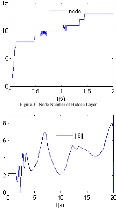
The simulation result for the output is shown in Fig.1 ,and the control input signal is shown in Fig.2. the node changes are shown in Fig.3. Fig.4 shows the evolution of the Euclidian norm of the parameter estimates It can be seen that the actual trajectories converge rapidly to the desired ones. The computer simulation results show that the adaptive neural network controller can perform successful control and achieve desired performance.

Figure 1. Plots of output tracking of system

Fig.2 Plots of Control input

Figure 3 Node Number of Hidden Layer

Fig 4.Norm of the weight vector θ

V. CONCLUSIONS

In this paper, a new adaptive neural network control scheme is presented for a class of matched SISO affine nonlinear uncertain systems with zero dynamics. The error between ideal controller and neural network controller is used to update the adjustable parameters by the gradient descent algorithm. The overall adaptive scheme guarantees that all signals involved are uniformly ultimately bounded and the output of the closed-loop system tracks the desired output trajectory. Simulation results show the controller can achieve a satisfactory performance.

ACKNOWLEDGMENT

REFERENCES

[1] Liu G R,Wan B W. “Indirect adaptive fuzy robust control for a class of nonlinear MIMO systems”.Control and Decision,vol.17,pp.676-680,2002.

[2] Tong S C,Qu L J. “Fuzzy adaptive output feedback control for a class of MIMO nonlinear systems”.Control and Decision,vol.27,781-793,2005.

[3] Hu H, Liu G R,Tang H Z,Guo Peng. “Robust output tracking control for mismatched uncertainties nonlinear systems”, Natural Science Journal of Xiangtan University,vol.32,pp.108-111,2010.

[4] Chen W,Wang Y N,Huang H X. “L2 robust control of induction motor based on backstepping”,Natural Science Journal of Xiangtan University,vol.32,pp.106-111,2010. [5] Salim L, Thierry M G. “Adaptive fuzzy control of a class of

SISO nonaffine nonlinear systems”.Fuzzy Sets and Systems,vol.158,pp.1126-1137,2007.

[6] Huang H X,Nuan T. “Application of adaptive fuzzy sliding mode control based on GA in positioning servo system of the permanent magnetic linear motors”, Natural Science Journal of Xiangtan University,vol.32,pp.94-98,2010. [7] Chang Y C,Yen H M. “Adaptive output feedback tracking

control for a class of uncertain nonlinear systems using neural networks”.IEEE Trans on systems,man,and cybernetics-part B:cybernetics,vol. 36,pp.1311-1316,2005. [8] Sunan N H,Tan K K,T.H.Lee. “Further results on adaptive

control for a class of nonlinear systems using neural networks”.IEEE Trans on neural network,vol.14 ,pp.719-722,2003.

[9] Hu H, Liu G R, Liu D B,Guo P. “Output feedback tracking control for a class of uncertain nonlinear MIMO systems

using neural network”.Control Theory&Applications,vol.27,pp.382-386,2010

[10]Ge S S,Zhang J. “Neural-network control of nonaffine nonlinear system with zero dynamics by state and output feedback”.IEEE Transaction on neural networks,vol.14,pp.900-918,2003

[11]W.Hahn, Stability of Motion. Springer Verlag. Berlin,1967 [12]Lin C.M, Chen T.Y. “Self-organizing CMAC control for a

class of MIMO uncertain nonlinear systems”, .IEEE Transaction on neural networks,vol.20,pp.1377-1384,2009. [13]S.Blazic,I.Skrjanc,D.Matko “Globally stable direct fuzzy

model reference adaptive control”,Fuzzy Sets and Systems,vol.139,pp.3-33,2003.

[14]Y.C.Chang, “Robust tracking control for nonlinear MIMO systems via fuzzy approaches”,Automatica,vol.36,pp.1535-1545,2000.

[15]Jianming Lian, Yonggon Lee, Stanislaw H.Zak “Variable neural direct adaptive robust control of uncertain systems”,IEEE Transactions on Automatic Control,vol.53,11,pp.2658-2664,2008.

[16]S.Labiod,M.S.Boucherit, “Direct stable fuzzy adaptive control of a class of MIMO nonlinear systems”, Fuzzy sets and systems ,vol.151,pp.59-77,2005.

[17]N.Golea,A.Golea,K.benmahammed,“Stable indirect fuzzy adaptive control”,Fuzzy sets and systems,vol1.137,pp.353-366,2003.

[18]Jinpeng Yu, Bing Chen, Haisheng Yu ,“Position tracking control of induction motors via adaptive fuzzy backstepping” Energy Conversion and Management,vol51, pp.2345-2352,2010.

[19]F.L.Lewis,A.Yesildirek,K.Liu, “Multilayer neural net robot controller with guarantee tracking performance”,IEEE Transactions on Neural Networks,vol.7,pp.388-398,1996. [20]Huang G B,Saratchandran , Sundararajan N. “A

Generalized Growing and Pruning RBF (GGP-RBF) Neural

Network for Function Approximation”.IEEE Transactions on Neural Networks,vol.16,pp.57-67,2005

[21]J.-H.Park,G.-T.Park,S.-H.Kim,C.-J.Moon, “Direct adaptive self-structuring fuzzy controller for nonaffine nonlinear systems”, Fuzzy sets and systems ,vol.153,pp.429-445,2005. [22]J.-H.Park, S.-H.Kim,C.-J.Moon, “Adaptive neural control

for strict-feedback nonlinear systems without backstepping”,IEEE Transactions on Neural Networks ,vol.20,7,pp.1204-1209,2009.

[23]H.-X,Li,S.C.Tong, , “A hybrid adaptive fuzzy control for a class of nonlinear MIMO systems”,IEEE Transactions on Fuzzy Systems,vol.11,pp.24-34,2003.

[24]G.Nurnberger, “Approximation by spline functions,”New York:Springer-Verlag,1999,

[25]J.T.Spooner,K.M.Passino, “Stable adaptive control using fuzzy systems and neural networks”,IEEE Transactions on Fuzzy Systems,vol.4,pp.339-359,1996.

Hui Hu is a lecturer of Dept.of electrical and information engineering ,Hunan institute of engineering. Dr.Hu received the B.S. degree in electronics and information engineering from Hunan University of Science and Technology in 2001.And received the M.S. degree in power electronics and drives from Xiangtan University in 2004.And received the Ph.D degree in control theory and control engineering from Hunan University in 2010. Her research interests include nonlinear systems tracking control, MIMO systems control, uncertain nonlinear system contorl and intelligent control.