Priority-based bandwidth allocation in wireless sensor
networks
Andrea Marin
Università Ca’ Foscari Venezia, Italy
[email protected]
Sabina Rossi
Università Ca’ Foscari Venezia, Italy
[email protected]
ABSTRACT
In Wireless Sensor Networks (WSN) a set of motes moni-tors the environment by measuring some physical phenom-ena such as humidity, light, temperature, vibrations. The coexistence of different data types arises the problem of as-signing the network resources in a fair way by taking into ac-count possible different priorities among the traffic streams. In this paper we propose an allocation control scheme which is easy to implement, meets the limited resources of sensor nodes, and does not require extra control traffic in the WSN. Our scheme is based on the idea that the motes maintain a window with the classes of the latest transmissions. We pro-pose an analytical model and provide an algorithm to study the performance of this allocation scheme with respect to the throughput and the fairness achieved. The model is a continuous time Markov chain which is proved to be dy-namically reversible (although not reversible) and admits a product-form equilibrium distribution.
Categories and Subject Descriptors
C.4 [Computer Systems Organization]: Performance of systems—modeling techniques; C.2.1 [ Computer-Commu-nication Networks]: Network architecture and design—
Wireless Communication
Keywords
Wireless Networks; Markov Processes; Time Reversibility
1.
INTRODUCTION
Wireless Sensor Networks (WSNs) are employed to collect data from an environment and send them to monitoring and control applications. Sensors are typically deployed in an environment and are responsible for sensing and measuring many physical phenomena such as temperature, humidity, pressure, radiation, air pollution levels, noise level but also more sophisticated events such as the number of people in an area or the movement of an object. Sensors themselves form a communication network which may be based on several
ar-chitectures: all the nodes may implement the same wireless transmission protocol in order to form a decentralised ad-hoc network or there may be a hierarchical structure as in the cluster-tree topology [1, 9].
It is often the case that the communication infrastructure formed by the sensors is used to transmit different types of data which may have different importance and priority. For instance in monitoring an environment the data associated with sensing vibrations may have higher priority than those measuring other phenomena such as the humidity since the former may indicate an earthquake or a tremor. Therefore, it appears natural that in the development of WSN proto-cols one should consider the assignment of the resources (fre-quency spectrum or bandwidth) according to the priorities of the sensed data. On the other hand, due to the limited amount of computational power and the limited energy sup-plies of the sensors, the design of protocols for the resource assignment should be as simple as possible and avoid energy loss due to heavy computations or packet collisions. In this paper we address the problem of the bandwidth al-location among traffic classes with different priority by in-troducing a stateless protocol inspired byback-CHOKe[16]. The main idea of our allocation control scheme, namedFair Allocation Control Window (FACW), is that each sensor maintains a control window of size N that stores the traf-fic classes of the latest packets that have been sent by its neighbours (i.e., the other sensors it can listen to) or by itself. Each traffic class c can be present in the window at most hc times, where higher values ofhc correspond to higher traffic priority. When a sensor collects data with typec, it behaves as follows: if the number ofc-classes in its window is less thenhc then it transmits the packet, other-wise it waits a random time (or drop the packet) and retry later. If the packet is sent then the window is updated by inserting an object of class caccording to a First-In-First-Out (FIFO) policy. We study the behaviour of this protocol under different scenarios. We propose a performance evalu-ation of the FACW protocol based on the assumption that the data packets are collected by the sensors according to independent Poisson processes. We present an exact model based on the analysis of a Continuous Time Markov Chain (CTMC) with finite state space. We show that the model is dynamically reversible [19, 11, 15, 14], although not re-versible, and give a closed form expression for its invariant measure. The stationary performance indices are expressed as functions of the normalising constant which is derived algorithmically according to a convolution algorithm. The availability of a numerically efficient approach for the
perfor-VALUETOOLS 2015, December 14-16, Berlin, Germany Copyright © 2016 ICST
mance evaluation allows for the parameterisation of a WSN without resorting to computationally expensive simulations.
Structure of the paper. In Section 2 we describe our band-width allocation control scheme. In Section 3 we present the performance evaluation of the protocol and give the algo-rithm for the computation of the performance indices. Sec-tion 4 shows our scheme at work under various scenarios. Section 5 discusses some related work. Finally, Section 6 concludes the paper.
2.
PROTOCOL DESIGN
In this section we first introduce the design goals of the FACW protocol and then we describe how it works.
2.1
Design goals
The design of FACW aims at satisfying the following goals: 1. Stateless architecture. Due to the limited physical re-sources in the motes, we aim at reducing the compu-tational cost and the memory usage at each mote. 2. Localized behaviour. The protocol activities are based
on local information and do not affect the whole sys-tem.
3. Avoid transmissions of extra packets. Control packet transmission should be avoided in order to reduce the energy dissipation of the system
4. Fair bandwidth allocation among different traffic flows with the same priority. Our protocol aims at satisfying the max-min fairness criterion among different traffic flows with the same priority. We will discuss this objec-tive in more details in Section 3, but intuiobjec-tively we do not want that a flow with low requirements is slowed down while there exists another flow with the same priority which is using more resources [2, 8].
5. Flexible regulation of traffic priorities. The allocation of the bandwidth follows a soft-priority based scheme in order to prevent lower priority traffic flows to starve because of the presence of a greedy higher traffic flow. 6. Easiness of implementation. The protocol must be easy to implement within the actual motes software.
2.2
FACW
The main idea of FACW is that data traffic in a WSN can be classified into a finite set ofM classesK={c1, c2, . . . , cM}.
Each mote maintains a control window of sizeNin which the classes of the latestN transmissions (listened or performed) are stored. In the window, at mosthcentries of classccan appear. We stress the fact that the window stores only the class identifier of a transmission and not the sent packet. So, if we assume a practical situation with 16 classes, each class can be encoded by 4 bits and hence a window can be stored in few bytes. In case the mote generates a packet of class
cwhen in its window there are already hc entries of class
c, the packet is rescheduled for transmission after a back-off time or is simply dropped. Otherwise, in case of generation of a classcpacket and the number of c-entries in the win-dow is strictly lower thanhc, then the packet is sent and the window is updated according to a FIFO policy. It should be clear that larger window sizes imply a lower bandwidth us-age, whereas lower values ofN make the transmission more aggressive. The role ofhc is that of modelling class prior-ity. Allowing more entries of a classcin the control window
reduces the probability of c-packet dropping/delaying and hence its priority is larger than that of a traffic classdwith
hd < hc. The initialisation of the window is arbitrary. If necessary, we can assume that there exists a classcof data traffic (e.g., the packets used for controlling the routing) that has hc =N and whose rate is slow. The presence of this class ensures that the starvation of all the other traffic classes never occurs because of the control window. In the following sections we present a numerically tractable model that can be used to parametrise the protocol, i.e., decide the window size and the values ofhcforc∈ K.
3.
PERFORMANCE EVALUATION
In this section we present a CTMC model of the FACW pro-tocol. The numerical tractability of this protocol allows us to use it to set the parameters in the protocol implementa-tion, i.e., the window sizeN and the values for the threshold
hcfor each traffic classc∈ K. The model considers a single window and is subject to the following assumptions:
• Packets are generated according to independent Pois-son processes whose rates may depend on the window state. This allows us to model situations in which the mote modulates its harvesting rate according to the population of the control window. We can also deal with the case in which the class c packets which are not sent are delayed and hence the packet generation rate is increased because the sensor data production rate is summed to the packet retransmission rate.
• We consider a network topology in which every mote senses the transmission of every other mote. This is a common assumption in tree-structured WSNs in which it is assumed that all the motes with the same parent interfere in their transmissions because they are rela-tively geographically close. This requirement is needed because here we aim to study the network performance and hence we assume that all the nodes share the same contention window. Nevertheless, if we are interested in the analysis of the performance of a single mote, this requirement is not needed.
3.1
CTMC model
We consider a setK={c1, c2, . . . , cM} ofM distinct
traf-fic classes and assume that each node maintains a window
W of size N storing the transmission classes of the most recent sensed data according to a FIFO policy. An arrival can be due to a sensor data harvesting or to a listening to another node transmission. We denote the state of the window by ~x = (x1, x2, . . . , xN), where xi ∈ K, and let |~x|c = PNi=1δxi=c be the total number of occurrences of
classcinW. We assume that data of different traffic classes are generated according to independent Poisson processes whose ratesλc(j), withc∈ K and 1≤j ≤N, depend on the number of objects j = |~x|c of classc that are present
in the window. Clearly, the processX(t) that describes the state ofWis a homogeneous continuous time Markov chain (CTMC) with finite state space. In the window there can be at mosthcobjects of classc, withc∈ K. Ifhc=N then there is no constraint on the maximum number of objects of the same class in the window. Let~x= (x1, . . . , xN) be the
CTMC infinitesimal generator are: for~x6=~x0,
q(~x, ~x0) =
λc(|~x|c) if~x0= (c, x1, . . . , xN−1)
and|~x|c< hc
0 otherwise.
3.2
Closed form stationary distribution
We derive the stationary distribution of processX(t). The state space of X(t) is S ={~x∈ KN
:|~x|c ≤hc for allc∈ K}. Note that the state space ofX(t) is finite and its tran-sition graph is irreducible. Hence the CTMC has a unique limiting distribution independent of its initial state.
Theorem 1. The stationary distributionπ(~x)ofX(t)for
the FIFO policy is given by the following expression:
π(~x) = 1
G Y c∈K
|~x|c−1 Y j=0
λc(j), (1)
whereG=P ~x∈S
Q c∈K
Q|~x|c−1 j=0 λc(j).
The proof of Theorem 1 is based on the notion ofdynamic reversibility[19, 11, 15, 14] which generalises the well-known concept of reversibility by considering those CTMCs which are stochastically identical to their reversed process modulo a state renaming%. More formally, if%is an involution over the state spaceS of a CTMCX(t),X(t) is dynamically re-versible with respect to%if it is stochastically identical to its reversed process where the state names are changed accord-ing to%. Dynamically reversible Markov chains are charac-terized by a set of detailed balance equations expressed in terms of the steady-state distributionπ and the transition ratesqij, fori, j∈ S, of the Markov process.
Proposition 1. A stationary CTMC with state spaceS
is dynamically reversible w.r.t. a renaming% onS if and only if there exists a set of positive real numbers πi sum-ming to unity, withi∈ S, such that the following system of detailed balance equations are satisfied: fori, j∈ S,i6=j:
πiqij=πjq%(j)%(i)
and qi = q%(i). If such a solution πi exists then it is the
stationary distribution ofX(t).
The steady-state distribution of a dynamically reversible CTMC can be expressed in terms of the transition rates.
Proposition 2. Let X(t) be a stationary CTMC with
state space S which is dynamically reversible with respect to a renaming% overS. Leti0 ∈ S be and arbitrary
refer-ence state. Leti∈ S andi=in→in−1→ · · · →i1→i0 be
a chain of one-step transitions. Then, forCi0 ∈R +
,
πi=Ci0 n Y k=1
q%(ik−1)%(ik) qikik−1
. (2)
Proof of Theorem 1. The proof is structured as follows:
we first make a claim thatX(t) is dynamically reversible and then derive Expression (1) of the stationary distribution. Finally, by using Proposition 1 we prove the claim.
Claim 1. The process X(t) for the FIFO policy is
dy-namically reversible w.r.t. the renaming %on S defined by
%(~x) =~xR where~x= (x1, . . . , xN)and~xR= (xN, . . . , x1).
We assume thathc=N for all the traffic classesc∈ K. We will see later that this assumption does not limit the validity of this proof. Assuming Claim 1 we use Proposition 2 to derive the expression of the stationary distribution π. Let us take a reference state~x0=~c1NtheN-sized vector whose
entries are all equal to c1, and let us derive the stationary
probability of a general state~x∈ S. Consider the sequence of arrivals that starting from state~xtake the model to state
~
x0 consisting in the arrival of exactlyN objects of classc1.
We denote this path as follows:
~x1≡~x c1 −→~x2
c1 −→~x3· · ·
c1
−→~xN+1≡~x0,
where we have labelled the arrows with the arriving classes. Notice that the reversed path from ~xR
0 = ~c1N to ~xR =
(xN, . . . , x1) exists in the same process and is formed by
the arrival of the sequence of traffic classes x1, x2, . . .xN.
Suppose that~xhas K≤N objects of classc1 in positions i1 < i2 < .. < iK ≤ N. The product of the rates in the
forward path must take into account that the number ofc1
in the window starts from K and keeps increasing a unity at each arrival with the exception of the case in which an object of classc1 is discarded. Thec1in positionik will be
in positionN afterN−ik arrivals. The arrivalN−ik+ 1 will leave the same number of classc1 objects in the queue
which isN−ik+ 1 due to the arrival plus thek−1 which are with index lower thanik. Therefore, the product of the rates of the forward path is:
N−1 Y j=K
λc1(j)· K Y k=1
λc1(N−ik+k). (3)
The product of the rates in the reversed path is:
Y c∈Kr{c1}
|~x|c−1 Y j=0
λc(j)
·
K Y k=1
λc1(N−ik+k), (4)
where the first factor is due to the arrivals of classc 6=c1
objects while the second is due to class c1 object arrival.
Indeed if in~xthe objects of classc1 are present in position ik, 1 ≤ k ≤ K, this means that the ik-th arrival will be a c1. The number of occurrences of c1 in the window is N−ik+ 1 (due to the previusik−1 arrivals) plusk−1 due to the c1 objects already arrived. Using Proposition 2, by
Equations (3) and (4), we can deriveπ(~x):
π(~x) =π(~x0) Q
c∈Kr{c1} Q|~x|c−1
j=0 λc(j) QN−1
j=Kλc1(j)
. (5)
This says that if Claim 1 is true, then Equation (1) is the stationary distribution ofX(t). Indeed, by Equation (1):
π(~x0) =
1
G N−1
Y j=0
λc1(j)
and then by Equation (5) we can write
π(~x) = 1
G QN−1
j=0 λc1(j) Q
c∈Kr{c1} Q|~x|c−1
j=0 λc(j) QN−1
that is equal to
π(~x) = 1
G K−1
Y j=0
λc1(j) Y
c∈Kr{c1} |~x|c−1
Y j=0
λc(j).
Now since|~x|c1−1 =K, we obtain
π(~x) = 1
G Y c∈K
|~x|c−1 Y j=0
λc(j)
proving that Equation (1) is indeed the stationary distribu-tion ofX(t).
Let us now prove that Claim 1 is true by using Proposi-tion 1. We show that Equation (1) satisfies the detailed balance equations for the following models:
1. FIFO withhc=N for allc∈ K, which is the case we used to derive the candidate expression,
2. FIFO with arbitrary 1≤hc< N for somec∈ K.
Let~x∈ S be (x1, . . . xN). We distinguish two cases.
Case 1. The detailed balance equation becomes:
π(~x)λd(|x~|d) =π(d, x1, . . . , xN−1)λxN(|~x|xN −δxN6=d).
IfxN6=d, by substituting the expression (1) ofπwe obtain:
Y c∈K
|~x|c−1 Y j=0
λc(j)λd(|~x|d) =
Y c∈K
|~x|c−1 Y j=0
λc(j) λd(|~x|d)
λxN(|~x|xN−1)
λxN(|~x|xN−1),
which is an identity. IfxN =dthe detailed balance equation is trivially an identity sinceπ(~x) =π(xN, x1, . . . , xN−1) and
also the transition rates are identical.
Case 2. Let us consider now the case of 1 ≤hc < N for somec. Observe that if there exists a transition from~xto a different state due to the arrival of a classd, then|~x|d< hd.
IfxN =d, this implies that also the reversed transition is possible and we already showed that the detailed balance equation is satisfied. IfxN 6=d, then clearly|~x|xN ≤hxN
that implies that the reversed transition is allowed since it occurs in a state with|~x|xN−1 objects of classxN.
In most practical applications, we are interested in knowing the stationary probability of observing a state in which the occurrences of each classc1, . . . , cM arenc1, . . . , ncM
what-ever is their order. Corollary 1 provides an analytical ex-pression for such an aggregated equilibrium probability.
Corollary 1. Letn= (nc1, . . . , ncM) with0≤nc≤hc
for allc∈ KandP
c∈Knc=N. The stationary probability
of observing the aggregated state withnc elements of classc
for allc∈ Kis:
πA(n) = 1
G
N nc1, nc2, . . . , ncM
! Y c∈K
nc−1 Y j=0
λc(j),
wherenbelongs to the set of aggregated states
SK,N ={n: X c∈K
nc=N and0≤nc≤hc∀c∈ K}.
We denote the normalising constant and the aggregated sta-tionary distribution of the system model consisting of a set of traffic classesKand a window sizeNasGK,N andπK,N,
respectively. The marginal equilibrium distribution for each class is given by Lemma 1.
Lemma 1. The marginal stationary probability of observ-ing exactly δ objects of class d ∈ K in the window, with
0≤δ≤hd, is:
πKd,N(δ) = N
δ ! δ−1
Y j=0
λd(j)
!
GKr{d},N−δ GK,N
.
3.3
Performance indices
In this section we introduce a set of performance indices and show how to compute them efficiently.
Definition 1 (Admission rate). The admission rate
for a classc∈ Kis the rate associated with the event of tran-sition from a state~xwith|~x|c= 0to a state~x0with|~x0|c= 1
when the model is in steady-state. The global admission rate is the sum of the admission rates for eachc∈ K.
Definition 2 (Rejection rate). The rejection rate
for a traffic classc∈ Kis the rate associated with the event of rejecting the arrival of classcbecause the number of ob-jects of classcin the window ishc. The global rejection rate is the sum of the rejection rates for each traffic classc∈ K.
The admission rate for a specific traffic class and the global admission rate can be computed as in Corollary 2, while the rejection rate for a specific traffic class and the global rejection rate can be computed as in Corollary 3.
Corollary 2. In steady-state, the admission rate for a traffic class d∈ Kis:
XKd,N =λd(0)
GKr{d},N GK,N
, (6)
and the global admission rate is:
XK,N = X c∈K
λc(0)GKr{c},N GK,N
, (7)
Proof. The proof follows straightforwardly from Lemma 1
by observing thatXd
K,N =λd(0)πKd,N(0).
Corollary 3. In steady-state, the rejection rate for a traffic class d∈ Kis:
YKd,N =λd(hd) N hd
!hd−1 Y j=0
λd(j)GKr{d},N−hd GK,N
, (8)
and the global rejection rate is:
YK,N = X c∈K
λc(hc) N
hc !hc−1
Y j=0
λc(j)GKr{c},N−hc GK,N
Proof. The proof follows straightforwardly from Lemma 1
by observing thatYKd,N =λd(hd)π d K,N(hd).
By applying Lemma 1 we can compute the expected number of objects of a given traffic class in the window when the model is in steady-state and the throughput for each class.
Corollary 4. In steady-state, the expected number of
objects of classd∈ Kin the window is:
NdK,N= hd X δ=1
δ N
δ !δ−1
Y j=0
GKr{d},N−δ GK,N
. (10)
Corollary 5. In steady-state the throughput for a traffic
classd∈ Kis:
λ∗d= hd−1
X δ=0
λd(δ) N
δ ! δ−1
Y j=0
λd(j)
!
GKr{d},N−δ GK,N
. (11)
Finally, we introduce an index to measure the fairness of the bandwidth allocation among the set of traffic classes.
Definition 3. LetK1⊆ Kbe a subset of the traffic classes
whose elements have the same priority. Assume that the ar-rival rates for the classes inK1 are independent of the state
of the window, i.e., for any c ∈ K1, λc(j) = λc for all
0≤j≤hc. The fairness indexΦcd of a classcwith respect
to a classdwithc, d∈ K1 is defined as follows:
Φcd= min λc−λ∗c,max(λ ∗ d−λ
∗ c,0)
.
The global fairness index forK1 is defined as:
ΦK1= X c∈K1
λc λK1
X d∈K1
Φcd,
whereλK1 = P
c∈K1λc.
The next proposition states that when the fairness index is 0 we achieve themax-min fairness, i.e., a flow with low requirements is never slowed down while there exists another flow with the same priority which is using more resources [2].
Proposition 3. Let K1 ⊆ K. The fairness index ΦK1
is 0 if and only if the allocation of the bandwidth λ∗K1 = P
c∈K1λ ∗
c is max-min fair.
3.4
Computation of the normalising constant
The expression for the normalising constant given by Theo-rem 1 is computationally expensive and prone to numerical instability problems. In this section we provide an efficient algorithm for computing the normalising constant based on its convolution property. We defineτK∈Nas the maximum
number of slots that the traffic classes inKwould occupy in an infinite size window, i.e.,
τK= X c∈K
hc.
Notice that, given a partitionK1 andK2of the set of traffic
classesK, it clearly holds thatτK=τK1+τK2.
Lemma 2. Let Kbe the set of traffic classes and let K1
andK2 be a partition ofK. Then, the normalising constant
can be defined by the following recursive relation:
GK,N =
min(N,τK2) X j=max(0,N−τK1)
N j !
GK1,N−jGK2,j. (12)
Let us order the traffic classes c1, . . . cM ∈ K and let ~h =
(hc1, . . . , hcM). We compute the normalising constant as
shown in Algorithm 1 where we use the convention that ar-ray positions start from 1 and empty products have value 1. Notice that ifKis a singleton, then the normalising constant
GK,min(N,hc) can be computed easily as:
G{c},min(N,hc)=
min(N,hc)−1 Y j=0
λc(j). (13)
Algorithm 1:Convolution algorithm
input :K, ~h, N
output:GK,N
prevcol←[0, . . . , N];
newcol←[0, . . . , N];
{Initialise the first column};
fori←0tomin(N, τ{c1})do newcol(i+ 1)←Qi−1
j=0λc1(j);
end
ford←2toM do
prevcol←newcol;
newcol(1)←1;
K1← {c1, . . . , cd};
{ComputeGK1,i fori= 1, . . .min(N, τK1)and store the
result innewcol(i+ 1)};
fori←1tomin(N, τK1)do newcol(i+ 1)←0;
forj←max(0, i−τK1r{cd}) tomin(N, τK1)do newcol(i+ 1)←newcol(i+ 1)
+ i j
prevcol(i−j+ 1)Qj−1 z=0λd(z);
end end end
GK,N ←newcol(N+ 1);
4.
APPLICATION
We study different configurations of FACW under two sce-narios consisting of 20 classes of traffic types. In the first case (S1) the total packet generation rate is 58.45 with a standard deviation of 4.3364, while in the second (S2) we have the same total generation rate with a standard devia-tion of 1.3516. The arrival rates forS1 andS2 are shown in Table 1. In the following we assumeλc(nc) =λc for all classesc∈ Kand 0≤nc< hc.
4.1
Impact of window size on admitted flow
Classc λc (S1) λc (S2) 1 1.00 1.20 2 1.30 2.30 3 1.50 1.50 4 1.80 2.00 5 3.80 3.80 6 1.20 2.40 7 1.50 2.20 8 1.72 3.30 9 1.12 2.62 10 8.00 3.00 11 1.00 3.21 12 1.30 2.25 13 1.35 4.35 14 6.78 5.00 15 4.10 4.10 16 1.20 1.64 17 1.66 1.66 18 1.70 2.70 19 1.44 2.44 20 20.0 6.78
Table 1: Arrival rates for scenarios S1 and S2
to a given window size, while plots (b) of these figures show the admitted rates for the slowest and the fastest classes as functions of the window size. We notice that, as desired, the fastest classes slow down much more quickly than those that are less aggressive, thus improving the fairness in the resource allocation. Plots (c) of Figures 1 and 3 show the fairness index. Notice that total fairness is achieved when we admit almost all the streams (window size 1) or when we block them all. Nevertheless, the absolute value is always below 1.4 in S1 and 2.5 in S2 which are reasonable low values. We will study in more details in Section 4.2 the impact of
hcand of the window size on the fairness index.
4.2
Impact of
hcon the fairness index
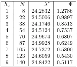
In this section we consider the scenario S1 and we assume
T = 25. We configure the window size such thatλ∗is maxi-mum under the constraintλ∗< T. We study the system for
hc= 1, . . . ,9 withc∈ K. The results are shown in Table 2 and the plot of ΦK as function ofhc is shown in Figure 2.
We can see that the fairness is improved by larger values of
hcbut, in order to control the maximum throughput, it re-quires larger windows and more memory. Hence, a trade-off between memory occupancy and desired fairness arises.
4.3
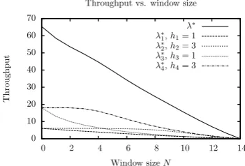
Different priority traffic streams
In this part we study a scenario in which we consider two pairs of streams 1,2 and 3,4 in a setting with the following packet generation rates
(6.0,6.0,18.0,18.0,3.8,1.2,1.5,1.72,1.12,8.0).
Streams 1 and 2 (resp. 3 and 4) have the same rates but the priority of 2 (resp. 4) is higher than that of 1 (resp. 3). We model this by settingh1=h3= 1 andh2=h4= 3. In
Fig-ure 4 we show the throughput of the four streams together with the total throughput. We notice that while with the increasing of the control window’s size the total throughput obviously decreases, the reduction of the bandwidth assigned
hc N λ∗ Φ
1 8 24.2832 1.2786 2 22 24.5006 0.9897 3 38 24.1746 0.8513 4 54 24.5124 0.7537 5 70 24.9674 0.6807 6 87 24.9928 0.6249 7 105 24.7372 0.5800 8 123 24.6059 0.5430 9 140 24.8422 0.5117
Table 2: Impact ofhcon the fairness index
to the high priority traffic streams 2 and 4 is much slower than that experienced by the lower priority streams 1 and 3.
5.
RELATED WORK
We discuss the works related to our contribution in two steps. First, we compare our approach with other works which address the problem of congestion control in WSNs (with or without priorities). Secondly, we compare our theo-retical contribution in terms of CTMC analysis with respect to the literature.
0 10 20 30 40 50 60 70
0 5 10 15 20 25 30 35 40
λ
∗
Window sizeN
Total throughput vs. window size S1hc= 1,2
hc= 1
hc= 2
(a) Total admission rate.
0 5 10 15 20
0 5 10 15 20 25 30 35 40
Throughput
Window sizeN
Throughput vs. window size S1hc= 1,2
λ∗
1,hc= 1
λ∗
20,hc= 1
λ∗
1,hc= 2
λ∗
20,hc= 2
(b) Admission rate of the slowest and fastes class.
0 0.2 0.4 0.6 0.8 1 1.2 1.4
0 5 10 15 20 25 30 35 40
F
airness
index
Window sizeN
Fairness index vs. window size S1hc= 1,2
ΦK,hc= 1 ΦK,hc= 2
(c) Fairness index.
Figure 1: Performance in Scenario 1 withhc= 1,2
0.5 0.6 0.7 0.8 0.9 1 1.1 1.2 1.3
1 2 3 4 5 6 7 8 9
F
airness
index
Φ
hc Fairness index vs.hcS1
Φ
Figure 2: Fairness as function ofhc
0 10 20 30 40 50 60
0 5 10 15 20 25 30 35 40
λ
∗
Window sizeN
Total throughput vs. window size S2hc= 1,2
hc= 1
hc= 2
(a) Total admission rate.
0 1 2 3 4 5 6 7
0 5 10 15 20 25 30 35 40
Throughput
Window sizeN
Throughput vs. window size S2hc= 1,2
λ∗
1,hc= 1
λ∗
20,hc= 1
λ∗
1,hc= 2
λ∗
20,hc= 2
(b) Admission rate of the slowest and fastes class.
0 0.5 1 1.5 2 2.5 3
0 5 10 15 20 25 30 35 40
F
airness
index
Window sizeN
Fairness index vs. window size S2hc= 1,2
ΦK,hc= 1 ΦK,hc= 2
(c) Fairness index.
Figure 3: Performance in Scenario 2 withhc= 1,2
0 10 20 30 40 50 60 70
0 2 4 6 8 10 12 14
Throughput
Window sizeN Throughput vs. window size
λ∗
λ∗
1,h1= 1
λ∗
2,h2= 3
λ∗
3,h3= 1
λ∗
4,h4= 3
customers. The authors propose a model for the analysis of
back-CHOKewhich is based on maintaining a window with the latestN packets arrived at the bottleneck. The packets coming from a source which is present in the window are discarded. Packet arrivals occur according to independent homogeneous Poisson processes, i.e., the model is a continu-ous time version of King’s model for the FIFO cache under the Independence Reference Model assumption (IRM) [13]. With respect to these papers, we propose a more sophisti-cated model in which the window may contain a number of replicas that depends on the traffic type. Moreover, we give an efficient algorithm to compute the performance measures that implements a convolution on the finite state space of the CTMC. Indeed, the algorithm developed in [7] is not applicable to our model due to the possible presence of du-plicated items in the window. Finally, with respect to the models studied in [13, 7, 16], we relax the requirements of the IRM by allowing the rate of the Poisson processes gener-ating the data at the motes to depend on the window state.
6.
CONCLUSION
In this paper we have proposed an allocation control sche-me, named FACW, for the bandwidth assignment in WSNs. The FACW protocol is easy to implement, consumes few re-sources in the motes and does not require extra control traf-fic in the WSN. We showed that it is able to handle traftraf-fic streams with different priorities and can reach a good level of fairness among streams with the same priority. Its main idea consists in maintaining at each mote a window with the lat-est traffic types perceived and dropping packets of the types that have reached their maximum population in the window. Under the assumption of Poisson generated traffic, we have proposed a model which is analytically tractable and gave an algorithm to efficiently derive the performance indices. The model extends previous ones such as those developed for studying FIFO caches [13] and back-CHOKe [16] in two directions: it allows for multiple entries of the same object in the window (allowing to control the priority of the traffic streams), and it considers that the traffic generation rate may depend on the state of the window at a certain epoch. Future works include providing an implementation of the protocol and performing simulations to assess the perfor-mance under more general scenarios.
7.
REFERENCES
[1] I. F. Akyildiz and I. H. Kasimoglu. Wireless sensor and actor networks: research challenges.Ad Hoc Networks, 2(4):351 – 367, 2004.
[2] D. Bertsekas and R. Gallager.Data networks. Prentice Hall, 1992.
[3] M. Caccamo, L. Zhang, S. Lui, and G. Buttazzo. An implicit prioritized access protocol for wireless sensor networks. InProc. of 23rd IEEE Real-Time Systems Symposium (RTSS), pages 39–48, 2002.
[4] M. Cherian and T. R. G. Nair. Priority based bandwidth allocation in wireless sensor networks.Int. J. of Computer Networks & Communications
(IJCNC), 6(6):119–128, 2014.
[5] M. Chitnis, P. Pagano, G. Lipari, and Y. Liang. A survey on bandwidth resource allocation and scheduling in wireless sensor networks. InProc. of
IEEE Int. Conf. on Network-Based Information Systems, pages 121–128, 2009.
[6] C. T. Ee and R. Bajcsy. Congestion control and fairness for many-to-one routing in sensor networks. In
Proc. of the 2Nd Int. Conf. on Embedded Networked Sensor Systems, pages 148–161, 2004.
[7] R. Fagin and T. G. Price. Efficient calculation of expected miss ratios in the independent reference model.SIAM J. Comput., 7(3):288–297, 1978. [8] E. L. Hahne. Round-robin scheduling for max-min
fairness in data networks.IEEE Journal on Selected Areas in Communications, 9:1024–1039, 1991.
[9] Z. Hanzalek and P. Jurˆcik. Energy efficient scheduling for cluster-tree wireless sensor networks with
time-bounded data flows: Application to ieee 802.15.4/zigbee.Industrial Informatics, IEEE Transactions on, 6(3):438 – 450, Aug 2010. [10] T. He, J. A. Stankovic, C. Lu, and T. Abdelzaher.
SPEED: A stateless protocol for real-time communication in sensor networks. InProc. 23rd IEEE Int. Conf. on Distributed Computing Systems, pages 46–55, 2003.
[11] F. Kelly.Reversibility and stochastic networks. Wiley, New York, 1979.
[12] D. Khan, B. Nefzi, L. Santinelli, and Y. Song. Probabilistic bandwidth assignment in wireless sensor networks. InWireless Algorithms, Systems, and Applications, volume 7405 ofLecture Notes in Computer Science, pages 631–647. Springer Berlin / Heidelberg, 2012.
[13] W. F. King. Analysis of paging algorithms. InProc. of IFIP Congr., 1971.
[14] A. Marin and S. Rossi. On discrete time reversibility modulo state renaming and its applications. InProc. of Valuetools 2014, 2014.
[15] A. Marin and S. Rossi. On the relations between lumpability and reversibility. InProc. of the IEEE 22nd Int. Symp. on Modeling, Analysis and Simulation of Computer and Telecommunication Systems (MASCOTS’14), pages 427–432, 2014. [16] R. Pan, B. Prabhakar, and K. Psounis. CHOKe, A
stateless active queue management scheme for approximating fair bandwidth allocation. InProc. of IEEE INFOCOM ’00, pages 942–951, Washington, DC, 2000. IEEE Computer Society Press.
[17] Y. Sankarasubramabiam, O. Akan, and I. Akyildiz. Event-to-sink reliable transport in wireless sensor networks. InProc. of the 4th ACM Symposium on Mobile Ad Hoc Networking & Computing, MobiHoc, pages 177–188, 2003.
[18] C. Wan, S. B. Eisenman, and A. T. Campbell. Coda: Congestion detection and avoidance in sensor networks. InFirst ACM Conf. on Embedded Networked Sensor Systems, pages 266–279, 2003. [19] P. Whittle.Systems in stochastic equilibrium. John
Wiley & Sons Ltd., 1986.