Modelling the Spatial and Temporal Change in Diffusion Rates of Molasses in Sand Medium

Malaysian Journal of Soil Science Vol. 13: 93-104 Malaysian Society of Soil Science

Modelling the Spatial and Temporal Change in Diffusion

Rates of Molasses in Sand Medium

E.G. Goh & I. Athira

Department of Engineering Science, Faculty of Science and Technology,

Universiti Malaysia Terengganu, Mengabang Telipot,

21030 Kuala Terengganu, Terengganu, Malaysia

INTRODUCTION

In natural environment, there is spatial imbalance in distribution of natural substances in terms of concentration. However, eventually any differences in concentration at separate locations will naturally be levelled off in time. This natural phenomenon is known as diffusion. Diffusion from the physical point of view is basically the result of random movement of molecule. This random movement is a function of temperature, and hence, increasing temperature would increase the speed of random movement.

Mass flux rate (kg s-1_{) through a unit area (m}2_{) due to molecular diffusion is} correlated to concentration gradient with a constant D that is known as diffusion coefficient (m2 _s-1_{). This relationship is described by first Fick’s law as follows} (Demonico and Schwartz, 1990):

ABSTRACT

Diffusion is one of the important parameters in groundwater study. In a relatively slow moving groundwater, diffusion could be a dominant factor in transporting contaminants between liquid-solid interface and liquid-liquid interchange. The diffusion coefficient of dissolved substance is normally tabulated as a constant value, irrespective of the influence of space and time. In this study, molasses was taken as a dissolved organic carbon (DOC) representation, and it was injected into a basin filled with porous medium (sand) in which it was allowed to diffuse horizontally and vertically in space and time. Diffusion coefficient was determined from first and second Fick’s law, in which the later model was solved with polynomial equation. Diffusion coefficient was observed with respect to changes in space and time. A large fluctuation of diffusion coefficient was more apparent at the initial stage of diffusion. Changes of DOC concentration eventually stabilized after a longer time period. Diffusion coefficient from second Fick’s law was found to be more informative than the first Fick’s law. From graphical observation, four types of concentration-distant relation curve were proposed to classify an observed relation of concentration and distant.

Keywords: molasses, dissolved organic carbon, diffusion coefficient, Fick’s

(1)

where x is the horizontal distance (m), F is the mass flux rate per unit area (kg m-2 s-1_{) and C is solute concentration (kg m}-3_).

The transport of a chemical substance from a higher concentration to lower concentration region is a continuous process. Hence, the difference of concentration between locations will also vary with time. This suggests that Eq. (1) only modelled diffusion mechanism at a specific time. In order to model diffusion for both distant and time, second Fick’s law was used as follows (Appelo and Postma, 2005):

(2)

where t is for time (s).

Diffusion is one of the few important mechanisms in governing contaminant transport in groundwater. For instance, there are mechanical dispersion, degradation, adsorption, and advection. In groundwater modelling software, for example, SUTRA program on solute transport in subsurface system employed diffusion as a constant input parameter (Voss and Provost 2003). Diffusion is influenced by various factors such as water content, compaction on soils, porosity distribution, types of chemical substance (hydrophilic, hydrophobic, anion, cation, etc), and tortuosity (Mott and Weber 1991; Shackelford and Daniel 1991; Myrand

et al. 1992; Cotten et al. 1998). The current work was limited to spatial and time factors, which was based on Eq. (2).

Arsenic pollution in the groundwater of east and west Bengal is a well-known problem. Study from Islam et al. (2004) had shown that simultaneous organic carbon oxidation and reduction of arsenic-bearing Fe(III) compounds may be implicated with the release of arsenic from sediment to groundwater. The availability of organic matter either from surface-derived infiltration or naturally embedded in sediment with a slow release from sediment, or a combination of both has an important implication in the management of arsenic contamination in groundwater. In this context, diffusion coefficient has an important practical contribution on the movement of organic mass from sediment or ground surface into groundwater.

The objectives of this work were to: (1) solve second Fick’s law using polynomial equations; and (2) illustrate and classify diffusion phenomenon into different types of Concentration (C)-Distant (x) relation. In this study, molasses was used as a representation of natural organic matter. Molasses-induced arsenic in groundwater was observed in the work of Harvey et al. (2002) in east Bengal. Other workers chose to use acetate to induce arsenic release from sediment (Van Geen et al. 2004; Coker et al. 2006; Lear et al. 2007).

x C D F

MATERIALS AND METHODS

Experimental Setting

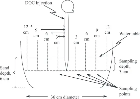
Sand was collected from a seaside of Kuala Terengganu, Terengganu, Malaysia, and the sand was subjected to a sieving machine in which it consisted of sieve sizes ranging from 0.063 μm to 4.0 mm. Sand ranging from 0.43 to 2.0 mm (medium to very coarse sand, respectively) was chosen to allow reasonable measurement of solute diffusion process in the timeframe of laboratory experimentation. This is because smaller sand size would decrease the diffusion process which would eventually require a longer period of experimentation, and vice versa for a larger sand size. A diffusion testing model was constructed as shown in Fig. 1. A basin of 36 cm was filled with 6 cm depth of sand and then, filled with demineralised water until it was slightly above the surface of sand. Dissolved organic carbon (DOC) was represented by molasses (C₆H₁₂NNaO₃S) and was prepared to a concentration of 30 mg L-1_{. The DOC was injected into the sand at 3 cm below} the water table in the middle of the basin. For every 15 minutes, water sample was collected at 3 cm depth from horizontal distance of 3, 6, 9, and 12 cm from the injection point. The concentration of DOC was measured with a TOC-V_CPH Shimadzu Analyzer in triplicates. An average value was calculated and was used for graphical illustration as well as the determination of diffusion coefficients in first and second Fick’s law.

Fig. 1: A diffusion model testing unit on porous medium.

(3)

(4)

(5)

where:

1 1,t

x

C is the concentration (mg L-1_{) at x}

1 distance from injection point at time t₁ ;

1 2,t

x

C is the concentration (mg L-1) at x2 distance from injection point at time t₁;

2 2,t

x

C is the concentration (mg L-1_{) at x}

2 distance from injection point at time t₂ ; and and x₁ < x₂and t₁ < t₂

Eq. (4) was proposed to approximate Eq. (3), and it can be reduced to Eq. (5). From Eq. (4), its numerator denotes mass flux rate per unit area and denominator denotes concentration gradient. The numerator was derived from the following equation:

where:

.

m

Mathematical Solution to the Diffusion Coefficient of the Second Fick’s Law Diffusion coefficient of second Fick’s law was calculated at discrete location from 3 to 12 cm and at discrete time from 0 to 120 minutes. Polynomial equations were used to correlate concentration (C) of DOC with time (t) and DOC travel distant (x) as shown below:

(6)

(7)

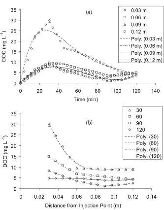
where: a_t, a_x, b_t, b_x, c_t, c_x, d_t, d_x, e_t, and f_t are coefficients of polynomial equations. The fitted curves and standard deviation on experimental data are shown in Figs. 2(a) and 2(b), respectively, generated from Eqs. (6) and (7).

In order to avoid a possible unwanted generation of “bump” in the curve prediction, linear interpolation between experimental data was carried out to estimate data points and these data were used in the curve-fitting, as shown in Figs. 2(a) and 2(b).

(

) (

)

(

) ( )

( )

A m

F_{= = ×} 1 _{× = × = ×}

.

.

Fig. 2: Curve-fitting results: (a) the correlation between concentration (C) and time (t) which has the lowest R2 _{from 0.936. The plotted DOC data in-between 0, 15, 30,} 45, 60, 75, 90, 105 and 120 min were generated from linear interpolation; and (b) the

correlation between concentration (C) and distant (x) which has the lowest R2 _from 0.934. The plotted DOC data in-between 0.03, 0.06, 0.09 and 0.12 m were generated

from linear interpolation.

Note that a minimum requirement of estimation on any equation parameters is to have a number of experimental data equal or more than the number of parameter required to be estimated from proposed equation. In the current study,

0 5 10 15 20 25 30 35

0 20 40 60 80 100 120 140

Time (min) D O C ( m g L -1 ) 0.03 m 0.06 m 0.09 m 0.12 m Poly. (0.03 m) Poly. (0.06 m) Poly. (0.09 m) Poly. (0.12 m)

0 5 10 15 20 25 30 35

0 0.02 0.04 0.06 0.08 0.1 0.12 0.14

Distance from Injection Point (m)

Eq. (6) with six equation parameters was estimated by nine experimental data and combined fitted to additional twenty four interpolated data, and Eq. (7) with four parameters was estimated by four experimental data and combined fitted to additional nine interpolated data. Hence, the orders of polynomial used in the study are considered reasonable.

By taking the derivative of C with respect to t , and second derivative of C

with respect to x, they become the following forms:

(8)

(9)

The diffusion coefficient of second Fick’s law can be solved by rearranging Eq. (2) and then, employ solution from Eqs. (8) and (9). The solution is shown below:

(10)

(11)

Eq. (11) is not intended as an ultimate analytical equation in solving for the diffusion coefficient of second Fick’s law, but it was rather proposed as one of the easiest and practical solution in achieving the first objective of the current work.

RESULTS AND DISCUSSION

DOC Diffusion in Space and Time

Immediately after the injection of DOC (molasses) into the middle of the basin in which it was filled with sand and demineralised water, there was a distinctive region of high and low (or very low) DOC concentration. As time increased, DOC became increasingly uniform throughout the system (Fig. 3).

Overall, diffusion had created regions in which there were the highest and the lowest concentration regions of DOC. However, after a longer time of diffusion (approximately at 120 minutes), a levelling off of DOC concentration for all locations was observed which ranged from 3.8 to 4.9 mg L-1 _{with a} standard deviation of 0.5 mg L-1_{. At this region the system was approximating a} homogenous DOC concentration distribution. Further evaluation was carried out with the determination of diffusion coefficient from the first and second Fick’s law.

Fig. 3: Concentration of molasses in porous medium in space and time.

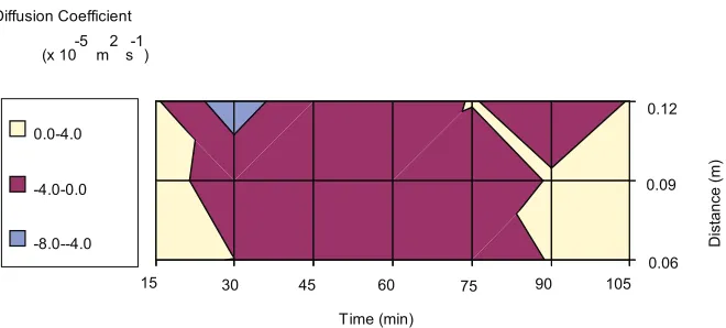
Fig. 4. Diffusion coefficient of molasses in porous medium in space and time which was calculated from first Fick’s law.

Time (min) Diffusion Coefficient

(x 10-5 m2 s-1)

0.0-4.0

-4.0-0.0

-8.0--4.0 Distance (m)

0.09 0.12

0.06 15 30 45 60 75 90 105 DOC (mg L-1)

26.6-30.4

22.8-26.6

19.0-22.8

15.2-19.0

11.4-15.2

7.6-11.4

3.8-7.6

0.0-3.8

Distance from injection

point (m)

Time (min)

0 15 30 45 60 75 90 105 120

Diffusion Coefficient of the First Fick’s Law

Diffusion coefficient determined from the first Fick’s law can be broadly

categorized into those of positive and negative values. A positive value of the

diffusion coefficient is referring to DOC flux that is diffusing away from the

injection point, and the DOC concentration is increasing with increasing time.

A positive value could also be given by DOC flux that is diffusing towards

injection point, and the DOC concentration is decreasing with increasing time. A

negative diffusion coefficient indicates DOC flux that is diffusing away from the

injection point, and the DOC concentration is decreasing with increasing time.

Alternatively, negative diffusion coefficient could also indicate DOC flux that is

diffusing towards the injection point, and the DOC concentration is increasing with increasing time.

It is observed that within the two hours of diffusion, the initial and the last

15 minutes have given positive values of diffusion coefficients (Fig. 4), whereas in between it was dominated by negative diffusion coefficients. At 12 cm and 30 minutes, a large magnitude of negative diffusion coefficient was found as - 6.6 x

10-5 _m2 _s-1. _{This is because of a smaller concentration gradient that was required to}

cause a larger amount of DOC flux, which could be due to the non-homogeneous

distribution of sand. The following diffusion coefficients of D_12cm,75mins, D_9cm,90mins

and D_6cm,90mins where a sudden change of sign in diffusion coefficients was indicated.

This was due to a change in solute mass accumulation from DOC concentration that decreases with increasing time to DOC concentration which increases with increasing time. Diffusion at 12 cm and 90 minutes was a result of reversal in

solute mass transport direction that was diverted from DOC flux which diffuses away from injection point to DOC flux which diffuses towards the injection

point.

Diffusion Coefficient of the Second Fick’s Law

Similar to first Fick’s law, the diffusion coefficient determined from second Fick’s law also can be broadly divided into those of positive and negative values. However, it has more characteristics than the diffusion coefficient of the first Fick’s

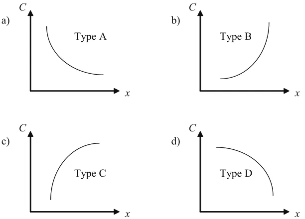
law, and thus, it carries more information. As a result, four graphical illustration as

shown in Fig. 5 is proposed to categorize the observation of experimental results. Since the second Fick’s law accounted for both space and time, the positive value of diffusion coefficient indicates an increasing DOC concentration with time, and

DOC flux is diffusing either towards or away from injection point with C - x

curve concaves upwards. Also, a positive value could indicate a decreasing DOC

concentration with time, and DOC flux is diffusing either towards or away from

injection point with C - x curve concaves downwards. For negative value of

diffusion coefficient, the DOC concentration is increasing with time, and DOC

flux is diffusing either towards or away from injection point with C - x curve

concaves downwards. Alternatively, negative could be due to decreasing DOC

concentration with time, and DOC flux is diffusing either towards or away from

Fig. 5: Types of C - x curve: (a) Decreasing DOC concentration with distant (concave upwards); (b) Increasing DOC concentration with distant (concave upwards); (c) Increasing DOC concentration with distant (concave downwards); and (d) Decreasing

DOC concentration with distant (concave downwards).

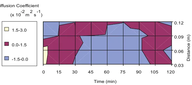
At the initial stage of diffusion, between 0 and 15 minutes, a large fluctuation of diffusion coefficients was observed from 3 to 12 cm (Fig. 6). This observation deviates from the diffusion coefficient that was determined from first Fick’s law. This could be explained by the method of calculation proposed in Eq. (5) in which its diffusion coefficient is subjected to the influence of adjacent concentration

in subsequent time of diffusion. As a result, the estimated value was unable to

illustrate a definite change of diffusion coefficient, and also subjected to limitation in the availability of experimental data.

As shown in Fig. 6, the first 30 minutes of diffusion has given a positive

diffusion coefficient, except at D_3cm,30mins, D_9cm,0mins and D_{12cm,0-30mins}. This region has

shown a dominant increasing (or accumulating) DOC concentration with time,

which was an indication of DOC flux from high concentration to low concentration

regions.

The region from 45 to 90 minutes has diffusion coefficient in negative value,

except at D_{12cm,45-90mins}. This region was governed by diffusion in which its DOC

concentration decreases with increasing time and the DOC flux was diffusing

away from the injection point. A decreasing DOC concentration during diffusion is an indication of mass dispersion that would lead towards a homogenous DOC concentration.

a)

x C

b)

x C

x C

d)

x C

c)

Type A

Type C

Type B

Fig. 6: Diffusion coefficient of molasses in porous medium in space and time, calculated from second Fick’s law.

From 105 to 120 minutes, it was found mainly positive diffusion coefficient,

except at D_6cm,120mins and D_12cm,120mins. Also, it has half of its DOC flux diffuses

towards the injection point and approximately, half of its diffusion with DOC

concentration increases with increasing time. The balance of back and forward

of DOC flux that either diffuses towards or away from the injection point and

with the balance of increasing and decreasing DOC concentration with time, these observations could be used to indicate the onset of diffusion system stabilization in which it showed a lower DOC concentration (Fig. 3) and a lower diffusion

coefficient with less fluctuation in values.

An average diffusion coefficient of 1.2 x 10-2 _m2 _s-1 _{(± 9.3 x 10}-3_{) at 0 minute,}

it gradually decreases to an average of 1.1 x 10-4 _m2 _s-1 _{(± 7.4 x 10}-5_{) at 120}

minutes. At 0 minute, diffusion coefficient was the highest with respective 1.9 x

10-2 _{and 2.1 x 10}-2 _{m2 s}-1 _{at 3 and 6 cm. This was caused by a high concentration}

gradient that generates greater DOC flux at the early stage of DOC injection. A

negative diffusion coefficient of D_9cm,0mins and D_{12cm,0-30mins} was due to its respective

types C and D (concaves downwards) of C- x curves which generates negative value on the second derivative of C with respect to x (i.e., d2_C/dx2_{= -1 ) (see Fig.} 5). For D_3cm,30mins, and D_12cm,120mins, the negative diffusion coefficient was due to the decreasing DOC flux with time which generates negative value on concentration

rate (i.e., dC/dt = -1 ), whereas at D_6cm,120mins it was caused by its type D of C - x

curves.

CONCLUSIONS

Diffusion of molasses in porous medium (sand) dynamically varies in space and

time. The fluctuation of DOC concentration in space and time causes fluctuation of diffusion coefficient which was apparently observed from the calculated diffusion coefficient obtained from second Fick’s law. The injected DOC has gone through

a rapid random motion which causes a quick jump in DOC concentration at the initial 30 minutes of diffusion and gradually decreasing the DOC concentration in

0 15 30 45 60 75 90 105 120

0.03 0.06 0.09 0.12 Diffusion Coefficient

(x 10-2 m2 s-1)

1.5-3.0

0.0-1.5

-1.5-0.0 Distance (m)

the remaining time, before stabilizing at the last 15 to 30 minutes of diffusion. The proposed four types of C - x curve appeared sufficient in classifying the relation of

concentration and distant from the injection point. Types A and D were the most dominant C - x curves in the current laboratory scale diffusion system and it is

limited to the observation of 120 minutes and to a maximum of 12 cm observation

distance from the injection point.

REFERENCES

Appelo, C.A.J. and D. Postma. 2005. Geochemistry, groundwater and pollution. 2nd edn.

A.A. Balkema Publisher, Laiden.

Coker V.S., A.G. Gault, C.I. Pearce, G. van der Laan, N.D. Telling, J.M. Charnock, D.A. Polya and J.R. Lloyd. 2006. XAS and XMCD evidence for species-dependent partitioning of arsenic during microbial reduction of ferrihydrite to magnetite.

Environ Sci Technol.40: 7745-7750.

Cotten, T.E., M.M. Davis and C.D. Shackelford. 1998. Effects of test duration and specimen

length on diffusion testing of unconfined specimens. Geotechnical Testing Journal.21: 79-94.

Domenico, P.A. and F.W. Schwartz. 1990. Physical and Chemical Hydrogeology. John Wiley and Sons, Inc., Canada.

Harvey, C.F., C.H. Swartz, A.B.M. Badruzzaman, N. Keon-Blute, W. Yu, M.A. Ali, J. Jay, R. Beckie, V. Niedan, D. Brabander, P.M. Oates, K.N. Ashfaque, S. Islam, H.F. Hemond, and M.F. Ahmed. 2002. Arsenic Mobility and Groundwater Extraction in Bangladesh. Science.298: 1602-1606.

Islam, F.S., A.G. Gault, C. Boothman, D.A. Polya, J.M. Charnock, D. Chatterjee and J.R. Lloyd. 2004. Role of metal-reducing bacteria in arsenic release from Bengal delta

sediments. Nature. 430: 68-71.

Lear G., B. Song, A.G. Gault, D.A. Polya and J.R. Lloyd. 2007. Molecular analysis of

arsenate-reducing bacteria within Cambodian sediments following amendment with acetate. Appl Environ Microbiol. 73:1041–1048.

Mott, H.V. and W.J. Weber. 1991. Factors influencing organic contaminant diffusivities in

soil-bentonite cutoff barriers. Environmental Science and Technology. 25: 1708-715.

Myrand, D., R.W. Gillham, E.A. Sudicky, S.F. O’Hannesin and R.L. Johnson. 1992.

Diffusion of volatile organic compounds in natural clay deposits: laboratory tests.

Journal of Contaminant Hydrology. 10: 159-177.

Van Geen, A., J. Rose, S. Thoral, J.M. Garnier, Y. Zheng and J.Y. Bottero. 2004. Decoupling of As and Fe release to Bangladesh groundwater under reducing conditions. Part

II: Evidence from sediment incubations. Geochem Cosmochem Acta. 68: 3475-3486.