Resampling-Based Ensemble Methods for Online Class Imbalance Learning

Resampling-Based Ensemble Methods for

Online Class Imbalance Learning

Shuo Wang,

Member, IEEE,

Leandro L. Minku,

Member, IEEE,

and Xin Yao,

Fellow, IEEE

Abstract—Online class imbalance learning is a new learning problem that combines the challenges of both online learning and class imbalance learning. It deals with data streams having very skewed class distributions. This type of problems commonly exists in real-world applications, such as fault diagnosis of real-time control monitoring systems and intrusion detection in computer networks. In our earlier work, we defined class imbalance online, and proposed two learning algorithms OOB and UOB that build an ensemble model overcoming class imbalance in real time through resampling and time-decayed metrics. In this paper, we further improve the resampling strategy inside OOB and UOB, and look into their performance in both static and dynamic data streams. We give the first comprehensive analysis of class imbalance in data streams, in terms of data distributions, imbalance rates and changes in class imbalance status. We find that UOB is better at recognizing minority-class examples in static data streams, and OOB is more robust against dynamic changes in class imbalance status. The data distribution is a major factor affecting their performance. Based on the insight gained, we then propose two new ensemble methods that maintain both OOB and UOB with adaptive weights for final predictions, called WEOB1 and WEOB2. They are shown to possess the strength of OOB and UOB with good accuracy and robustness.

Index Terms—Class imbalance, resampling, online learning, ensemble learning, Bagging.

F

1

I

O

topic that is attracting growing attention. It aims to tackle the combined issue of online learning [1] and class imbalance learning [2]. Different from incre-mental learning that processes data in batches, online learning here means learning from data examples “one-by-one” without storing and reprocessing ob-served examples [3]. Class imbalance learning handles a type of classification problems where some classes of data are heavily underrepresented compared to other classes. With both problems, online class imbalance learning deals with data streams where data arrive continuously and the class distribution is imbalanced. Although online learning and class imbalance learn-ing have been well studied in the literature individ-ually, the combined problem has not been discussed much. It is commonly seen in real world applications, such as intrusion detection in computer networks and fault diagnosis of control monitoring systems [4].

When both issues of online learning and class imbalance exist, new challenges and interesting re-search questions arise, with regards to the predic-tion accuracy on the minority class and adaptivity to dynamic environments. The difficulty of learning from imbalanced data is caused by the relatively or absolutely underrepresented class that cannot draw

• The authors are with the Centre of Excellence for Research in Compu-tational Intelligence and Applications (CERCIA), School of Computer Science, The University of Birmingham, Edgbaston, Birmingham B15 2TT, UK. E-mail:{S.Wang, L.L.Minku, X.Yao}@cs.bham.ac.uk

equal attention to the learning algorithm compared to the majority class. It often leads to very specific classification rules or missing rules for the minority class without much generalization ability for future prediction [5]. This problem is exaggerated when data arrive in an online fashion. First, we cannot get a whole picture of data to evaluate the imbalance status. An online definition of class imbalance is necessary to describe the current imbalance degree. Second, the imbalance status can change over time. Therefore, the online model needs to be kept updated for good performance on the current minority class without damaging the performance on the current majority class.

accuracy measured byG-mean [6].

However, because the resampling rate in OOB and UOB does not consider the size ratio between classes, there exists an issue that the resampling rate is not consistent with the imbalance degree in data and varies with the number of classes. Besides, no existing work has studied the fundamental issues of class imbalance in online cases and the adaptivity of online learners to deal with dynamic data streams with a varying imbalance rate so far. Most work focuses on online learning with concept drifts that involve classification boundary shifts. This paper will give the first comprehensive analysis of class imbalance in data streams.

First, we improve the resampling setting strategies in OOB and UOB. Second, we look into the perfor-mance of improved OOB and UOB in both static and dynamic data streams, aiming for a deep under-standing of the roles of resampling and time-decayed metrics. We also give a statistical analysis of how their performance is affected by data-related factors and al-gorithm settings through factorial ANOVA. Generally speaking, our experiments show the benefits of using resampling and time-decayed metrics in the improved OOB and UOB. Particularly, UOB is better at recog-nizing minority-class examples in static data streams, and OOB is more robust against dynamic changes in class imbalance status. The data distribution is a major factor affecting their performance.

Based on the achieved results, for better accuracy and robustness under dynamic scenarios, we propose two ensemble strategies that maintain both OOB and UOB with adaptive weight adjustment, called WEOB1 and WEOB2. They are shown to successfully combine the strength of OOB and UOB. WEOB2 outperforms WEOB1 in terms of G-mean.

2

L

I

D

S

In this section, we define class imbalance under online scenarios, introduce the two classification methods (i.e. OOB and UOB), and review the research progress in learning from imbalanced data streams. They form the basis of this paper.

2.1 Defining Class Imbalance

To handle class imbalance online, we first need to define it by answering the following three questions: 1) is the data stream currently imbalanced? 2) Which classes belong to the minority/majority? 3) What is the imbalance rate currently? We answered the ques-tions by defining two online indicators – time-decayed class size and recall calculated for each class [6]. Different from the traditional way of considering all observed examples so far equally, they are updated incrementally by using a time decay (forgetting) factor to emphasize the current status of data and weaken the effect of old data.

Suppose a sequence of examples (xt, yt) arriving one at a time.xtis a p-dimensional vector belonging to an input space X observed at time t, and yt is the corresponding label belonging to the label set

Y = {c1, . . . , cN}. For any class ck ∈ Y, the class size indicates the occurrence probability (percentage) of examples belonging tock. If the label set contains only two classes, then the size of the minority class is referred to as the imbalance rate (IR) of the data stream, reflecting how imbalanced the data stream is at the current moment. The recall of classck indicates the classification accuracy on this class. To reflect the current characteristics of the data stream, these two indicators are incrementally updated at each time step. When a new examplextarrives, the size of each class, denoted byw(_kt), is updated by [6]:

w_k(t)=θw_k(t−1)+ (1−θ) [(xt, ck)],(k= 1, . . . , N) (1) where [(xt, ck)] = 1 if the true class label of xt is

ck, otherwise 0. θ (0< θ <1) is a pre-defined time decay factor, which forces older data to affect the class percentage less along with time through the exponential smoothing. Thus, w(_kt) is adjusted more based on new data.

Ifxt’s real labelytisci, the recall of classci, denoted byR(_it), is updated by [6]:

R(_it)=θ0R_i(t−1)+ (1−θ0) [xt←ci]. (2) For the recall of the other classes, denoted by R(_jt)

(j6=i), it is updated by:

R(_jt)=R_j(t−1),(j= 1, . . . , N, j6=i). (3) In Eq.2, θ0 (0< θ0<1) is the time decay factor for emphasizing the learner’s performance at the cur-rent moment. [xt←ci] is equal to 1 if x is correctly classified, and 0 otherwise. θ = 0.9 and θ0 = 0.9 were shown to be a reasonable setting to balance the responding speed and the estimation variance in our experiments [6].

w(t)andR(t)values are then used by a class imbal-ance detection method, which outputs the information of whether the data stream should be regarded as imbalanced and which classes should be treated as the minority class. It examines two conditions for any two classesci andcj:

• wi−wj > δ1 (0< δ1<1)

• Ri−Rj> δ2 (0< δ2<1)

If both conditions are satisfied, then classcj is sent to the minority class label set Ymin and class ci is sent to the majority class label setYmaj. IfYmin and

because it has been agreed that the imbalance rate is not the only factor that causes the classification diffi-culty [8]. There are easy cases where both minority-and majority-class recall values are quite high minority-and resampling is not necessary, such as linearly separable problems; there are also difficult cases where the recall difference between minority and majority classes is high due to the performance trade-off [9], such as data with overlapping [10] [11] and small disjuncts [12].

2.2 Online Solutions OOB and UOB

With the information from the class imbalance detec-tion method, we proposed OOB and UOB to learn im-balanced data streams [6]. They integrate resampling into ensemble algorithm Online Bagging (OB) [7]. Resampling is one of the simplest and most effective techniques of tackling class imbalance [13] [14]. It works at the data level independently of the learning algorithm. Two major types of resampling are over-sampling – increasing the number of minority-class examples, and undersampling – reducing the number of majority-class examples. Online Bagging [7] is an online ensemble learning algorithm that extends the offline Bagging [15]. It builds multiple base classi-fiers and each classifier is trained K times by using the current training example, where K follows the

P oisson(λ= 1) distribution. Poisson distribution is used, because the Binomial distribution K in offline Bagging tends to the Poisson(1) distribution when the bootstrap sample size becomes infinity.

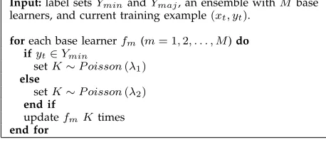
OnceYminandYmaj (the output of the class imbal-ance detection method) are not empty, oversampling or undersampling embedded in Online Bagging will be triggered to either increase the chance of train-ing minority-class examples (in OOB) or reduce the chance of training majority-class examples (in UOB). Their training procedures are given in Table 1.

TABLE 1: OOB and UOB Training Procedures.

Input:label setsYminandYmaj, an ensemble withM base

learners, and current training example(xt, yt).

foreach base learnerfm(m= 1,2, . . . , M)do

ifyt∈Ymin

setK∼P oisson(λ1)

else

setK∼P oisson(λ2)

end if

updatefmKtimes

end for

Resampling in OOB and UOB is performed through the parameterλof Poisson distribution to handle class imbalance. In OOB, λ1 is set to 1/w

(t)

k ; λ2 is set to 1. In UOB, λ1 is set to 1, λ2 is set to

1−w_k(t). If the new training example belongs to the minority class, OOB increases value K, which decides how many times to use this example for training. Similarly,

if it belongs to the majority class, UOB decreases

K. The advantages of OOB and UOB are: 1) the class imbalance technique (resampling) is algorithm-independent, which allows any type of online clas-sifiers to be used; 2) time-decayed class size used in OOB and UOB dynamically estimates imbalance status without storing old data or using windows, and adaptively decides the resampling rate at each time step, which enlarges their learning adaptivity under nonstationary environments; 3) like other ensemble methods, they combine the predictions from multiple classifiers, which are expected to be more accurate than a single classifier.

2.3 Existing Research

Most existing algorithms dealing with imbalanced data streams require processing data in batches/chunks (incremental learning), such as MuSeRA [16] and REA [17] proposed by Chen et al., and Learn++.CDS and Learn++.NIE [18] proposed by Ditzler and Polikar. Among limited class imbalance solutions strictly for online processing, Nguyen et al. first proposed an algorithm to deal with imbalanced data streams through random undersampling [19]. The majority class examples have a lower probability to be selected for training. It assumes that the information of which class belongs to the minority/majority is known and the imbalance rate does not change over time. Besides, it requires a training set to initialize the classification model before learning. Minku et al. [20] proposed to use undersampling and oversampling to deal with class imbalance in online learning by changing the parameter corresponding to Online Bagging’s [7] sampling rate. However, the sampling parameters need to be set prior to learning and cannot be adjusted to changing imbalance rates. Very recently, two perceptron-based methods RLSACP [21] and WOS-ELM [22] were proposed, which assign different misclassification costs to classes to adjust the weights between perceptrons. The error committed on the minority class suffers a higher cost. RLSACP adopts a window-based strategy to update misclassification costs based on the number of examples in each class at a pre-defined speed. WOS-ELM requires a validation set to adjust misclassification costs based on classification performance, which however may not be available in many real-world applications. They were tested in static scenarios with a fixed imbalance rate and shown to be effective.

3

I

OOB

UOB

that, when the data stream becomes balanced,λwill not be equal to 1. It means that the resampling keeps running even when the data is balanced, if the class imbalance detection method is not applied as the trig-ger. For example, given a balanced 2-class problem, where w(_kt) is equal to 0.5, λ for one class will be set to 2 by OOB; given a balanced 5-class problem, where w_k(t) is equal to 0.2, λfor one class will be set to 5 by OOB. On the one hand, the strategy of setting

λ is not consistent with the imbalance degree, and varies with the number of classes. On the other hand, it is necessary to use the class imbalance detection method, to inform OOB and UOB of when resampling should be applied.

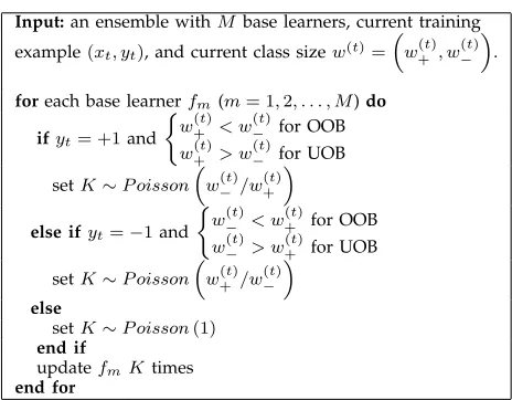
To overcome this issue, we improve OOB and UOB with a better parameter setting strategy in this section.

λin the improved versions is determined by the size ratio between classes. The pseudo-code of improved OOB and UOB at each training step t is given in Table 2, assuming there are two possible classes Y =

{+1,−1} (denoted by ‘+’ and ‘-’ for simplicity). TABLE 2: Improved OOB and UOB.

Input:an ensemble withM base learners, current training

example(xt, yt), and current class sizew(t)=

w(t)₊ , w(t)−

.

foreach base learnerfm(m= 1,2, . . . , M)do

ifyt= +1and

w(t)₊ < w(t)₋ for OOB

w(t)₊ > w(t)₋ for UOB

setK∼P oisson

w(t)₋/w₊(t)

else ifyt=−1and

w(t)− < w

(t)

+ for OOB

w(t)₋ > w(t)₊ for UOB setK∼P oisson

w(t)₊ /w−(t)

else

setK∼P oisson(1)

end if

updatefmKtimes

end for

Simply to say, if the size of the positive class is smaller than the size of the negative class at the current moment,λfor the positive class will be set to

w(₋t)/w(₊t)for oversampling in OOB;λfor the negative class will be set to w₊(t)/w₋(t) for undersampling in UOB. With the same Bagging strategy as the tradi-tional Online Bagging (OB) [7], improved OOB and UOB only sweep through each training example once, sent to all base classifiers. So, they need O(M) time to keep the online model up-to-date, when the base classifiers are updated sequentially.

When data become balanced, these methods will be reduced to OB automatically. For any 2-class prob-lems, therefore, it is not necessary to apply the class imbalance detection method any more for a hard par-tition of class labels into minority and majority label sets. For multi-class problems, however, this hard

par-tition is still necessary for choosing w(_mint) and w_maj(t) , where w(_mint) (w(maj) stands for the class size of thet) smaller (larger) class. For example, for a data stream with 4 classes{c1, c2, c3, c4}, their proportions are 0.05, 0.15, 0.25, 0.55 respectively. Classc3is a majority class relative toc1, but a minority class relative toc4. Since we do not want to overlook the performance of any minority class, the class imbalance detection method will labelc3as minority. This information is then used by OOB and UOB to treat this class. Without recogniz-ing this situation, it would be difficult to determine the way of sampling. This paper focuses on 2-class imbalanced data streams, so we do not use the class imbalance detection method to trigger resampling in improved OOB and UOB here. How it helps the classification in multi-class cases will be studied as our next-step work. All the following analysis will be based on the improved OOB and UOB. We will simply use “OOB” and “UOB” to indicate the improved ones for brevity.

4

C

I

A

S

D

S

This section studies OOB and UOB in static data streams without any changes. We focus on the fun-damental issue of class imbalance and look into the following questions under different imbalanced sce-narios: 1) to what extent does resampling in OOB and UOB help to deal with class imbalance online? 2) How do they perform in comparison with other state-of-the-art algorithms? 3) How are they affected by different types of class imbalance and classifiers? For the first question, we compare OOB and UOB with OB [7], to show the effectiveness of resampling. For the second question, we compare OOB and UOB with two recently proposed learning algorithms, RL-SACP [21] and WOS-ELM [22], which also aim to tackle online imbalanced data. For the third question, we perform a mixed (split-plot) factorial analysis of variance (ANOVA) [23] to analyse the impact of three factors, including the data distribution and imbalance rate in data, and the base classifier in OOB and UOB.

4.1 Data Description and Experimental Settings

This section describes the static imbalanced data used in the experiment, including 12 artificial data streams and 2 reworld data streams, and explains the al-gorithm settings and experimental designs for a clear understanding in the following analysis.

4.1.1 Data

occurrence probability of the minority class, is a direct factor that affects any online learner’s performance. A smaller rate means a smaller chance to collect the minority-class examples, and thus a harder case for classification. During the online processing, since it is not possible to get the whole picture of data, the fre-quency of minority-class examples and data sequence become more important in online learning than in offline learning. In addition to IR, complex data distri-butions have been shown to be a major factor causing degradation of classification performance in offline class imbalance learning, such as small sub-concepts of the minority class with very few examples [12], and the overlapping between classes [10] [11]. Particularly, authors in [24] distinguished and analysed four types of data distributions in the minority class – safe, bor-derline, outliers and rare examples. Safe examples are located in the homogenous regions populated by the examples from one class only; borderline examples are scattered in the boundary regions between classes, where the examples from both classes overlap; rare examples and outliers are singular examples located deeper in the regions dominated by the majority class. Borderline, rare and outlier data sets were found to be the real source of difficulties in real-world data sets, which could also be the case in online applica-tions [24].

In our experiment, we consider 4 imbalance levels (i.e. 5%, 10%, 20% and 30%) and 3 minority-class distributions (i.e. safe, borderline, rare/outlier). Rare examples and outliers are merged into one category, due to the observation that they always appear to-gether [24]. Each data stream has 1000 examples (namely 1000 time steps). Each example is formed of two numeric attributes and a class label that can be +1 or -1. The positive class is fixed to be the minority class. Each class follows the multivariate Gaussian distribution. We vary the mean and covariance ma-trix settings of the Gaussian distributions to obtain different distributions. For each type of distribution, the data set contains more than 50% of correspond-ing category of examples, measured by the 5-nearest neighbour method [24]. In the borderline case, for instance, more than 50% minority-class examples meet the “borderline” definition.

For an understanding under practical scenarios, we include 2 real-world data from fault detection applications – Gearbox [25] and Smart Building [26]. The task of Gearbox is to detect faults in a running gearbox using accelerometer data and information about bearing geometry. The helical gear with 24 teeth is faulty – the gear having a chipped tooth. Smart Building aims to identify sensor faults in smart build-ings [26]. The sensors monitor the concentration of the contaminant of interest (such asCO2) in different zones in a building environment, in case any safety-critical events happen. In this data set, the sensor placed in the kitchen can go wrong. Both contain two

classes, and the faulty class is the minority. Without loss of generality, we let the minority class be the positive class +1, and let the majority class be the negative class -1. One data stream is generated from each data source. We limit the length of the data stream to 1000 examples and fix IR at 10%.

4.1.2 Settings

In the experiment of comparing OOB, UOB and OB, each method builds an ensemble model composed of 50 Hoeffding trees [27]. Hoeffding tree is an in-cremental, anytime decision tree induction algorithm capable of learning from high-speed data streams, supported mathematically by the Hoeffding bound and implemented by the Massive Online Analysis (MOA) tool with its default settings [28]. It was shown to be an effective base classifier for the original OOB and UOB [29] [30].

When comparing OOB and UOB with RLSACP and WOS-ELM, we use the multilayer perceptron (MLP) classifier as the base learner of OOB and UOB, considering that RLSACP and WOS-ELM are both perceptron-based algorithms. The number of neurons in the hidden layer of MLP is set to the number of attributes in data, which is also the number of perceptrons in RLSACP and WOS-ELM. The error cost of classes is updated at every 500 time steps in RLSACP. The error cost in WOS-ELM is predefined based on the real imbalance rate in the data stream. OOB and UOB are composed of 50 MLPs. For a clear role of resampling, OOB with a single MLP is also included in the comparison as a benchmark, since RLSACP and WOS-ELM only involve one neural network and they emphasize the minority class by increasing its misclassification cost.

The decay factor for updating class sizew(_kt)in OOB and UOB is set to 0.9, based on our preliminary exper-iments [6]. Every discussed method is repeated 100 times on each data stream. The average prequential performance is recorded at each time step. Prequential test is a popular performance evaluation strategy in online learning, in which each individual example is used to test the model before it is used for train-ing, and from this the performance measures can be incrementally updated. For example, the prequential accuracy at time steptcan be calculated by [1]

acc(t) =

_acc

x(t), if t= 1

acc(t−1) +accx(t)−_tacc(t−1), otherwise whereaccxis 0 if the prediction of the current training example xbefore its learning is wrong and 1 if it is correct.

is defined as the classification accuracy on a sin-gle class. Minority(positive)-class recall (Recp) and majority(negative)-class recall (Recn) can be obtained through the following formulas: Recp = T P/P and

Recn = T N/N, where TP is the number of true positives, TN is the number of true negatives, and P and N are the total numbers of positive and negative examples observed so far. G-mean is defined as the geometric mean of recalls over all classes [31], e.g. p

Recp·Recnfor the two-class case. Recall shows how many examples from this class can be recognized. It helps us to analyse the performance within classes, but does not reflect any performance on other classes. G-mean is an overall performance metric. It helps us to understand how well the performance is balanced among classes.

When comparing any two learning algorithms, we use the Wilcoxon Sign Rank test with Holm-Bonferroni corrections to show the difference statisti-cally, at the overall level of significance of 0.05. Holm-Bonferroni corrections are performed to counteract the problem of multiple comparisons.

4.2 Role of Resampling

We compare the final-step minority-class recall and G-mean produced from tree-based OOB, UOB and OB. They show the final prequential performance step after the online model has gone through all the examples, averaged over multiple runs.

TABLE 3: Thefinal-step minority-class recalland statis-tical test results from tree-based OOB, UOB and OB.

Data

OOB UOB OB

Distribute IR

safe

30% 0.970±0.002 0.973±0.001 0.969±0.001

(0.00000) (0.00000)

20% 0.981±0.003 0.964±0.002 0.964±0.004

(0.00000) (0.00510)

10% 0.912±0.007 0.936±0.005 0.905±0.007

(0.00000) (0.00000)

5% 0.840±0.000 0.917±0.013 0.876±0.019

(0.00000) (0.00000)

borderline

30% 0.636±0.013 0.774±0.007 0.462±0.015

(0.00000) (0.00000)

20% 0.577±0.007 0.811±0.007 0.266±0.046

(0.00000) (0.00000)

10% 0.424±0.018 0.868±0.011 0.026±0.016

(0.00000) (0.00000)

5% 0.225±0.035 0.831±0.019 0.000±0.000

(0.00000) (0.00000)

30% 0.197±0.016 0.662±0.033 0.033±0.004

(0.00000) (0.00000)

20% 0.395±0.015 0.755±0.014 0.142±0.015

rare/ (0.00000) (0.00000)

outlier 10% 0.195±0.024 0.699±0.014 0.195±0.024

(0.00000) (0.00000)

5% 0.310±0.010 0.519±0.021 0.008±0.009

(0.00000) (0.00000)

Gearbox 0.045±0.009 0.446±0.041 0.000±0.000

(0.00000) (0.00000)

Smart Building 0.430±0.004 0.764±0.011 0.234±0.103

(0.00000) (0.00000)

Tables 3 - 4 present their means and standard deviations over the 100 runs. We can see that UOB

achieves the highest minority-class recall and G-mean in almost all cases, and OB gets the lowest. Both oversampling in OOB and undersampling in UOB improve the prediction accuracy on the minority class and the overall performance greatly compared to OB. UOB is more effective. These observations are further confirmed by our statistical test, between UOB and OOB/OB. Twenty eight pairs of comparisons are involved for each performance metric. The resulting p-values are included in brackets in the tables. Those in bold italics suggest a significant difference between UOB and the method in the corresponding column.

Moreover, the three models show quite high perfor-mance in the cases with a ‘safe’ distribution, but the performance gets much worse in the other cases. Par-ticularly, OB suffers a greater performance reduction. It means that ‘borderline’ and ‘rare/outlier’ are harder distributions than ‘safe’ in online learning. A smaller IR does not necessarily cause worse performance from the results here. More details about the impact of data distribution and IR will be given in Section 4.4.

TABLE 4: The final-step G-mean and statistical test results from tree-based OOB, UOB and OB.

Data

OOB UOB OB

Distribute IR

safe

30% 0.984±0.001 0.978±0.001 0.983±0.001

(0.00000) (0.00000)

20% 0.981±0.001 0.971±0.001 0.975±0.002

(0.00000) (0.00000)

10% 0.953±0.003 0.959±0.002 0.951±0.003

(0.00000) (0.00000)

5% 0.916±0.000 0.954±0.006 0.936±0.010

(0.00000) (0.00000)

borderline

30% 0.705±0.005 0.735±0.003 0.631±0.009

(0.00000) (0.00000)

20% 0.712±0.003 0.786±0.003 0.500±0.045

(0.00000) (0.00000)

10% 0.636±0.013 0.859±0.004 0.154±0.048

(0.00000) (0.00000)

5% 0.470±0.036 0.872±0.008 0.000±0.000

(0.00000) (0.00000)

30% 0.405±0.014 0.532±0.016 0.181±0.013

(0.00000) (0.00000)

20% 0.565±0.009 0.651±0.011 0.374±0.020

rare/ (0.00000) (0.00000)

outlier 10% 0.435±0.027 0.697±0.007 0.435±0.027

(0.00000) (0.00000)

5% 0.547±0.008 0.641±0.011 0.058±0.069

(0.00000) (0.00000)

Gearbox 0.206±0.023 0.498±0.013 0.000±0.000

(0.00000) (0.00000)

Smart Building 0.609±0.003 0.689±0.008 0.472±0.108

(0.00000) (0.00000)

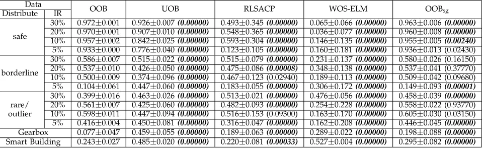
4.3 Comparison with Other Algorithms

This section compares MLP-based OOB and UOB with two state-of-the-art methods RLSACP and WOS-ELM. OOB with a single MLP is included as a benchmark, denoted by OOBsg. Tables 5 - 6 present

TABLE 5: The final-step minority-class recall and statistical test results from MLP-based OOB, OOBsg, UOB,

RLSACP and WOS-ELM.

Data

OOB UOB RLSACP WOS-ELM OOBsg

Distribute IR

safe

30% 0.973±0.004(0.00000) 0.986±0.001 0.490±0.344(0.00000) 0.332±0.466(0.00000) 0.959±0.016(0.00000)

20% 0.979±0.003(0.00000) 0.992±0.007 0.551±0.373(0.00000) 0.283±0.443(0.00000) 0.960±0.026(0.00000)

10% 0.923±0.005(0.00620) 0.900±0.048 0.593±0.302(0.00000) 0.586±0.466 (0.97450) 0.920±0.010 (0.0231)

5% 0.880±0.000(0.00000) 0.741±0.120 0.027±0.025(0.00000) 0.414±0.449 (0.02530) 0.884±0.025(0.00000)

borderline

30% 0.488±0.016(0.00000) 0.828±0.036 0.512±0.020(0.00000) 0.194±0.286(0.00000) 0.515±0.074(0.00000)

20% 0.369±0.017(0.00000) 0.854±0.055 0.535±0.028(0.00000) 0.520±0.341(0.00002) 0.392±0.079(0.00000)

10% 0.293±0.011(0.00000) 0.806±0.106 0.481±0.064(0.00000) 0.296±0.398(0.00000) 0.315±0.060(0.00000)

5% 0.015±0.008(0.00000) 0.456±0.212 0.039±0.017(0.00000) 0.417±0.348 (0.21640) 0.032±0.026(0.00000)

30% 0.196±0.019(0.00000) 0.727±0.047 0.493±0.115(0.00000) 0.559±0.149(0.00000) 0.303±0.072(0.00000)

rare/ 20% 0.370±0.011(0.00000) 0.853±0.052 0.468±0.015(0.00000) 0.234±0.266(0.00000) 0.391±0.040(0.00000)

outlier 10% 0.390±0.015(0.00000) 0.839±0.088 0.521±0.144(0.00000) 0.363±0.419(0.00000) 0.408±0.044(0.00000)

5% 0.181±0.004(0.00000) 0.479±0.200 0.111±0.030(0.00000) 0.164±0.270(0.00000) 0.212±0.045(0.00000)

Gearbox 0.008±0.005(0.00000) 0.697±0.110 0.042±0.023(0.00000) 0.888±0.022(0.00000) 0.049±0.037(0.00000)

Smart Building 0.065±0.014(0.00000) 0.552±0.075 0.161±0.280(0.00000) 0.484±0.011(0.00000) 0.109±0.058(0.00000)

TABLE 6: The final-step G-meanand statistical test results from MLP-based OOB, OOBsg, UOB, RLSACP and

WOS-ELM.

Data

OOB UOB RLSACP WOS-ELM OOBsg

Distribute IR

safe

30% 0.972±0.001 0.926±0.007(0.00000) 0.493±0.345(0.00000) 0.065±0.066(0.00000) 0.963±0.006(0.00000)

20% 0.970±0.001 0.907±0.010(0.00000) 0.548±0.365(0.00000) 0.036±0.077(0.00000) 0.960±0.008(0.00000)

10% 0.957±0.002 0.842±0.025(0.00000) 0.593±0.304(0.00000) 0.146±0.135(0.00000) 0.955±0.005(0.00240)

5% 0.933±0.000 0.776±0.040(0.00000) 0.123±0.105(0.00000) 0.160±0.181(0.00000) 0.936±0.013 (0.02430)

borderline

30% 0.586±0.007 0.515±0.022(0.00000) 0.515±0.079(0.00000) 0.231±0.137(0.00000) 0.580±0.026 (0.16150)

20% 0.537±0.010 0.426±0.050(0.00000) 0.475±0.086(0.00008) 0.348±0.138(0.00000) 0.537±0.041 (0.37770)

10% 0.500±0.009 0.374±0.096(0.00000) 0.467±0.123 (0.02940) 0.189±0.113(0.00000) 0.509±0.042 (0.09680)

5% 0.104±0.061 0.447±0.060(0.00000) 0.183±0.055(0.00000) 0.306±0.172(0.00000) 0.149±0.093(0.00001)

30% 0.399±0.016 0.463±0.026(0.00000) 0.513±0.021(0.00000) 0.476±0.056(0.00000) 0.458±0.039(0.00000)

rare/ 20% 0.561±0.007 0.425±0.060(0.00000) 0.482±0.093(0.00000) 0.254±0.228(0.00000) 0.558±0.022 (0.93770)

outlier 10% 0.598±0.011 0.447±0.094(0.00000) 0.516±0.153 (0.09300) 0.163±0.170(0.00000) 0.605±0.030 (0.03150)

5% 0.416±0.004 0.450±0.081(0.00000) 0.316±0.047(0.00000) 0.162±0.208(0.00000) 0.446±0.045(0.00000)

Gearbox 0.077±0.047 0.459±0.055(0.00000) 0.189±0.063(0.00000) 0.289±0.022(0.00000) 0.198±0.088(0.00000)

Smart Building 0.243±0.027 0.485±0.020(0.00000) 0.220±0.081(0.00033) 0.527±0.004(0.00000) 0.295±0.082(0.00000)

the winner of G-mean. The Wilcoxon Sign Rank test is thus carried out between UOB and every other method for minority-class recall and between OOB and every other method for G-mean. There are 56 pairs of comparison for each metric. P-values are included in the tables.

Although undersampling in MLP-based UOB im-proves minority-class recall greatly, we notice that the majority-class recall is dragged down too much, which explains why its overall performance is worse than OOB. RLSACP and WOS-ELM outperform OOB in terms of minority-class recall in some cases. How-ever, because their majority-class recall is decreased more than the increase of minority-class recall, their G-mean does not beat OOB’s. Besides, we notice that WOS-ELM presents very large performance vari-ance in many cases. This is caused by the fact that the minority-class examples are overemphasized and the majority-class performance is sacrificed greatly in some runs. A possible explanation for this phe-nomenon is that the extreme learning machine (ELM) used in WOS-ELM was found to be sensitive to outliers in data and lacks robustness sometimes [32]. Especially after the minority class is further empha-sized by a higher weight in WOS- ELM, the empirical

risk minimization principle of ELM is more likely to lead to great bias towards the minority class.

OOB and OOBsg have similar performance. OOBsg

shows better G-mean than RLSACP and WOS-ELM in most cases. This observation confirms that resampling is the main reason for OOB and UOB outperforming RLSACP and WOS-ELM, rather than the ensemble of classifiers.

Generally speaking, among these perceptron-based methods, UOB is the best at recognizing minority-class examples; OOB is the best at balancing the performance between classes. Comparing between tree-based OOB/UOB and MLP-based OOB/UOB, we conclude that the decision tree is preferable to MLP as the base learner of OOB and UOB, based on the observation that tree-based ensembles outperform MLP-based ensembles in most cases.

4.4 Factorial Analysis of Data-Related Factors and Base Classifiers

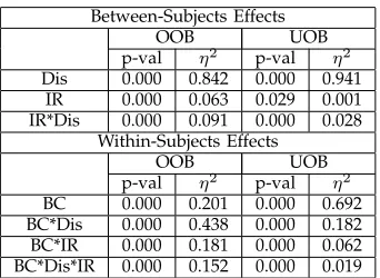
by types of class imbalance and base classifiers. Three factors are analysed: data distributions, IR and base classifiers. There are 3 different levels (settings) for ‘distribution’ (safe, borderline, rare/outlier) and 4 different levels for IR (5%, 10%, 20% and 30%). We consider 2 levels (types) of base classifiers – decision tree and MLP. A mixed design is necessary, because the distribution and IR are between-subjects factors (their levels vary with the data being used), and the base classifier is a within-subjects factor (its levels vary within the data). The factorial design allows the effects of a factor to be estimated at several levels of the other factors. The effects of the factors on the final-step G-mean is discussed. The metric under observation is also called “response” in the context of ANOVA.

The ANOVA results are presented in Table 7, including p-value and eta-squared (η2_{). A p-value} smaller than 0.05 indicates a significant difference by rejecting the null hypothesis under the significance level of 5%. η2 is a measure in the range of [0,1] describing the effect size. The larger theη2, the greater the effect of the factor. It is worth mentioning here that η2 is calculated separately for between-subjects and within-subjects factors [33]. For the cases with only between-subjects factors and the cases involving within-subjects factors, the sum of η2 _{of the factor} effects and the associated standard errors is equal to 1 respectively. Besides, the assumption of sphericity in ANOVA based on Mauchly’s test is not an issue here, because there are only two levels (i.e. one pair of data groups) for the within-subjects factor. Mauchly’s test examines whether the level of dependence between pairs of groups is equal.

TABLE 7: Factor effects of data distributions (abbr. Dis), imbalance rates (abbr. IR) and base classifiers (abbr. BC), and their interaction effects on G-mean from OOB and UOB. The symbol “*” indicates the interaction between two factors.

Between-Subjects Effects

OOB UOB

p-val η2 _{p-val η}2

Dis 0.000 0.842 0.000 0.941

IR 0.000 0.063 0.029 0.001

IR*Dis 0.000 0.091 0.000 0.028

Within-Subjects Effects

OOB UOB

p-val η2 _{p-val η}2

BC 0.000 0.201 0.000 0.692

BC*Dis 0.000 0.438 0.000 0.182

BC*IR 0.000 0.181 0.000 0.062

BC*Dis*IR 0.000 0.152 0.000 0.019

Table 7 shows the factor effects on G-mean. All the p-values are much smaller than 0.05, suggesting that all the three factors and their interactions have a significant impact on G-mean. According to η2, the effect of data distribution (0.842 for OOB and 0.941 for UOB) is much larger than the effects of

IR (0.063 for OOB and 0.001 for UOB) and the base classifier (0.201 for OOB and 0.692 for UOB). The effect of IR on UOB is much smaller than that on OOB, suggesting that UOB is less sensitive to the imbalance rate. The effect of base classifiers on OOB is much smaller than that on UOB, suggesting that OOB is less sensitive to the choice of base classifiers. Generally speaking, the minority-class distribution is a major factor affecting the performance of OOB and UOB, compared to which their performance is quite robust to the imbalance rate.

5

C

I

A

D

D

S

This section focuses on the dynamic feature of on-line class imbalance. Different from existing concept drift methods that mainly aim for changes in class-conditional probability density functions, we look into the performance of OOB and UOB when tackling data streams with imbalance status changes (i.e. changes in class prior probabilities). In other words, IR is chang-ing over time. It happens in real-world problems. For example, given the task of detecting faults in a running engineering system, the faulty class is usually the minority class that rarely occurs. The faults can become more and more frequent over time, if the damaged condition gets worse; or the faults are not likely to happen from some moment, because the faulty system is repaired. Dynamic data are more challenging than static ones, because the online model needs to sense the change and then adjust its learning bias quickly to maintain its performance. Different types of changes in imbalance status are designed and studied in this section, varying in changing speed and severity.

The adaptivity and robustness of OOB and UOB are studied by answering the following questions: 1) how does the time-decayed metric used in OOB and UOB help to handle the imbalance change? 2) How do OOB and UOB perform in comparison with other state-of-the-art algorithms under dynamic scenarios? 3) How is their performance affected by the decay factor? For the first question, OOB and UOB are compared with those applying the traditional method of updating the class size. For the second question, OOB and UOB are compared with RLSACP and WOS-ELM. For the final question, ANOVA using a repeated measure design is performed to analyse the impact of the decay factor.

5.1 Data Description and Experimental Settings

5.1.1 Data

Three data sources are used to produce dynamic data streams – Gaussian data, Gearbox and Smart Building. By using the same data generation method as de-scribed in Section 4.1, we produce two-class Gaussian data streams formed of two numeric attributes and a class label that can be +1 or -1. Each class follows the multivariate Gaussian distribution. Some overlapping between classes is enabled for a certain level of data complexity. Gearbox and Smart Building are fault de-tection data from the real-world applications used in the previous section, containing a faulty class (+1) and a nonfaulty class (-1). We limit the length of each data stream to 1000 examples. Different from static data streams, the dynamic ones involve a class imbalance change right after time step 500. During the first 500 time steps, IR is fixed to 10% and the positive class is the minority. From time step 501, a change occurs at a certain speed and severity. Four data streams are generated from each data source. Each type is a combination of two changing severity levels and two changing speeds. The changing severity can be either high or low; the changing speed can be either abrupt or gradual. The concrete change settings are:

• High severity: the negative class becomes the

minority with IR 10% in the new status.

• _{Low severity: the data stream becomes balanced}

(i.e. IR = 50%) in the new status.

• Abrupt change: the length of the changing period

is 0. The new status completely takes over the data stream from time step 501.

• Gradual change: the change lasts for 300 time

steps. During the changing period, the probabil-ity of examples being drawn from the old joint distribution decreases linearly.

5.1.2 Settings

When studying how the time-decayed class size w(_kt)

in OOB and UOB helps the classification in dynamic data streams, we replace w(_kt) with the class size updated in the traditional way, which considers all observed examples so far equally. For example, if 50 majority-class examples and 10 minority-class exam-ples have been observed so far, then the oversampling rate for OOB is set to 5 and the undersampling rate for UOB is set to 0.2 at the current moment. We use OOBtrand UOBtrto stand for OOB and UOB using the

traditional size update in the following analysis. All the methods here build an ensemble model composed of 50 Hoeffding trees.

When discussing the adaptivity of OOB and UOB in comparison with RLSACP and WOS-ELM, MLP is used as the base classifier of OOB and UOB as before. Both OOB and UOB consist of 50 MLPs. OOB with a single MLP (OOBsg) is included as the benchmark.

The window size for updating the error cost of classes is shortened to 50 time steps in RLSACP, to encourage

a faster response to the change. The error cost in the original WOS-ELM was updated based on a separate validation data set in the original article [22], which however may not be available in many real-world problems, or expire over time. To allow the same level of adaptivity as OOB and UOB, the time-decayed class sizes are used to set the costs in WOS-ELM. Specifically, the error cost of the majority class is always equal to 1; the error cost of the minority class is set tow_maj(t) /w(_mint) , wherew(_majt) andw(_mint) are the time-decayed sizes of the current majority and minority classes respectively.

The same as in Section 4, the prequential recall and G-mean are tracked to observe the performance before and after the change. For a clear and accurate understanding of OOB and UOB learning dynamic data, we divide the prequential evaluation process into three stages, old-status stage, changing stage and new-status stage, by resetting the performance metrics to 0 between the stages. In more details, for the data with an abrupt change (where there is no changing stage), recall and G-mean are reset after time step 500, when the change starts and ends; for the data with a gradual change (where the changing stage is 300 time-step long), recall and G-mean are reset after time step 500 and 800. This is to ensure that the performance observed after the change is not affected by the performance before the change. Prequential performance curves will be presented to help visualize the performance behaviors at each time step and the impacts of changes. For a quantitative understanding, we will provide the average prequen-tial performance covering all the time steps during the new-status stage. It can better reflect the influence of the status change than the final-step performance. The Wilcoxon Sign Rank test with Holm-Bonferroni corrections is applied for statistical analysis.

5.2 Role of the Time-Decayed Metric

In this section, we aim to find out: 1) how different types of imbalance changes affect the performance of OOB and UOB; 2) whether and how the time-decayed class size in OOB and UOB facilitates learn-ing in dynamic data streams, through the comparison with OOBtr and UOBtr. To understand the impact of

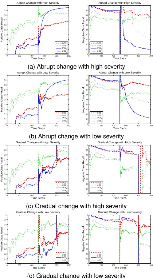
change on each class, we monitor the behaviours of prequential recall of minority and majority classes individually along with time.

Fig. 1 presents the recall curves produced from the data streams using data source Smart Building. For the abrupt change with high severity, before the change happens, UOB and UOBtr have better

minority(positive)-class recall than OOB and OOBtr,

a rapid growth in recall, especially for OOBtr and

UOBtr. The growth is caused by the frequent arrival

of positive-class examples; OOBtrand UOBtrincrease

faster than OOB and UOB, because the imbalance status obtained by using the traditional method still shows that this class is the minority within a period of time after the change. So, the wrong resampling technique is applied, which emphasizes this class even when it has become the majority. The time-decayed class size in OOB and UOB reflects the correct imbalance status quickly, and thus OOB and UOB adjust their focus on the correct class after the change.

0 200 400 600 800 1000

0 0.1 0.2 0.3 0.4 0.5 0.6 0.7 0.8 0.9 1 Time Steps

Positive Class Recall

Abrupt Change with High Severity

OOB UOB OOBtr UOBtr

0 200 400 600 800 1000

0 0.1 0.2 0.3 0.4 0.5 0.6 0.7 0.8 0.9 1 Time Steps

Negative Class Recall

Abrupt Change with High Severity

OOB UOB OOBtr UOBtr

(a) Abrupt change with high severity

0 200 400 600 800 1000

0 0.1 0.2 0.3 0.4 0.5 0.6 0.7 0.8 0.9 1 Time Steps

Positive Class Recall

Abrupt Change with Low Severity

OOB UOB OOBtr UOBtr

0 200 400 600 800 1000

0 0.1 0.2 0.3 0.4 0.5 0.6 0.7 0.8 0.9 1 Time Steps

Negative Class Recall

Abrupt Change with Low Severity

OOB UOB OOBtr UOBtr

(b) Abrupt change with low severity

0 200 400 600 800 1000

0 0.1 0.2 0.3 0.4 0.5 0.6 0.7 0.8 0.9 1 Time Steps

Positive Class Recall

Gradual Change with High Severity

OOB UOB OOBtr UOBtr

0 200 400 600 800 1000

0 0.1 0.2 0.3 0.4 0.5 0.6 0.7 0.8 0.9 1 Time Steps

Negative Class Recall

Gradual Change with High Severity

OOB UOB OOBtr UOBtr

(c) Gradual change with high severity

0 200 400 600 800 1000

0 0.1 0.2 0.3 0.4 0.5 0.6 0.7 0.8 0.9 1 Time Steps

Positive Class Recall

Gradual Change with Low Severity

OOB UOB OOBtr UOBtr

0 200 400 600 800 1000

0 0.1 0.2 0.3 0.4 0.5 0.6 0.7 0.8 0.9 1 Time Steps

Negative Class Recall

Gradual Change with Low Severity

OOB UOB OOBtr UOBtr

(d) Gradual change with low severity

Fig. 1: Prequential recall curves of positive (left) and negative (right) classes from OOB, UOB, OOBtr and

UOBtron Smart Building data with 4 types of changes.

In terms of negative-class recall, when this class turns from the majority to the minority, all the

meth-ods present a more or less reduced recall; OOB is the most resistant. One reason for the reduction is the performance trade-off between classes. As the positive class becomes the majority with a great per-formance improvement, the perper-formance of the other class would be compromised to some extent. UOB suffers from a greater reduction than OOB right after the change, because undersampling makes the online model learn less knowledge about this class before the change. Even so, the recall from UOB recovers faster than OOBtr and UOBtr. When OOBtr and UOBtr still

treat this class as the majority after the change, UOB has already realized its minority status and applied undersampling to the other class. The robustness of OOB and the adaptivity of UOB prove the benefits of using time-decayed class size and the importance of considering real-time status of data streams.

The other three types of changes present similar results. The positive-class recall presents a fast in-crease, and the negative-class recall is decreased, after the change occurs. Among the four methods, UOB is the best at recognizing the minority-class examples before the change; OOB is the most resistant method to changes; UOB is affected more by the changes than OOB on the old majority class, but its performance recovers faster than OOBtr and UOBtr. For the space

consideration, the plots from Gaussian and Gearbox were omitted, from which similar results are obtained. To understand how the overall performance is af-fected, we compare average G-mean over the new-status stage. Table 8 shows its means and standard deviations from 100 runs for the Smart Building data. P-values from the Wilcoxon Sign Rank test between OOB and every other method are included in brack-ets, among which the ones in bold italics suggest a significant difference. We can see that OOBtr and

UOBtr are significantly worse than OOB and UOB,

because of the incorrectly detected imbalance rate. Although the above results show that UOB suffers from a performance reduction on the old majority class, its G-mean still outperforms OOB in some cases, because of its fast performance recovery on this class through undersampling using the correctly estimated imbalance rate.

In conclusion, when there is an imbalance status change in the data stream, OOB is the least affected. A performance drop on the old majority class occurs to UOB after the change, but its performance recovers rapidly. It is necessary to use the time-decayed metric for choosing the correct resampling technique and estimating the imbalance status.

5.3 Comparison with Other Algorithms

TABLE 8:Average G-meanduring the new-status stage and statistical test results from tree-based OOB, UOB, OOBtrand UOBtr on Smart Building. (Change type: H, high severity; L, low severity; A, abrupt; G, gradual)

Change OOB UOB OOBtr UOBtr

H A 0.693±0.004 0.763±0.012(0.00000) 0.389±0.018(0.00000) 0.662±0.016(0.00000)

H G 0.609±0.001 0.462±0.012(0.00000) 0.000±0.000(0.00000) 0.208±0.123(0.00000)

L A 0.675±0.002 0.701±0.006(0.00000) 0.446±0.025(0.00000) 0.639±0.006(0.00000)

L G 0.679±0.001 0.683±0.020 (0.29420) 0.000±0.000(0.00000) 0.511±0.022(0.00000)

TABLE 9:Average G-meanduring the new-status stage and statistical test results from MLP-based OOB, OOBsg,

UOB, RLSACP and WOS-ELM. (Change type: H, high severity; L, low severity; A, abrupt; G, gradual)

Data Change OOB UOB RLSACP WOS-ELM OOBsg

Gaussian

H A 0.532±0.034 0.019±0.013(0.00000) 0.366±0.096(0.00000) 0.090±0.125(0.00000) 0.544±0.049 (0.07080)

H G 0.360±0.002 0.359±0.011(0.00440) 0.388±0.089 (0.04490) 0.037±0.095(0.00000) 0.350±0.010(0.00000)

L A 0.795±0.003 0.521±0.025(0.00000) 0.439±0.210(0.00000) 0.022±0.074(0.00000) 0.778±0.013(0.00000)

L G 0.811±0.001 0.758±0.015(0.00000) 0.613±0.118(0.00000) 0.015±0.056(0.00000) 0.813±0.010(0.00160)

Gearbox

H A 0.293±0.009 0.201±0.032(0.00000) 0.438±0.012(0.00000) 0.000±0.000(0.00000) 0.261±0.113 (0.54110)

H G 0.000±0.000 0.364±0.119(0.00000) 0.140±0.126(0.00000) 0.000±0.000 (NaN) 0.161±0.177(0.00000)

L A 0.452±0.014 0.479±0.012(0.00000) 0.378±0.031(0.00000) 0.000±0.000(0.00000) 0.430±0.056 (0.01470)

L G 0.408±0.032 0.432±0.023(0.00000) 0.055±0.095(0.00000) 0.000±0.000(0.00000) 0.373±0.080(0.00078)

H A 0.276±0.028 0.261±0.052 (0.04740) 0.135±0.156(0.00000) 0.123±0.008(0.00000) 0.229±0.131 (0.03530)

Smart H G 0.000±0.000 0.140±0.091 (0.12090) 0.157±0.188(0.00000) 0.000±0.000 (NaN) 0.063±0.094(0.00000)

Building L A 0.451±0.019 0.435±0.016(0.00000) 0.228±0.144(0.00000) 0.000±0.000(0.00000) 0.441±0.044 (0.23750)

L G 0.443±0.023 0.485±0.018(0.00000) 0.080±0.078(0.00000) 0.000±0.000(0.00000) 0.374±0.112(0.00000)

Average G-mean over the new-status stage and the p-values produced from the Wilcoxon Sign Rank test between OOB and the others are shown in Table 9. “NaN” p-value in the table means that the two groups of samples for the statistical test are exactly the same. The results show that MLP-based OOB and UOB are quite competitive. In Gaussian data, UOB shows worse G-mean than OOB, because the imbalance change causes larger recall degradation on the old ma-jority class. In Gearbox and Smart Building data, OOB produces zero G-mean in 2 cases, which is caused by zero negative-class recall. In these two cases where the negative class turns from the majority to the minority gradually, because OOB is not so aggressive as UOB at recognizing minority-class examples, it could not adjust the learning bias to the new minority class quickly enough. That is not observed in tree-based OOB, as the decision tree was shown to be a more stable base classifier than MLP based on the results in Section 4. OOB and UOB outperform RLSACP and WOS-ELM in most cases. Although WOS-ELM applies the same time-decayed metric for updating misclassification costs as in OOB and UOB, its G-mean remains zero in many cases, caused by the zero recall of the old minority class. This class is not well learnt before the change, and its recall value remains low after the change because no emphasis is given to this class. Resampling is simply a better class imbalance strategy than adjusting class costs through the comparison with OOBsg, which tallies with our

observation in the previous section.

5.4 Factorial Analysis of the Decay Factor

Section 5.2 has shown the key role of using the time-decayed class size w_k(t) for deciding the resampling rate in OOB and UOB. According to our preliminary

experiments [6], the decay factor θ in its definition formula (Eq. 1) is set to 0.9 in the above experi-ments. Too small values of θ (< 0.8) emphasize the current performance too much, which can affect the performance stability considerably. On the contrary, too large values (>0.95) can deteriorate the adaptivity of online models to dynamic changes. Within a rea-sonable setting range, this section studies the impact of the decay factor on the performance of OOB and UOB statistically. One-way ANOVA using a repeated measure design is conducted.

We choose three levels (settings) for the factorθ – 0.8, 0.9 and 0.95. DT-based OOB and UOB are applied to the Smart Building data with an abrupt change in high severity, under each setting of θ. The response in this ANOVA is the average prequential G-mean during the new-status stage of class imbalance. It is worth nothing that the data groups under different factor levels violate the assumption of sphericity in ANOVA based on Mauchly’s test, i.e. the level of dependence between pairs of groups is not equal. Therefore, Greenhouse-Geisser correction is used [34]. The ANOVA and performance results are shown in Table 10.

TABLE 10: ANOVA results and average G-mean from OOB and UOB after the change.

ANOVA Average G-mean

p-val η2 _{θ= 0.8 θ= 0.9 θ= 0.95}

OOB 0.000 0.989 0.726 0.693 0.643

UOB 0.018 0.077 0.763 0.763 0.760

performance, implying that adapting to the change sooner may help OOB to respond to the new minority class better. UOB is less sensitive to the setting ofθ.

6

E

OOB

UOB

UOB has been shown to be a better choice than OOB in terms of minority-class recall and G-mean. However, it has some weaknesses when the majority class in the data stream turns into the minority class. OOB has been shown to be more robust against changes. To combine the strength of OOB and UOB, this section proposes new methods based on the idea of ensembles, which train and maintain both OOB and UOB. A weight is maintained for each of them, adjusted adaptively according to their current performance measured by G-mean. Their combined weighted vote will decide the final prediction.

Recalling the definition of time-decayed recall R(t) in Section 2.1, we use R(t) _{to calculate real-time} G-mean for deciding the weights of online learners. It is adaptive to dynamic changes through the time decay factor, and reflects the current performance better than the prequential recall. However, we find that

R(t) presents a large variance between time steps, which may result in misleading and unstable weights. So, we introduce the simple moving average (SMA) technique to smooth out the short-term fluctuations ofR(t)_{curves. Givenl values ofR}(t)_{, smoothed recall}

SR(t)_{at time stept is defined as,}

SR(t)=R

(t)_{+. . .+R}(t−bl/2c)_{+. . .+R}(t−l)

l .

SR(t)looks back l time steps for the smoother recall. Using SR(t)_{, we next introduce the weighted} ensem-ble methods of OOB and UOB, tested on the real-world data in comparison with individual OOB and UOB.

6.1 Weighted Ensemble of OOB and UOB

By calculating SMA of recall of both classes, we can obtain current G-mean. It is used to determine the weights of OOB and UOB. Their weighted ensemble, denoted as WEOB, is expected to be both accurate and robust in dynamic environments, as it adopts the better strategy (OOB or UOB) for different situations. Two weight adjusting strategies are proposed and compared here. Suppose OOB has G-mean value go and UOB has G-mean valueguat the current moment. Let αo and αu denote the weights of OOB and UOB respectively. In the first strategy, normalized G-mean values of OOB and UOB are used as their weights:

αo=

go

go+gu

, αu=

gu

go+gu

.

In the second strategy, the weights can only be binary values (0 or 1):

(

αo= 1, αu= 0 if go≥gu

αo= 0, αu= 1 if go< gu

In other words, the final prediction will solely depend on the online model with the higher G-mean. Let’s denote these two strategies as WEOB1 and WEOB2. WEOB1 follows the traditional idea of ensemble. From the statistical point of view, combining the outputs of several classifiers by averaging can reduce the risk of an unfortunate selection of a poorly performing classifiers and thus provide stable and accurate per-formance [35], although the averaging may or may not beat the performance of the best classifiers in the ensemble (used by WEOB2). Therefore, it is worth looking into both strategies.

6.2 Data Description and Experimental Settings

To compare WEOB1 and WEOB2 with OOB and UOB, we generate two data streams from real-world appli-cations Gearbox and Smart Building. Each data stream contains 5000 time steps. At every 500 time steps, our data generation algorithm randomly chooses one class to be the minority class, and fixes the imbalance rate randomly chosen from set {5%, 10%, 20%}. By doing so, there could be an abrupt change in the class imbalance status after every 500 examples have arrived. The detailed information of the resulting data is summarized in Table 11, including which class belongs to the minority during which period of time.

TABLE 11: Data Stream Description.

Data Class label Time steps of being minority

Gearbox Positive 1-500, 1501-2000, 3001-4500

Negative 501-1500, 2001-3000, 4501-5000

Smart Building Positive 1-500, 1501-2000, 3001-4000

Negative 501-1500, 2001-3000, 4001-5000

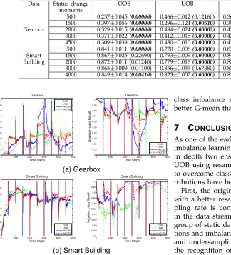
WEOB1 and WEOB2 combine one OOB and one UOB composed of 50 base classifiers respectively. All methods use Hoeffding tree as the base classifier.l is set to 51 for calculatingSR(t). All the other parameter settings remain the same. Prequential recall and G-mean are recorded at each time step. The performance metrics are reset to 0 after every 500 time steps for a clear observation.

6.3 Experimental Analysis

TABLE 12: Average G-meanfrom tree-based OOB, UOB, WEOB1 and WEOB2 during the 500 time steps after each status change, and statistical test results (in brackets). Values in bold italics indicate a statistically significant difference.

Data Status change OOB UOB WEOB1 WEOB2

moments

Gearbox

500 0.237±0.045(0.00000) 0.466±0.012 (0.12160) 0.364±0.014(0.00000) 0.463±0.012

1500 0.397±0.056(0.00000) 0.296±0.124(0.00510) 0.395±0.079 (0.00830) 0.404±0.072

2000 0.329±0.015(0.00000) 0.494±0.024(0.00002) 0.424±0.018(0.00000) 0.485±0.024

3000 0.371±0.022(0.00000) 0.412±0.015(0.00000) 0.437±0.015(0.00000) 0.458±0.025

4500 0.309±0.039(0.00000) 0.480±0.010(0.00000) 0.424±0.023(0.00000) 0.443±0.024

500 0.841±0.011(0.00000) 0.770±0.008(0.00000) 0.821±0.016(0.00200) 0.831±0.015

Smart 1500 0.867±0.025 (0.22690) 0.793±0.009(0.00000) 0.843±0.011(0.00000) 0.865±0.022

Building 2000 0.872±0.011 (0.01240) 0.779±0.016(0.00000) 0.886±0.003(0.00000) 0.868±0.015

3000 0.865±0.009 (0.04100) 0.856±0.035 (0.67880) 0.854±0.002 (0.18780) 0.861±0.013

4000 0.849±0.014(0.00410) 0.823±0.007(0.00000) 0.839±0.005 (0.17010) 0.842±0.017

0 1000 2000 3000 4000 5000 0

0.1 0.2 0.3 0.4 0.5 0.6 0.7 0.8 0.9 1

Time Steps

Positive−class Recall

Gearbox

OOB UOB WEOB1 WEOB2

0 1000 2000 3000 4000 5000 0

0.1 0.2 0.3 0.4 0.5 0.6 0.7 0.8 0.9 1

Time Steps

Negative−class Recall

Gearbox

OOB UOB WEOB1 WEOB2

(a) Gearbox

0 1000 2000 3000 4000 5000 0.2

0.3 0.4 0.5 0.6 0.7 0.8 0.9 1

Time Steps

Positive−class Recall

Smart Building

OOB UOB WEOB1 WEOB2

0 1000 2000 3000 4000 5000 0.5

0.55 0.6 0.65 0.7 0.75 0.8 0.85 0.9 0.95 1

Time Steps

Negative−class Recall

Smart Building

OOB UOB WEOB1 WEOB2

(b) Smart Building

Fig. 2: Prequential recall of positive (left) and negative (right) classes.

With respect to the overall performance, Table 12 compares the average prequential G-mean during the 500 time steps after each status change, including its mean and standard deviation over 100 runs, and the p-values from Wilcoxon Sign Rank test performed between WEOB2 and every other method. The com-parative results from this table tally with our results on recall. WEOB1 and WEOB2 are better than or locate in between single OOB and UOB in 9 out of 10 cases. On the Gearbox data, WEOB2 is competitive with UOB, and outperforms the other two in most cases significantly; on the Smart Building data, WEOB2 seems to be slightly worse than OOB, and better than the other two in most cases. Overall, WEOB2 outperforms WEOB1 significantly in 6 out of 10 cases, in terms of G-mean.

Generally speaking, WEOB1 and WEOB2 success-fully combine the strength of OOB and UOB. They achieve high performance in terms of recall and G-mean, and show good robustness to changes in the

class imbalance status. Particularly, WEOB2 shows better G-mean than WEOB1.

7

C

As one of the earliest works focusing on online class imbalance learning, this paper improved and studied in depth two ensemble learning methods OOB and UOB using resampling and the time-decayed metric to overcome class imbalance online. Four major con-tributions have been made.

UOB. WEOB2 outperformed WEOB1 in terms of G-mean.

In the future, we would like to extend our work to multi-class cases. Second, we would like to study our methods in data streams with concept drifts. Third, the work presented in this paper relied heavily on computational experiments. More theoretical studies will be given.

A

This work was supported by two European Com-mission FP7 Grants (Nos. 270428 and 257906) and an EPSRC Grant (No. EP/J017515/1). Xin Yao was supported by a Royal Society Wolfson Research Merit Award.

R

[1] L. L. Minku, “Online ensemble learning in the presence of

concept drift,” Ph.D. dissertation, School of Computer Science, The University of Birmingham, 2010.

[2] H. He and E. A. Garcia, “Learning from imbalanced data,”

IEEE Transactions on Knowledge and Data Engineering, vol. 21, no. 9, pp. 1263–1284, 2009.

[3] N. C. Oza and S. Russell, “Experimental comparisons of online

and batch versions of bagging and boosting,” inProceedings of

the seventh ACM SIGKDD international conference on Knowledge discovery and data mining. ACM, 2001, pp. 359–364.

[4] J. Meseguer, V. Puig, and T. Escobet, “Fault diagnosis using

a timed discrete-event approach based on interval observers:

Application to sewer networks,”IEEE Transactions on Systems,

Man and Cybernetics, Part A: Systems and Humans, vol. 40, no. 5, pp. 900–916, 2010.

[5] G. M. Weiss, “Mining with rarity: a unifying framework,”

ACM SIGKDD Explorations Newsletter, vol. 6, no. 1, pp. 7–19, 2004.

[6] S. Wang, L. L. Minku, and X. Yao, “A learning framework

for online class imbalance learning,” in IEEE Symposium on

Computational Intelligence and Ensemble Learning (CIEL), 2013, pp. 36–45.

[7] N. C. Oza, “Online bagging and boosting,”IEEE International

Conference on Systems, Man and Cybernetics, pp. 2340–2345, 2005.

[8] N. Japkowicz and S. Stephen, “The class imbalance problem:

A systematic study,”Intelligent Data Analysis, vol. 6, no. 5, pp.

429 – 449, 2002.

[9] U. Bhowan, M. Johnston, M. Zhang, and X. Yao, “Evolving

diverse ensembles using genetic programming for

classifica-tion with unbalanced data,”IEEE Transactions on Evolutionary

Computation, vol. 17, no. 3, pp. 368–386, 2013.

[10] R. C. Prati, G. E. Batista, and M. C. Monard, “Class imbalances versus class overlapping: An analysis of a learning system

behavior,”Lecture Notes in Computer Science, vol. 2972, pp. 312–

321, 2004.

[11] V. Garcia, J. Sanchez, and R. Mollineda, “An empirical study of the behavior of classifiers on imbalanced and overlapped

data sets,”Progress in Pattern Recognition, Image Analysis and

Applications, vol. 4756, pp. 397–406, 2007.

[12] T. Jo and N. Japkowicz, “Class imbalances versus small

dis-juncts,” inACM SIGKDD Explorations Newsletter, vol. 6, 2004,

pp. 40–49.

[13] J. V. Hulse, T. M. Khoshgoftaar, and A. Napolitano, “Ex-perimental perspectives on learning from imbalanced data,” in Proceedings of the 24th international conference on Machine learning, 2007, pp. 935–942.

[14] C. Elkan, “The foundations of cost-sensitive learning,” in

Proceedings of the Seventeenth International Joint Conference on Artificial Intelligence (IJCAI’01), 2001, pp. 973–978.

[15] L. Breiman, “Bagging predictors,”Machine Learning, vol. 24,

no. 2, pp. 123–140, 1996.

[16] S. Chen, H. He, K. Li, and S. Desai, “MuSeRA: Multiple se-lectively recursive approach towards imbalanced stream data

mining,” inInternational Joint Conference on Neural Networks,

2010, pp. 1–8.

[17] S. Chen and H. He, “Towards incremental learning of non-stationary imbalanced data stream: a multiple selectively

re-cursive approach,”Evolving Systems, vol. 2, no. 1, pp. 35–50,

2010.

[18] G. Ditzler and R. Polikar, “Incremental learning of concept

drift from streaming imbalanced data,” IEEE Transactions on

Knowledge and Data Engineering, vol. 25, no. 10, pp. 2283 – 2301, 2013.

[19] H. M. Nguyen, E. W. Cooper, and K. Kamei, “Online learning

from imbalanced data streams,” inInternational Conference of

Soft Computing and Pattern Recognition (SoCPaR), 2011, pp. 347– 352.

[20] L. L. Minku and X. Yao, “DDD: A new ensemble approach for

dealing with concept drift,”IEEE Transactions on Knowledge and

Data Engineering, vol. 24, no. 4, pp. 619 –633, 2012.

[21] A. Ghazikhani, R. Monsefi, and H. S. Yazdi, “Recursive least square perceptron model for non-stationary and imbalanced

data stream classification,”Evolving Systems, vol. 4, no. 2, pp.

119–131, 2013.

[22] B. Mirza, Z. Lin, and K.-A. Toh, “Weighted online sequential

extreme learning machine for class imbalance learning,”

Neu-ral Processing Letters, vol. 38, no. 3, pp. 465–486, 2013.

[23] D. C. Montgomery,Design and Analysis of Experiments. Great

Britain: John Wiley and Sons, 2004.

[24] K. Napierala and J. Stefanowski, “Identification of different

types of minority class examples in imbalanced data,”Hybrid

Artificial Intelligent Systems, vol. 7209, pp. 139–150, 2012. [25] “2009 PHM challenge competition data set,” The Prognostics

and Health Management Society (PHM Society). [Online]. Available: http://www.phmsociety.org/references/datasets [26] M. P. Michaelides, V. Reppa, C. Panayiotou, and M.

Polycar-pou, “Contaminant event monitoring in intelligent buildings

using a multi-zone formulation,” in 8th IFAC Symposium on

Fault Detection, Supervision and Safety of Technical Processes (SAFEPROCESS), vol. 8, 2012, pp. 492–497.

[27] G. Hulten, L. Spencer, and P. Domingos, “Mining

time-changing data streams,” in Proceedings of the Seventh ACM

SIGKDD International Conference on Knowledge Discovery and Data Mining, 2001, pp. 97–106.

[28] MOA Massive online analysis: Real time analytics for data streams. [Online]. Available: http://moa.cms.waikato.ac.nz/ [29] S. Wang, L. L. Minku, D. Ghezzi, D. Caltabiano, P. Tino, and

X. Yao, “Concept drift detection for online class imbalance

learning,” inInternational Joint Conference on Neural Networks

(IJCNN ’13), 2013, pp. 1–8.

[30] S. Wang, L. L. Minku, and X. Yao, “Online class imbalance

learning and its applications in fault detection,”International

Journal of Computational Intelligence and Applications, vol. 12, pp. 1 340 001(1–19), 2013.

[31] M. Kubat and S. Matwin, “Addressing the curse of imbalanced

training sets: One-sided selection,” inProc. 14th International

Conference on Machine Learning, 1997, pp. 179–186.

[32] S. Ding, H. Zhao, Y. Zhang, X. Xu, and R. Nie, “Extreme

learning machine: algorithm, theory and applications,”

Arti-ficial Intelligence Review, p. (In Print), 2013.

[33] C. A. Pierce, R. A. Block, and H. Aguinis, “Cautionary note on reporting eta-squared values from multifactor anova designs,”

Educational and Psychological Measurement, vol. 64, pp. 916–924, 2004.

[34] S. W. Greenhouse and S. Geisser, “On methods in the analysis

of profile data,”Psychometrika, vol. 24, no. 2, pp. 95–112, 1959.

[35] R. Polikar, “Ensemble based systems in decision making,”