TEMPORAL AND PARAMETRIC STUDY OF TRAVELLER PREFERENCE HETEROGENEITY USING RANDOM PARAMETER LOGIT MODEL

TEMPORAL AND PARAMETRIC STUDY OF TRAVELLER

PREFERENCE HETEROGENEITY USING RANDOM PARAMETER

LOGIT MODEL

AHM Mehbub Anwar1_{, Kiet Tieu}2_{, Peter Gibson}3_{, Matthew J. Berryman}4_{, Khin Than}

Win5_{, Andrew McCusker}6_{, Pascal Perez}7

1, 4, 6, 7 _{SMART Infrastructure Facility, University of Wollongong, Wollongong NSW 2522, Australia} 2, 3, 5 _{Faculty of Engineering and Information Sciences, University of Wollongong, Wollongong NSW 2522,}

Australia

Received 4 August 2014; accepted 25 September 2014

Abstract: In travel demand models, traditional objective attributes (TOAs) are very commonly used as explanatory variables. Nowadays, it is understood that latent variables (LVs) also significantly influence travellers’ behaviour. A hybrid choice modelling approach allows LVs in mode choice utility functions to be addressed. Specifically, a hybrid random parameter logit (HRPL) model has been developed to explore these influences. In this study, a traditional RPL (TRPL) model is compared with an HRPL model. For the later model, a two-step approach (also known as sequential approach) is implemented to incorporate LVs in choice models. Step 1 is the estimation of a MIMIC (multiple indicators and multiple causes) model; a type of regression model with a latent dependent variable(s). Step 2 is the estimation of a choice model with random parameters; information from the first step is incorporated in the second step. The paper analyses and compares the results of applying these models to a real urban case study using two datasets: 2008/09 and 2010/11 household travel survey (HTS) of Sydney Statistical Division (SSD), and also evaluates the predicted changes of mode choice probabilities based on hypothetical scenarios. Our results show that the HRPL model is superior to TRPL models that ignore the effect of LVs on traveller choice. The minimal changes in the parameter coefficients between the two datasets for each model suggest that the changes in traveller choice behaviour are gradual. Three hypothetical scenarios are simulated to forecast the changes that would be relevant to transport policy responses.

Keywords: latent variables, traditional objective variables, modelling, comparison, forecasting, logit model, mode choice, policy.

1 _{Corresponding author: [email protected]}

1. Introduction and Past Studies

Changing urban structures and environments have motivated transport planners and policy makers to improve their understanding of traveller choices (Habib and Zaman, 2012).

equity of mobility is a desirable transport management outcome. A consumer-focused transport mode option is a major indicator of transportation well-being, which is also important for social well-being as a whole. Adequate and suitable modes of transport for diverse kinds of consumers reflect the efficiency of urban travel and transport system performance. Srinivasan and Walker (2009) observed that there are wide varieties of influences on sustainable travel behaviour and they are relevant to demographics, socioeconomics, and psychological factors.

The latent factors people consider in making their travel decisions are more salient than travel time and cost alone. Furthermore, people’s travel preferences are much more complex than their socio-economic and trip characteristics (Anwar et al., 2011). There is strong evidence in extant research that recent developments including latent variables, latent classes, structural equation modelling (SEM) and integrated frameworks have advanced ways to examine a wider array of variables that might inf luence travel behaviour. This framework explicitly considers psychological factors, such as attitudes and perceptions, using psychometric indicators instead of objective attribute (Johansson et al., 2006; Ben-Akiva et al., 1994; Gopinath, 1995; Walker and Ben-Akiva, 2002; Ashok et al., 2002; Temme et al., 2008).

It is argued that personal and alternative modal attributes alone are no longer sufficient to explain traveller choice (Anwar et al., 2011; Domarchi et al., 2008; Anwar et al., 2014; Anwar et al., 2013). It has been observed that many factors affecting urban mode choice behaviour are latent in nature (Habib and Zaman, 2012; Anwar et al., 2011 and 2013). For example, the effect of

transport mode on happiness and subjective well-being was investigated by Zeid (2009) who noticed that psychological variables influence utility function in traveller mode choice decision. Integrating LVs in mode choice models, therefore, helps to increase the explanatory power of the models to demonstrate traveller motivational behaviour (Anwar et al., 2011; Johansson et al., 2006; Anwar et al., 2014 and 2013). Such LVs are important factors in influencing mode choice. They are also difficult to capture within simple random utility maximisation (RUM)-based multinomial logit (MNL) or probit frameworks. For this reason, the hybrid nature discrete choice model has become more popular for investigating the nature of modal choice decision-making processes amongst many modes (Train, 2009).

In brief, this paper deals with how discrete mode choice models work using the example of an RPL model with six LVs and thirteen TOAs. In this study, two RPL models are developed: (i) traditional RPL (TRPL) in which only TOAs are included; and (ii) hybrid RPL (HRPL) in which LVs and TOAs are integrated concurrently. This study is implemented to model traveller preference heterogeneity and to make a comparison between two datasets in two different years. The paper proposes an approach for forecasting traveller mode choice behaviour considering hypothetical scenarios for policy intervention.

2. Data

The Sydney HTS is the largest and most comprehensive source of personal travel data, which is the key data source of this study. The HTS covers Sydney and Illawarra Statistical Divisions and the Newcastle Sub-Statistical Division. The investigation in this paper is confined to travel by residents of the Sydney Statistical Division (SSD) only. The HTS is the longest running household travel survey in Australia. It began in 1997 and has been operating continuously since then. The survey collects detailed trip information for each day of the year by face-to-face interview. This collection method ensured high data quality and maximised response rates too.

Socio-demographic information about the residents of the selected household are also collected. The respondents were requested to maintain a simple travel diary to record the details of all trips undertaken for their nominated 24-hour period. An interviewer then interviewed each respondent to collect the details of each trip. For further details about the HTS, please see BTS (2012).

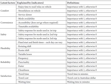
Six LVs and thirteen TOAs have been evaluated to model and compare the impact on travellers’ mode choice with predicted changes in mode choice probabilities. The selected LVs are: (i) comfort, (ii) convenience, (iii) safety, (iv) flexibility, (v) reliability, and (vi) satisfaction and twenty indicators described in Table 1 were set to explain them. The TOAs are: personal annual income (in Australian dollar), age (in years), gender (1 if male, 0 otherwise), having children (0-14 years), car ownership per adult, family size, full time workers of household, travel time (in minutes), travel cost (in Australian dollar), waiting time (in minutes), trip rate (trip per person per day), trip purpose (1 if work, 0 otherwise) and distance travelled (in kilometre).

Table 1

Description of Latent Variables

Latent factors Explained by (indicators) Definitions

Comfort

- Enjoy time to read/relax on vehicle Importance with 1, otherwise 0 - Stressfulness on vehicle Importance with 1, otherwise 0 - Service slower Importance with 1, otherwise 0

Convenience

- Mode availability Importance with 1, otherwise 0 - Accessibility (does not go where required) Importance with 1, otherwise 0 - Timetable availability Importance with 1, otherwise 0

Safety

- Safety response for mode used in 1st trip Importance with 1, otherwise 0 - Safety response for mode used in 2nd trip Importance with 1, otherwise 0 - Safety response for mode used in 3rd trip Importance with 1, otherwise 0

Flexibility

- Fixed start and finish times – each day can vary Importance with 1, otherwise 0 - Rotating shift Importance with 1, otherwise 0 - Roster shift Importance with 1, otherwise 0 - Variable hours Importance with 1, otherwise 0

Reliability

- Frequency Importance with 1, otherwise 0 - Punctuality Importance with 1, otherwise 0

- Faster Importance with 1, otherwise 0

Satisfaction

- Cleanliness Importance with 1, otherwise 0

- Travel time Travel time in minutes

- Travel cost Travel cost in Australian dollar - Waiting time Waiting time in minutes

For the empirical analysis with modelling and comparison, the 2008/09 and 2010/11 HTS data are used. For forecasting, only 2010/11 HTS data is used to be experienced about the policy responses. The selected variables and indicators from two datasets are same.

Reliability of the indicators listed in Table 1 was evaluated using factor analytic models (exploratory and confirmatory factor model) with the model fit criteria, such as GFI, AGFI, NFI, CFI and RMSEA with lower and upper bound. The factor analytic model focuses solely on how, and the extent to which, the observed variables are linked to their underlying latent factors (Byrne, 2010). Due to the limited space allocation for this paper, the results of measurement

equation (γ vector matrix of Eq. (2)) are not presented here. However, some results of them are available in Anwar et al. (2011).

3. Econometric Methods

We employ a similar econometric method that has been used in Anwar et al. (2014). However, there are two approaches available now for incorporating LVs into the choice

models (i) sequential approach, where the LVs

are needed to be constructed before being included into the discrete choice model as regular explanatory variables (Johansson et al., 2006; Ashok et al., 2002); and (ii)

more consistent and rational than other approach. Conversely, second approach is not popular due to its high complexity and the estimated results using both sequential and simultaneous approaches were not statistically different (Raveau et al., 2010) that motivated us to employ the first approach in this study.

3.1. Modelling with LVs

A M I M IC model, t hat def ines LVs appropriately, is estimated first, where the

LVs (η_ijl) are explained by characteristics (s_ijr)

from the users (individuals), alternatives (mode alternative) and trip nature through structural equation (Eq. (1)); as the analysts cannot collect data on LVs directly, indicators

(y_ijp) are assigned to explain them through

measurement equation (Eq. (2)):

ijl

r jlr ijr

ijl

α

s

ν

η

=

∑

∗

+

ijp ijl l jlp ijp

y

=

∑

γ

∗

η

+

ζ

where, i to an individual, j refers to an

alternative, l to a LV, r to an explanatory

variables belong to TOAs and p to an

indicator; α_jlr and γjlp are parameters to be

estimated, while ν_ijl and ζ_ijp are error terms

with mean zero and standard deviation to be estimated. The above specifications of MIMIC model are not restricted on the estimation of parameters and the results of model depend on the selected variables.

Specifications of Latent Variable Model

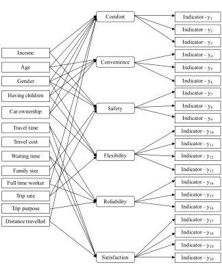
The factor analysis was employed to investigate the structural relationships in MIMIC model that guides the specification for computation of LVs (Fig. 1 illustrates the results of this process), which results in the following set of equations.

Comfortij = αinc-com,j*Incomei + αage-com,j*Agei + αgen-com,j*Genderi + αcar-com,j*Car ownershipi +

αftw-com,j*Full time workersi + dt-com,j*Distance travelled + αchi-com,j*Having children + νcom,ij

Convenienceij = αage-conv,j*Agei + αgen-conv,j*Genderi + αcar-conv,j*Car ownershipi + νconv,ij

Safetyij = αinc-saf,j*Incomei + αage-saf,j*Agei + αgen-saf,j*Genderi + αfs-saf,j*Family sizei + αtr-saf,j*Trip

ratei +νsaf,ij

Flexibilityij = αgen-fle,j*Genderi + αchi-fle,j*Having childreni + αcar-fle,j*Car ownershipi +

αtr-fle,j*Trip ratei + fle,ij

Reliabilityij = αtti-rel,j*Travel timei + αwti-rel,j*Waiting timei + αft-rel,j*Full time workersi +

αtp-rel,j*Trip purpopsei + rel,ij

Satisfactionij = αtti-sat,j*Travel timei + αtco-sat,j*Travel costi + αwti-sat,j*Waiting timei +

y_y1,ij = γ_y1,j * Comfort_ij + ζ_y1,ij y_y11,ij = γ_y11,j * Flexibility_ij + ζ_y11,ij

yy2,ij = γy2,j * Comfortij + ζy2,ij yy12,ij = γy12,j * Flexibilityij + ζy12,ij

yy3,ij = γy3,j * Comfortij + ζy3,iq yy13,ij = γy13,j * Flexibilityij + ζy13,ij

y_y4,ij = γ_y4,j * Convenience_ij + ζ_y4,ij y_y14,ij = γ_y14,j * Reliability_ij + ζ_y14,ij

yy5,ij = γy5,j * Convenienceij + ζy5,ij yy15,ij = γy15,j * Reliabilityij + ζy15,ij

y_y6,ij = γ_y6,j * Convenience_ij + ζ_y6,ij y_y16,ij = γ_y16,j * Reliability_ij + ζ_y16,ij

yy7ij = γy7,j * Safetyij + ζy7,ij yy17,ij = γy17,j * Satisfactionij + ζy17,ij

yy8,iq = γy8,j * Safetyij + ζy8,ij yy18,ij = γy18,j * Satisfactionij + ζy18,ij

y_y9,ij = γ_y9,j * Safety_ij + ζ_y9,ij y_y19,ij = γ_y19,j * Satisfaction_ij + ζ_y19,ij

yy10,ij = γy10,j * Flexibilityij + ζy10,ij yy20,ij = γy20,j * Satisfactionij + ζy20,ij

Convenience Comfort

Safety

Flexibility

Reliability

Satisfaction Income

Age

Gender

Having children

Car ownership

Travel time

Travel cost

Waiting time

Indicator - y1

Indicator – y2

Indicator – y3

Indicator – y4

Indicator – y5

Indicator – y12 Indicator – y6

Indicator – y14 Indicator – y9

Indicator – y13 Indicator – y7

Indicator – y8

Indicator – y10

Indicator – y11

Indicator – y15

Indicator – y16

Indicator – y17

Indicator – y18

Indicator – y19

Indicator – y20 Family size

Full time worker

Trip rate

Trip purpose

Distance travelled

Fig. 1.

3.2. Hybrid Discrete Choice Modelling

By maximising the utility (U_ij), individuals

take a decision based on the assumption of random utility theory. It is also assumed that an analyst can only determine a representative portion (systematic

component) of utility (V_ij) function,

therefore, an error term (εij) to each

alternative (Ortuzar and Willumsen, 2001) is required to be included in the function as stochastic component. Mathematically the utility function becomes as below (Eq. (3)):

U_ij = V_ij + εij, (3)

where Vij is a function of objective attributes

Xijk, i.e. travel time and cost, socio-economic

and trip characteristics of the individual,

etc. and k stands for all objective variables

together.

Eq. (4) is derived by including LVs in

the utility function, where θ_jk and β_jl are

parameters to be estimated:

V_ij = _kθjk * Xijk + lβjl * ηijl (4)

Only the alternative j is chosen, if the utility

of alternative, ‘j’, is greater than or equal to

the utility of all other alternatives, ‘t’ (all t

includes alternative j), in the choice set, C.

This can be expressed mathematically with

binary variables dij (Eq. (5)):

(5)

As sequential approach is used in this study, discrete choice model is estimated with MIMIC model’s structure (Eq. (1)) and measurement (Eq. (2)) equations (Ben-Akiva et al., 2002b).

Specifications of RPL Model

RPL model has been chosen to analyse the data due to its some advantages. The RPL model is capable to measure random taste variation and to allow unrestricted substitution pattern and correlation among unobserved factors that help to address the limitations of initially innovated logit models, e.g. multinomial (MNL) and nested logit (NL) models. An analyst collects data from the sample population and it is not possible to observe the intangible factors related to the respondents. Therefore, it is common to have the existence of intangible heterogeneity in the sample population and this unobserved heterogeneity is accommodated by the random parameters in RPL model. The estimated constants in MNL and NL models may handle this heterogeneity through data segmentation, but the intangible heterogeneity is more general and representative adequately as it is expressed by using random parameters in R PL model (Greene and Hensher, 2003). The standard deviations of random parameters depict the degree of unobserved heterogeneity and heterogeneity around the mean describes the interaction between random parameters and specified attribute.

According to Eq. (3), the utility that

individual i receives from alternative j is

denoted by U_ij, which is the sum of systematic

component V_ijand a stochastic component

εij and in linear relationship.

Within a logit context the condition is

imposed that ijis independent and identically

limitations (IID and IIA) should be taken into account in some way. One way is to do that the stochastic component can be divided into two additive parts that are uncorrelated. One part is correlated and heteroskedastic among alternatives and, and another part is IID over alternatives and individuals (Eq. (6)).

Uij = xijβj + (zijηi + eij) (6)

where, x_ijis a vector of explanatory variables

that are observed by the analyst; β_jis a vector

of parameters to be estimated; z_ijis a vector of

characteristics that can vary over individuals, alternatives, or both (there may have some or

all common elements in both z_ijand x_ij); e_ijis a

random term with zero mean that is IID over individuals and alternatives and is normalised

to set the scale of utility; random variable (η_i)

is a vector of random terms with zero mean that varies over individuals according to the

distribution f(η |Ω), where Ωare the fixed

parameters of the distribution f.

In matrix form, it can be written as Eq. (7):

U = Xβ + (Zη + e) (7)

If IIA exists, then η = 0 for all i and so

utility U depends on only the systematic

and IID stochastic portion of utility. Initially innovated logit models assume that IIA

does not estimate Zη; thus η is assumed

as zero. Because of that, unobserved taste variations have not been addressed in initially innovated logit models. Hence,

by incorporating the effect of Zη in utility

function, discrete choice models can be able to accommodate those impacts and thus avoid the IIA assumption. These models estimate Ω (the parameters of the

distribution of η) as well as β.

To derive a RPL model from Eq. (7), e is

assumed as IID extreme value, while η

follows a general distribution, f(η |Ω). If η

= 0, it is MNL which has the IIA property. Estimation of the RPL generally involves

estimating β and Ω. The choice probabilities

depend on β and η and the probability to

select alternative j for individual i with

conditional on η is similar as MNL below

(Eq. (8)):

( )

( )

∑

P

η

η

As η is not given, by integrating over all

values of η weighted by the density of η the

unconditional choice probability for each individual can be obtained as (Eqs. (9) and (10)) below.

( )

( )

_{∫ ∑}

i. e. P

( )

∫

( )

η

( )

η

η

Models of this form are called RPL. The

probabilities do not exhibit the IIA property,

and the specification of f describesdifferent

substitution patterns. The RPL model

handles it in two ways. One way is known

as random parameter specification that

specifies each βi with both a mean and a

4. Modelling and Comparing Using RPL

Models

This section discusses the impact of TOAs and LVs on traveller mode choice with comparisons between 2008/09 and 2010/11 using TRPL and HRPL models. The TRPL model deals with TOAs only and in HRPL, LVs are included with TOAs. Due to restrictions with space in this paper, only the results of α vector matrix in the structural equation of MIMIC model are presented here (Table 2 and Table 3). The estimated coefficients were valid according to model fit criteria, such as GFI, AGI, NFI, CFA and RMSEA with lower and upper bound that were calculated using the computer software AMOS v.19. The estimated parameters in MIMIC model are used to quantify LVs that are incorporated in RPL models (Table 4) as explanatory variables. The models were estimated with Nlogit v.4, econometric software, using maximum likelihood estimation procedures.

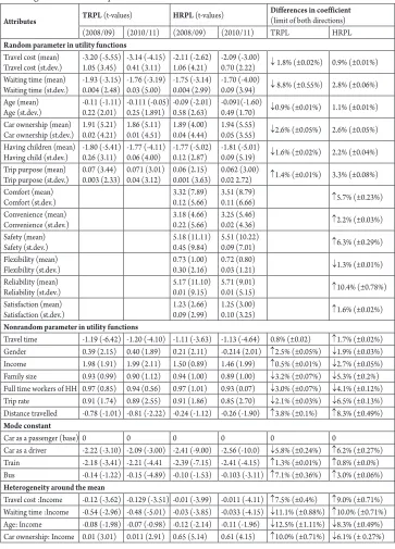
Table 4 summarises the estimated results of the two datasets with the specifications of the RPL model. A specified number of TOAs and LVs have been integrated in the models to observe the overall impacts on traveller mode choice from 2008/09 to 2010/11.

The analysis suggests that both models produce similar results when considering TOAs, but when LVs are included, the importance of LVs exceeds those of TOAs. For example, findings from both the TRPL and HRPL models suggest that in 2010/11,

travel time had a greater impact on traveller

mode choice than travel cost. Also, the effect

of trip purpose on mode choice was shown to increase between 2008/09 and 2010/11, while

the effects of family size, full time workers, and

trip rate declined. An interesting outcome was

the identified decrease in the effect of waiting

time on mode choice in both models. This

finding is consistent with those of the BTS Report (2012), which suggests the growing uptake of public transport by travellers who appear to place less importance on waiting time. Unlike the TRPL model, however, the HRPL model identified age as a significant factor in mode choice, particularly in the case of elderly people, who generally seek a comfortable or convenient mode of transport.

Similarly, the effect of car ownership is higher

in the HRPL model which indicates that a car maximises the desired utility that may come from LVs rather than TOAs.

The importance of LVs to travellers is clearly observed in the HRPL models. All of them are also statistically significant except the

variable flexibility. The variables with the

highest impact in both years were safety and

reliability, followed by comfort and convenience. Overall, the impact of LVs on mode choice was shown to increase between 2008/09 and 2010/11.

The probability of train usage was shown to increase by 2.3% and 2.1% from 2008/09 to 2010/11 according to TRPL and HRPL models respectively. On the other hand, the probability of car usage decreased by 1.1% and 1.5% in TRPL and HRPL model respectively. Bus usage increased by 2% and 1.8% accordingly. The overall differences in results between 2008/09 and 2010/11 are minimal, which suggest that changes in traveller behaviour are gradual.

Table 2

MIMIC Model Results Using 2008/09 HTS Data: α Vector Matrix of Structural Equations (t-values in the Parenthesis)

LVs Travel _time Travel _cost Waiting _time Age Income Family _size Gender Car _ownership No. _child Full _time Trip _rate Distance _travelledTrip _purpose

Comfort -0.055_(-2.10) -0.202_(-5.77) -0.175_(-2.00) -0.014_(-11.1) 0.145_(2.72) -0.008_(-3.15) 0.054_(3.35) 0.221_(5.00) 0.221_(4.21) 0.008_(2.03) 0.058_(4.68) 0.111_(4.84) 0.063_(1.75)

Convenience -0.127_(-9.51) -0.058_(-2.00) -0.222_(-4.35) -0.132_(-2.45) 0.189_(2.33) -0.006_{(-3.45) (2.85)}0.189 0.132_(5.63) 0.136_(2.89) 0.071_(3.44) 0.137_(3.43) 0.115_(2.05) 0.171_(2.00)

Flexibility -0.171_(-7.52) -0.004_(-1.99) -0.067_(2.99) -0.184_(-4.12) 0.082_(-3.50) 0.021_(5.10) -0.106_(-3.13) -0.011_(-2.50) -0.121_(-6.37) -0.037_(-3.63) 0.012_(2.00) 0.160_(8.00) 0.126_(10.5)

Safety -0.166_(-6.23) -0.100_(-3.04) -0.089_(-1.97) -0.258_(-3.45) -0.136_(-4.49) 0.011_(6.0) -0.08_(-6.85) -0.087_(-6.78) -0.121_(-6.37) -0.037_(-3.44) 0.012_(2.00) 0.168_(6.41) 0.126_(5.73)

Reliability -0.444_(-5.24) -0.022_(1.87) -0.107_(-3.33) -0.142_(-4.44) 0.026_(2.17) -0.009_(-2.10) 0.074_(3.85) 0.122_(3.21) 0.013_(4.25) 0.025_(3.13) 0.019_(3.17) 0.212_(3.45) 0.031_(2.58)

Satisfaction -0.129_(-1.98) -0.155_(-6.66) -0.077_(-2.80) -0.143_(-11.11)0.028_(4.52) -0.086_(-4.44) -0.086_(-3.45) 0.102_(6.19) 0.109_(15.25) 0.045_(5.63) 0.107_(17.83) 0.022_(7.33) 0.025_(2.08) Model fit criteria

GFI 0.927 AGFI 0.902 NFI 0.964 CFI 0.911 RMSEA Lower bound upper bound

0.043

0.030 (90% CI of RMSEA) 0.051 (90% CI of RMSEA)

Source: Anwar et al. (2014)

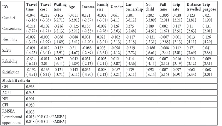
Table 3

MIMIC Model Results Using 2010/11 HTS Data: α Vector Matrix of Structural Equations (t-values in the Parenthesis)

LVs Travel _time Travel _cost Waiting _time Age Income Family _size Gender Car _ownership No. _child Full _time Trip _rate Distance _travelledTrip _purpose

Comfort -0.045_(-3.16) -0.212_(-3.86) -0.165_(-5.71) -0.011_(-2.91) 0.121_(-2.87) -0.002_(-3.01) 0.061_(-4.1) 0.301_(-6.12) 0.202_(-3.89) 0..006_(2.01) 0.038_(2.21) 0.123_(3.81) 0.021_(1.90)

Convenience -0.211_(-7.27) -0.102_(-1.71) -0.216_(-5.13) -0..125_(-2.21) 0.156_(-2.53) -0.002_{(-2.76) (-2.63)}0.126 0.275_(-5.48) 0.189_(-4.51) 0.002_(1.67) 0.117_(2.51) 0.11_(2.63) 0.131_(2.01)

Flexibility -0.092_(-3.47) -0.003_(-1.99) -0.066_(-1.89) -0.088_(-3.41) 0.031_(-1.90) 0.022_(-3.01) -0.102_(-2.13) -0.117_(-5.15) -0.131_(-5.31) -0.007_(-2.85) 0.001_(2.13) 0.013_(4.11) 0.126_(4.20)

Safety -0.091_(-4.22) -0.012_(-3.04) -0.132_(-3.91) -0.21_(-4.67) -0.088_(-2.89) 0.005_(-3.64) -0.098_(-4.12) -0.219_(-7.72) -0.166_(-6.61) -0.008_(-2.44) 0.112_(3.01) 0.171_(3.69) 0.041_(2.58)

Reliability -0.514_(-6.21) -0.011_-2.01 -0.107_(-6.11) -0.042_(-1.89) 0.031_(-2.12) -0.005_(-2.11) 0.012_(-3.07) 0.414_(-4.56) 0.003_(-4.11) 0.007_(2.12) 0.016_(3.19) 0.112_(3.12) 0.009_(2.51)

Satisfaction -0.192_(-3.91) -0.166_(-6.21) -0.121_(-3.71) -0.142_(-5.11) 0.032_(-3.90) -0.008_(-2.12) -0.087_(-3.21) 0.139_(-5.11) 0.092_(-6.15) 0.007_(5.16) 0.097_(6.91) 0.062_(5.33) 0.068_(3.01) Model fit criteria

GFI 0.963 AGFI 0.945 NFI 0.901 CFI 0.950 RMSEA Lower bound upper bound

0.033

Table 4

Modelling Results with Comparison between Two Datasets

Attributes TRPL (t-values) HRPL (t-values)

Differences in coefficient (limit of both directions) (2008/09) (2010/11) (2008/09) (2010/11) TRPL HRPL Random parameter in utility functions

Travel cost (mean)

Travel cost (st.dev.) -3.20 (-5.55)1.05 (3.45) -3.14 (-4.15)0.41 (3.11) -2.11 (-2.62)1.06 (4.21) -2.09 (-3.00)0.70 (2.22) ↓ 1.8% (±0.02%) 0.9% (±0.01%) Waiting time (mean)

Waiting time (st.dev.) -1.93 (-3.15)0.004 (2.48) -1.76 (-3.19)0.03 (5.00) -1.75 (-3.14)0.004 (2.99) -1.70 (-4.00)0.09 (3.94) ↓ 8.8% (±0.55%) 2.8% (±0.06%) Age (mean)

Age (st.dev.) -0.11 (-1.11)0.22 (2.01) -0.111 (-0.05)0.25 (1.891) -0.09 (-2.01)0.58 (2.63) -0.091(-1.60)0.49 (1.70) ↓0.9% (±0.01%) 1.1% (±0.01%) Car ownership (mean)

Car ownership (st.dev.) 1.91 (5.21)0.02 (4.21) 1.86 (5.11)0.01 (4.51) 1.89 (4.00)0.04 (4.44) 1.94 (5.55)0.05 (3.55) ↓2.6% (±0.05%) 2.6% (±0.05%) Having children (mean)

Having child (st.dev.) -1.80 (-5.41)0.26 (3.11) -1.77 (-4.11)0.06 (4.00) -1.77 (-5.02)0.12 (2.87) -1.81 (-5.01)0.09 (5.19) ↓1.6% (±0.02%) 2.2% (±0.04%) Trip purpose (mean)

Trip purpose (st.dev.) 0.07 (3.44) 0.003 (2.33) 0.071 (3.01) 0.04 (3.12) 0.06 (2.15)0.001 (3.63) 0.062 (3.00)0.02 2.72) ↑1.4% (±0.01%) 3.3% (±0.08%) Comfort (mean)

Comfort (st.dev.) 3.32 (7.89)0.12 (5.66) 3.51 (8.79)0.11 (6.66) ↑5.7% (±0.23%) Convenience (mean)

Convenience (st.dev.) 3.18 (4.66)0.22 (5.66) 3.25 (5.46)0.02 (4.36) ↑2.2% (±0.03%) Safety (mean)

Safety (st.dev.) 5.18 (11.11)0.45 (9.84) 5.51 (10.22)0.09 (7.01) ↑6.3% (±0.29%) Flexibility (mean)

Flexibility (st.dev.) 0.73 (1.00)0.30 (2.16) 0.72 (0.80)0.03 (1.21) ↓1.3% (±0.01%) Reliability (mean)

Reliability (st.dev.) 5.17 (11.10)0.01 (9.15) 5.71 (9.01)0.01 (5.15) ↑10.4% (±0.78%) Satisfaction (mean)

Satisfaction (st.dev.) 1.23 (2.66)0.09 (2.99) 1.25 (3.00)0.10 (3.25) ↑1.6% (±0.02%) Nonrandom parameter in utility functions

Travel time -1.19 (-6.42) -1.20 (-4.10) -1.11 (-3.63) -1.13 (-4.64) 0.8% (±0.02) ↑1.7% (±0.02%) Gender 0.39 (2.15) 0.40 (1.89) 0.21 (2.11) -0.214 (2.01) ↑2.5% (±0.05%) ↓1.9% (±0.03%) Income 1.98 (1.91) 1.99 (2.11) 1.50 (0.89) 1.46 (1.99) ↑0.5% (±0.01%) ↓2.7% (±0.05%) Family size 0.93 (0.99) 0.90 (1.12) 0.94 (1.00) 0.89 (1.00) ↓3.2% (±0.07%) ↓5.3% (±0.2%) Full time workers of HH 0.97 (0.85) 0.94 (0.56) 0.97 (1.01) 0.93 (0.07) ↓3.0% (±0.07%) ↓4.1% (±0.12%) Trip rate 0.91 (1.74) 0.89 (2.55) 0.91 (1.86) 0.85 (2.70) ↓2.1% (±0.03%) ↓6.5% (±0.13%) Distance travelled -0.78 (-1.01) -0.81 (-2.22) -0.24 (-1.12) -0.26 (-1.90) ↑3.8% (±0.1%) ↑8.3% (±0.49%) Mode constant

Car as a passenger (base) 0 0 0 0 0 0

Car as a driver -2.22 (-3.10) -2.09 (-3.00) -2.41 (-9.00) -2.56 (-10.0) ↓5.8% (±0.24%) ↑6.2% (±0.27%) Train -2.18 (-3.41) -2.21 (-4.41 -2.39 (-7.15) -2.41 (-4.15) ↑1.3% (±0.01%) ↑0.8% (±0.0%) Bus -0.14 (-1.22) -0.15 (-4.89) -0.10 (-1.53) -0.103 (-3.11) ↑7.1% (±0.36%) ↑3.0% (±0.06%) Heterogeneity around the mean

Attributes TRPL (t-values) HRPL (t-values) Differences in coefficient(limit of both directions) (2008/09) (2010/11) (2008/09) (2010/11) TRPL HRPL Having child: income -0.09 (-2.66) -0.1 (-3.16) -0.17 (-3.01) -0.19 (-4.07) ↑11.1% (±0.88%) ↑11.7% (±0.99%) Purpose: Income 0.01 (4.01) 0.001 (3.01) 0.05 (3.01) 0.052 (3.11) ↓9.0% (±2.01%) ↑4.0% (±0.11%) Comfort: Income 0.09 (3.10) 0.101 (4.21) ↑12.2% (±1.06%) Convenience: Income 0.10 (2.89) 0.112 (3.80) ↑12.0% (±1.03%) Safety: Income 0.45 (11.52) 0.51 (10.51) ↑13.3% (±1.27%) Flexibility: Income 0.05 (2.45) 0.052 (1.80) ↑4.0% (±0.11%) Reliability: Income 0.31 (10.20) 0.35 (9.10) ↑12.8% (±1.19%) Satisfaction: Income 0.08 (5.10) 0.089 (4.11) ↑11.2% (±0.90%) Model statistics

Log likelihood function -715.28 -696.80 -613.37 -576.53 ↓2.58% (±0.05%) ↓6.00% (±0.26%) McFadden Pseudo

R-squared 0.27 0.28 0.36 0.38 ↑3.7% (±0.1%) ↑5.56% (±0.22%) Akaike Information

Criterion (AIC) 0.0170 0.0165 0.0145 0.0136 ↓2.94% (±0.06%) ↓6.21% (±0.27%) Modal choice probability

Car as a driver 0.731 0.720 0.785 0.770 1.1% (±0.02%) ↓1.5% (±0.03%) Car as a passenger 0.055 0.049 0.010 0.020 ↓0.6% (±0.85%) ↑1.0% (±02.01%) Train 0.181 0.204 0.190 0.211 2.3% (±1.15%) ↑2.1% (±0.87%) Bus 0.033 0.053 0.015 0.033 ↑2.0% (±2.02) ↑1.8% (±2.12%)

Legend:

↑ _{means increase;} ↓ _{means decrease;}

5. Forecasting Changes in Traveller Mode

Choice

Forecasting and policy evaluation have not been discussed in the last decade to the same extent as the estimation of hybrid discrete choice models. Although the concept of LVM has been used to explore the effect of latent factors on the decision making process either through factor analysis or logistic regression, this has been done without reference to policy intervention (Mokhtarian, 1998; Cao et al., 2009; Fujii and Garling, 2003).

According to the specifications of the MIMIC model, change in the explanatory variables should cause changes in the LVs and then, these changes may have an impact on the MIMIC model as well as on the utility

functions in the choice model. Due to the changes in utility function, traveller mode choice probabilities are affected accordingly. The changes in the choice forecasting probabilities may be caused by the variations in explanatory variables related to objective attributes. The changes in the explanatory

variables sijr and the tangible attributes Xijk

may affect the choices implicitly through the LVs or the alternative utilities respectively by which the changes in choice probabilities may be observed.

LVs impact on mode choice to influence overall trips structure. Thus, the transport forecasting context is an interrelationship among various observed and unobserved factors related transport management system and it is understood that traditional mode choice models (without LVs) are not generally sensitive to policies which affect the transport management system. Policies are associated with the changes over the management system which, in turn, may have an impact on the observed mobility structure of the travellers. Thus, the LVs would be able to capture transport system changes because the explanatory variables are related to demographics as well as the alternatives included in the MIMIC model to evaluate the

traveller motivational process. The way what authors described is an important measure to be considered for forecasting the changes using the estimated models.

On the basis of the empirical case presented in this paper, we tested three hypothetical scenarios of (i) increasing individual income with 10%; (ii) reducing travel cost and waiting time for public transport with 10%; and (iii) implementing both (i) and (ii) concurrently to compare the forecasting performance of the estimated models. The variation of income affects directly: (i) the LV, as income is an explanatory variable in the MIMIC model and (ii) the utility functions, due to inclusion of it in the utility functions.

Table 5

Forecasting Changes in Traveller Mode Choice

Mode Base year market share in %

Predicted changes♦

Scenario 1 (S1) Scenario 2 (S2) Scenario 3 (S3)

TRPL HRPL TRPL HRPL TRPL HRPL TRPL HRPL

Car as a driver 73.1 78.5 -0.07 0.21 -1.00 -0.85 -0.54 -0.32 Car as a passenger 5.5 1.0 -0.04 0.08 -0.08 -0.01 -0.06 0.04

Train 18.1 19.0 0.33 0.17 0.95 0.52 0.64 0.35

Bus 3.3 1.5 -0.08 -0.04 0.51 0.48 0.22 0.22

S1: Individual income is increased with 10%

S2: Travel cost and waiting time for public transport are reduced with 10% S3: S1 and S2 are implemented concurrently

♦ Changes, that were calculated using 2010/11 HTS data only, are the differences of the

probabilities between changed and unchanged condition.

Table 5 presents the base year market shares which are estimated by each model under no-change conditions. The market share changes are predicted by the estimated models with three hypothetical scenarios. Due to the complexity of the probability function (Eq. (10)), it is difficult to get exact resolution of the choice probabilities but a reasonable idea can be obtained about the forecasting from these iterations.

by train which is an interesting finding to help policy makers.

As per S2, the probabilities of train and bus use are increased for both TRPL and HRPL models; it implies that reduction of travel cost and waiting time are helpful to reduce the travel by car. Furthermore, it is observed that the predicted changes of train and bus usage probability are the highest in TRPL model of S2 compared with other scenarios. This implies that the reduction of travel time and waiting time are most likely to increase public transport usage. In S3, TRPL model shows that probabilities of car use as a driver and a passenger are reduced while the condition of S1 and S2 are implemented concurrently. On the other hand, probability of train usage is higher than HRPL model as increasing individual income and reduced travel cost and waiting time are included together.

Additionally, as expected, HRPL model in S1 predicts an increase in private modes due to increasing income as a changed condition, while the other HRPL models in S2 and S3 forecast a decrease in private modes because of inclusion of reduced travel cost and waiting time as a changed condition. This may indicate that the hybrid RPL models are effectively more sensitive, as we expected, but this higher sensitivity does not imply just a simple amplification of the effects involved. Consequently, it is even more clear the importance of including LV in the choice models.

6. Discussions

According to the analysis of HRPL models, it could be concluded that the hybrid model is clearly superior in terms of goodness of fit over TRPL models that do not incorporate

LV and it shows the travellers’ insight motivational behaviour.

Both TRPL and HRPL models, estimated with real data collected from SSD, reveals that LVs have significant effects over the choice process. Moreover, the influences of LVs on utility functions vary significantly among individuals. The introduction of LVs in RPL models allows us not only to improve model fit, but also to achieve better estimated parameter.

The inclusion of LVs in RPL model has improved the ability of the RPL model to explain the travellers’ behaviour. On the other hand, the exclusion of LVs from the choice models is not policy sensitive as there is a big gap between the behaviour considering with and without human psychological factors (i.e. LVs). Thus, certain policies may influence particular individual’s behaviour and therefore, it could be strongly recommended to pay appropriate attention to LVs.

safety value is increased and thereby also the relevance of security for mode choice becomes important. Moreover, the results support the contention that travellers’ preference heterogeneity is an important determinant in the process of mode choice. The general theoretical conclusion of this study is that future projects can be successful by including LVs of travellers.

7. Conclusions, Contributions and

Implications

The contribution of this research is

three-fold: firstly, it models the LVs and TOAs

separately and concurrently to evaluate the impact of traveller choice on mode;

secondly, it illustrates the superiority of the hybrid RPL model over the traditional RPL model along with the changes of impact on mode choice from 2008/09 to 2010/11; and

finally, it demonstrates the predicted changes (i.e. forecasting) of traveller mode choice considering hypothetical scenarios.

Besides, t h is resea rch ma kes some methodical and theoretical contributions. Concerning the methodical contribution, this research has been extended in two major ways: (i) forecasting and comparing traveller choice behaviour temporally considering TOAs and LVs; and (ii) analysing the importance/merits of LVs over objective attributes between TRPL and HRPL models towards mode choice. The HRPL model clearly outperforms a TRPL model on several counts and provides valuable insights into the motivational process that determine mode choice. A further contribution of this paper is that it suggests and demonstrates a convenient alternative for estimating HRPL model with a structural equation modelling (SEM). From a substantial point of view, HRPL model can be considered as one of

the most interesting advances in discrete choice modelling in the last decade.

With respect to the theoretical contribution, we set out to develop a more comprehensive model of choice that also maps the impact of such abstract motivational constructs as values on travellers’ real choices. The general structure of our HRPL model consists of a discrete choice part where LVs enter as explanatory variables in addition to the observed attributes of the different choice options as well as attributes of the decision maker. The latent variable part of the model allows for relations between the LVs and TOAs, as well as the contribution of LVs to traveller mode choice. Additionally, socio-economics are included as explanatory variables both in the discrete choice and the latent variable model in order to control for observed heterogeneity and to aid in forecasting the latent variables. In our empirical example, the HRPL model where personal characteristics determine latent preferences which in turn impact on actual behaviour, was proposed and validated.

The policy response should consider travellers’ expectations to solve the problem. Although it has been recognised as important by transport analyst, it has not been adequately reflected in the current policy responses since the probability of using a private car is dominantly high. Therefore, this study has clarified the nature of traveller preference heterogeneity both observed and unobserved in the process of mode choice showing a hierarchy of importance, which could assist in formulating effective and fruitful policies.

Acknowledgments

The authors are grateful to the personnel of Bureau of Transport Statistics (BTS) affiliated with Transport for NSW, Australia for providing access to the largest and most comprehensive household travel survey data of SSD. The University of Wollongong, especially SMART Infrastructure Facility, also deserves special thanks for financial support to carry out this research.

References

Anwar, A.H.M.M.; Tieu, K.; Gibson, P.; Win, K.T.; Berryman, J.M. 2014. Analysing the heterogeneity of traveller mode choice preference using a random parameter logit model from the perspective of principal-agent theory, International Journal of Logistics Systems and Management. DOI: http://dx.doi.org/10.1504/ IJLSM.2014.061015, 17(4): 447-471.

Anwar, A.H.M.M.; Tieu, K.; Gibson, P.; Win, K.T.; Berryman, J.M. 2013. Analysing the merit of latent variables over traditional objective attributes for traveller mode choice using RPL model. In Proceedings of the 3rd _{International Choice Modelling Conference, online,}

Sydney.

A nw a r, A . H . M . M .; Tieu, K .; Gibson, P.; Berryman, J.M.; Win, K.T. 2011. Structuring the influence of latent variables in traveller preference heterogeneity. In Transportdynamics – Proceedings of the 16th _{International Conference of Hong Kong Society} for Transportation Studies, (ed. W.Y. Szeto, S.C. Wong and N.N. Sze): 141-148.

Ashok, K.; William, R.D.; Yuan, S. 2002. Extending discrete choice models to incorporate attitudinal and other latent variables, Journal of Marketing Research. DOI: http://dx.doi.org/10.1509/jmkr.39.1.31.18937, 39(1): 31-46.

Ben-Akiva, M.; McFadden, D.; Train, K.; Walker, J.; Bhat, C.; Bierlaire, M.; Bolduc, D.; Boersch-Supan, A.; Brownstone, D.; Bunch, D.S.; Daly, A.; Palma, A.D.; Gopinath, D.; Karlstrom, A.; Munizaga, M.A. 2002a. Hybrid choice models: progress and challenges, Marketing Letters. DOI: http://dx.doi. org/10.1023/A:1020254301302, 13(3): 163-175.

Ben-Akiva, M.; Walker, J.L.; Bernardino, A.T.; Gopinath, D.A.; Morikawa, T.; Polydoropoulou, A. 2002b. Integration of choice and latent variable models. In Perpetual motion: travel behaviour research opportunities and challenges, (ed. HS Mahmassani), Amsterdam Pergamon: 431-470.

Ben-Akiva, M.; Bradley, M.; Morikawa, T.; Benjamin, J.; Novak, T.; Oppewal, H.; Rao, V. 1994. Combining revealed and stated preferences data, Marketing Letters. DOI: http://dx.doi.org/10.1007/BF00999209, 5(4): 335-350.

Bhat, C.R. 2000. Incorporating observed and unobserved heterogeneity in urban work travel mode choice modelling, Transportation Science. DOI: http://dx.doi. org/10.1287/trsc.34.2.228.12306, 34(2): 228-238.

Bolduc, D.A. 1999. Practical technique to estimate multinomial probit models in transportation,

Transportation Research Part B: Methodological. DOI: http://dx.doi.org/10.1016/S0191-2615(98)00028-9, 33(1): 63-79.

Bolduc, D.; Boucher, N.; Alvarez-Daziano, R. 2008. Hybrid choice modelling of new technologies for car choice in Canada, Transportation Research Record: Journal of the Transportation Research Board. DOI: http://dx.doi. org/10.3141/2082-08, 2082(2008): 63-71.

Bureau of Transport Statistics (BTS). 2012. 2010/11 Household travel survey summary report, 2012 release, Transport for New South Wales, Sydney.

Byrne, B.M. 2010. Structural equation modelling with AMOS: Basic concepts, applications, and programming, 2nd _{ed., New}

York, Routledge.

Can, V.V. 2013. Estimation of travel mode choice for domestic tourists to Nha Trang using multinomial probit model, Transportation Research Part A: Policy and Practice. DOI: http://dx.doi.org/10.1016/j.tra.2013.01.025, 49: 149-159.

Cao, X.; Mokhtarian, P.L.; Handy, S.L. 2009. Examining the impacts of residential self-selection on travel behaviour: A focus on empirical findings, Transport Reviews: A Transnational Transdisciplinary Journal. DOI: http://dx.doi.org/10.1080/01441640802539195, 29(3): 359-395.

Choo, S.; Mokhtarian, P.L. 2004. What types of vehicle do people drive.? The role of attitude and lifestyle in influencing vehicle type choice, Transportation Research Part A: Policy and Practice. DOI: http://dx.doi. org/10.1016/j.tra.2003.10.005,38(3): 201-222.

Cohen, A.; Harris, N. 1998. Mode choice for VFR journeys, Journal of Transport Geography. DOI: http:// dx.doi.org/10.1016/S0966-6923(97)00038-0, 6(1): 43-51.

Commins, N.; Nolan, A. 2011. The determinants of mode of transport to work in the greater Dublin area,

Transport Policy. DOI: http://dx.doi.org/10.1016/j. tranpol.2010.08.009, 18(1): 259-268.

Daly, A.; Hess, A.; Patruni, B.; Potoglou, D.; Rohr, C. 2012. Using ordered attitudinal indicators in a latent variable choice model: A study of the impact of security on rail travel behaviour, Transportation. DOI: http:// dx.doi.org/10.1007/s11116-011-9351-z, 39(2): 267-297.

Dissanayake, D.; Morikawa, T. 2005. Household travel behaviour in developing countries: Nested logit model of vehicle ownership, mode choice, and trip chaining,

Transportation Research Record: Journal of the Transportation Research Board. DOI: http://dx.doi.org/10.3141/1805-06, 1805(2002): 45-52.

Domarchi, C.; Tudela, A.; Gonzalez, A. 2008. Effect of attitudes, habit and affective appraisal on mode choice: An application to university workers, Transportation. DOI: http://dx.doi.org/10.1007/s11116-008-9168-6, 35(5): 585-599.

Ewing, R.; Schroeer, W.; Greene, W. 2004. School location and student travel analysis of factors affecting mode choice, Transportation Research Record: Journal of the Transportation Research Board, 1895: 55-63.

Fesenmaier, D.R. 1988. Integrating activity patterns into destination choice models, Journal of Leisure Research, 20(3): 175-191.

Fujii, S.; Garling, T. 2003. Application of attitude theory for improved predictive accuracy of stated preference methods in travel demand analysis, Transportation Research Part A: Policy and Practice. DOI: http://dx.doi. org/10.1016/S0965-8564(02)00032-0, 37(4): 389-402.

Gopinath, A.D. 1995. Modeling heterogeneity in discrete choice processes: application travel demand, PhD thesis, Massachusetts Institute of Technology, USA.

Greene, W.H.; Hensher, D.A. 2003. A latent class model for discrete choice analysis: contrasts with mixed logit,

Transportation Research Part B: Methodological. DOI: http:// dx.doi.org/10.1016/S0191-2615(02)00046-2, 37(8): 681-698.

Habib, K.M.N. 2012. Modeling commuting mode choice jointly with work start time and work duration,

Transportation Research Part A: Policy and Practice. DOI: http://dx.doi.org/10.1016/j.tra.2011.09.012, 46(1): 33-47.

Habib, K.M.N.; Zaman, M.H. 2012. Effects of incorporating latent and attitudinal information in mode choice models, Transportation Planning and Technology. DOI: http://dx.doi.org/10.1080/03081060.2012.701 815, 35(5): 561-576.

Hess, S.; Stathopoulos, A. 2011. Linking response quality to survey engagement: A combined random scale and latent variable approach. In Proceedings of the 2nd _{International Choice Modelling Conference, Leeds, UK.}

Hess, S.; Stathopoulos, A.; Daly, A. 2011. Allowing for heterogeneous decision rules in discrete choice models: an approach and four case studies. In Proceedings of the 2nd _{International Choice Modelling Conference, Leeds, UK.}

Jialing, H.; Jun, L.; Xinjun, L.; Honggang, X. 2013. Modal choice of recreational tourists under regional transportation integration: A case study of pearl river delta, Applied Mechanics and Materials. DOI: http://dx.doi.org/10.4028/ www.scientific.net/AMM.253-255.287, 253-255: 287-292.

Johansson, M.V.; Heldt, T.; Johansson, P. 2006. The effects of attitudes and personality traits on mode choice,

Transportation Research Part A: Policy and Practice. DOI: http://dx.doi.org/10.1016/j.tra.2005.09.001, 40(6): 507-525.

McCarthy, P. 1996. Market price and income elasticities of new vehicle demands, The Review of Economics and Statistics, 78(3): 543-547.

Mokhtarian, P.L. 1998. A synthetic approach to estimating the impacts of telecommuting on travel, Urban Studies. DOI: http://d x.doi. org/10.1080/0042098984952, 35(2): 215-241.

Nicolau, J.L.; Mas, F.J. 2006. The influence of distance and prices on the choice of tourist destinations: The moderating role of motivations, Tourism Management. DOI: http://dx.doi.org/10.1016/j.tourman.2005.09.009, 27(5): 982-996.

Ortuzar, J.de D.; Willumsen, L.G. 2001. Modelling transport, 3rd _{ed. Chichester, John Wiley and Sons.}

Raveau, S.; Alvarez-Daziano, R.; Yanez, M.F.; Bolduc, D.; Ortuzar, J.de D. 2010. Sequential and simultaneous estimation of hybrid discrete choice models: Some new findings, Transportation Research Record: Journal of the Transportation Research Board. DOI: http://dx.doi. org/10.3141/2156-15, 2156(2010): 131-139.

Sheriff, K.M.M.; Gunasekaran, A.; Nachiappan, S. 2012. Reverse logistics network design: A review on strategic perspective, International Journal of Logistics Systems and Management. DOI: http://dx.doi.org/10.1504/ IJLSM.2012.047220, 12(2): 171-194.

Temme, D.; Paulssen, M.; Dannewald, T. 2008. Incorporating latent variables into discrete choice models – A simultaneous estimation approach using SEM software, BuR Business Research Journal. DOI: http:// dx.doi.org/10.1007/BF03343535, 1(2): 220-237.

Train, K. 2009. Discrete choice method with simulation, 2nd

ed. New York, Cambridge University Press.

Train, K.E. 1998. Recreation demand models with taste differences over people, Land Economics, 74(2): 230-239. Train, K.E. 1980. A structured logit model of auto ownership and mode choice, Review of Economic Studies. DOI: http://dx.doi.org/10.2307/2296997, 28(2): 357-370.

Walker, J.L.; Ben-Akiva, M. 2002. Generalized random utility models, Mathematical Social Sciences. DOI: http:// dx.doi.org/10.1016/S0165-4896(02)00023-9, 43(3): 303-343.

Washbrook, K.; Haider, W.; Jaccard, M. 2006. Estimating commuter mode choice: A discrete choice analysis of the impact of road pricing and parking charge, Transportation. DOI: http://dx.doi.org/10.1007/s11116-005-5711-x, 33(6): 621-639.